Flight Safety and Consumer Br and Choice Behavior in the Inter national Flight Categor y
By
Couchen Wu Professor
Department of Business Administration National Taiwan University of Science and Technology
43 Keelung Road Sec. 4, Taipei City, Taiwan
Flight Safety and Consumer Br and Choice Behavior in the Inter national Flight Categor y
Abstr act
In this paper we study the influence of consumer learning behavior on brand switching in the international flight category and predict consumer brand-switching and brand-loyalty behavior by using past purchasing behavior. After empirically studying two airline markets in the Asia-Pacific area, interestingly, there are substantial findings that the impact of state-dependence is quite significant over time. Even though one of the major players, China Airlines, experienced a tragic aircraft crash in Japan within the observation period, the brand-switching and brand-loyalty probabilities were still highly correlated with previous corresponding probabilities.
Keywor ds: International Airlines, State-dependence Effect, Brand Switching
1. Introduction
With an eye to future prosperity, most international airlines are considering a range of developments that extend far into the future and from which they expect to win a greater market share. In order to win this market share, it is first necessary to realize consumers’
brand choice behavior. Consumers do change their buying behavior over time. The most important factor in making such a change is called learning (Kuehn, 1962). Learning describes changes in an individual’s behavior arising from experience (Kotler and Armstrong, 1991). Grunert (1996) defines learning as:
"In a memory conceived of as a network of nodes and links, learning amounts to adding new nodes, adding new links, and/or strengthening existing links (e.g., learning about new products or product attributes, learning that a product possesses a certain attribute, or reinforcing an existing belief that a product possesses this attribute)."
Stochastic models were proposed as a framework to help understand patterns of consumers’ learning behavior and the influence of learning on brand switching. Estes (1954) and Bush and Mosteller (1955) proposed the stochastic learning model, and showed that it could describe consumers’ brand switching. According to this concept, Kuehn (1958) found evidence that consumer purchasing decisions are a learning process.
He proposed that every past purchase decision affects subsequent purchase decisions, and the more recent the purchase the greater the effect. Kuehn assumed a homogeneous population of consumers in which the current purchase decision is influenced by at least the last four or five most-recent purchase decisions.
Recent models to help understand consumer brand choices (Erdem et al. 1996, Keane 1997) adopting logit and probit models were derived from a theory of utility maximization. Within the context of random utility models, researchers have also investigated the learning effects of past choices on a consumer’s current choice, which is the so-called effect of state dependence on brand choice. In some cases, state dependence
may be positive and consumers routinize their brand purchases by buying the same brand repeatedly over time (Howard and Sheth 1969), that is, the currently chosen brand has a higher probability of being chosen in the future than other brands. On the other hand, state dependence may be negative and consumers may be “satiated” with previously chosen brands, and switch brands in a quest for variety (McAlister 1982).
Researchers have also accommodated state dependence in random utility models by scanning consumer purchase behaviors for convenience products such as detergent, ketchup, peanut butter, margarine, toilet tissue, and tuna, etc. (e.g., Guadagni et al. 1983, Erdem et al. 1996, Seetharaman et al. 1999). The general purposes of this literature are to explore the influence of state dependence on brand choice and to predict consumers’
brand-choice behaviors. The important measure of brand-choice behavior, brand-choice probability, is obtained by applying logit or probit models.
When the impact of state dependence on brand choice behavior is substantial, it can be inferred that the consumer’s brand-choice behaviors follow some patterns, and the future brand-choice behaviors should depend on current or even past brand-choice behaviors.
That is, future brand-choice probabilities depend on current or past brand-choice probabilities. However, the previous literature did not study this issue or address the possibility of future brand-switching probabilities being predicted by using current and past brand-switching probabilities. In addition, they focused on consumer product categories and not on the international flight category.
Consumer brand-choice behavior in the international flight category may be different from corresponding behavior in consumer product categories. For example, consumers may have higher expectations about flying, or they may become extremely irritated when problems arise (Nelms 1991). Therefore, the purposes of this paper are to study the influence of consumer learning behavior on brand switching in the international flight
category and to predict consumer brand-switching and brand-loyalty behaviors by using past purchasing behavior. Because applying the previous learning framework usually causes computational difficulties (Erdem et al. 1996), we thus propose a simple learning model to analyze consumers’ brand-switching behavior. Two airline markets in the Asia- Pacific area were selected for the empirical study, since more than 50% of the world’s 736 million international airline passengers will be flying to, from, or within this region by the year 2010 (Stein, 1996). Interestingly, there are substantial findings that the impact of state-dependence is quite significant over time; even when a major player, China Airlines, experienced a major tragic airplane crash in Japan within the observation period, the brand-switching and brand-loyalty probabilities were still highly correlated with previous corresponding probabilities.
2. The model
The behavior of brand switching is generally analyzed by a brand-switching and brand-loyalty table (Churchill 1999), that is to employ a first-order Markov model of discrete choice (Heckman 1981) to describe consumers’ brand-choice behaviors. In applying such a model, it is assumed that consumers’ purchase behaviors are majorly affected by experience with the most recent purchase. In studying learning behavior via brand switching, unlike a Markov chain formulation in which the time between transitions is fixed, such an analysis only counts the event of purchase. The resulting formulation is therefore a semi-Markov model that incorporates a simple framework of learning and brand switching (Ross 1983).
Brand-switching probabilities can be stationary or nonstationary. In stationary conditions, brand-switching probabilities would be the same for every transition, but under nonstationary conditions, these probabilities would differ. Let P(n), n ≥1, be the transition
matrix which involves the brand-loyalty and brand-switching probabilities within the nth purchase and the n+1st purchase. In the case of being stationary, P(n) = P(n-1) = … = P(1) for all n, n ≥1, but under nonstationary conditions, the equality does not hold.
Through learning, people acquire beliefs and attitudes which in turn affect their buying behavior and brand-choice decisions over time. We thus infer that brand-switching probabilities should be nonstationary, and that state-dependence effects should diminish as consumers become sophisticated. Also due to consumer brand-choice decisions being influenced by past experience, P(n) values should be highly correlated with each other and should show some functional relationships. Therefore, to study the existence of learning, it is necessary to examine whether transition probabilities are stationary or not. To develop a model incorporating learning and brand switching to predict future brand- switching probabilities, it is necessary to study the past purchase history and brand-choice decisions. Brand-choice decisions are affected by many factors, including brand loyalty, promotions, price discounts, and the last purchase behavior, but they are impacted significantly by the last purchase occasion (Kuehn 1962).
Once transition probabilities are nonstationary and the learning effect exists, we can hypothesize P(n+1) to be a function of P(n), P(n-1),… , and P(1). A simple learning model for
predicting future brand switching probabilities can be as:
where:
P(n) = [ pij(n)]m×m A(l) = [ aij(l)]m×m B = [ bij ]m×m
(1)
ε
+ +
= − +
=
+
∑
A P BP
(e) (n e 1)
n
1 e ) 1 n (
h j g i ij n
j m
i
W X, ,
1 1
∑ε
∑= =
ε = [ εij]m×m pij(n)
= the transition probability from brand i to brand j at the nth transition bij = adjusted constant of transition probability from brand i to brand j aij(l)
= marginal learning propensity
εij = random error terms and εij∼N(0, σ2).
In order to estimate the parameters of aij(l) and bij, we transform the matrix-type regression function into a single-equation regression function. The single-equation regression function is
where:
Xi,g =
Wj,h =
In equation (2), when Xi.g = 1, and Wj,h = 1, y(n+ 1)gh would be the transition probability from brand g to brand h of the n+1st transition. To make such a transformation, the random error term should be taken into account. In the single-equation regression function, only one error term is allowed, but in our case, there are m×m error terms, since to make the prediction more correctly, we allow each equation to have its own error term. As in equation (2), only one Xi.g and one Wj,h can be 1, the others should be 0, and every εij follows a normal distribution with a mean of 0 and
variance of σ2, therefore, still follows a normal distribution with mean of 0 and variance of σ2 (Billingsley 1991). Then, the equation can be employed to estimate the parameters of aij(l)
and bij.
1
if i=g
0 otherwise 1 if j=h 0 otherwis e
) 2 ( )
(
1 1 1 1
, , ,
,
1 1 1 1
, , ) 1 ( )
( )
1
(
∑∑∑ ∑ ∑∑ ∑∑
= = = =
= = = =
+
−
+ = + m +
j m
i
m
j m
i
h j g i ij h
j g i ij
n m
k m
i
m
j
h j g i e n kj ik
n
gh a p X W b X W X W
y ε
l
l
3. Empir ical examination
The empirical study examines two airline markets in the Asia-Pacific area: Taipei to Hong Kong and Taipei to Singapore.
3.1 Airline market from Taipei to Hong Kong
The market is shared by two major competing airlines: Cathay Pacific Airways (CX) and China Airlines (CI) as well as other airlines with much smaller shares. The scanner panel data was collected from government agencies of the Republic of China for 6 years (January 1991 to December 1996). Data show that 974 customers took the route at least twice, and 688 of them took it at least three times. Most customers selected Cathay Pacific Airways (CX) or China Airlines (CI), with a few of them taking one of the other airlines. Their average shares were 33.8%, 29.1%, and 37.1%, respectively. We divided the airlines into three categories and defined Cathay Pacific Airways (CX) as Brand 1, China Airlines (CI) as Brand 2, and the others as Brand 3.
The major marketing activity during the observation period was a promotion of accumulated mileage, for example, Cathay Pacific offered the Advanced Mileage Program. However, a major event that impacted consumer brand choice behavior was the tragic crash of an A300-600R of China Airlines at Nagoya, Japan in 1994. In this tragic crash, all 264 passengers and crew were killed, and the airline’s safety record was called into question. Despite this, we still proceeded with our examination of the correlation of brand-switching probabilities and verification of the effectiveness of our proposed models.
In this market, all airlines who own the right of navigation have signed a contract authorized by both the Taiwanese and Hong Kong governments, that limits the number of flights of each airline; in addition, no new competitors are allowed. To reduce the
capacity constraint effect, since it may prevent consumers from having a choice in taking an airline, we examined the loading rate. The average loading rate was under 70%.
Except during the Chinese New Year holiday, at all other times, vacancies were available.
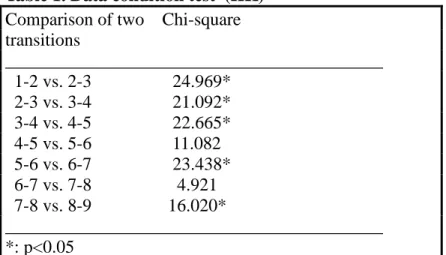
We first tested whether brand switching in this market is stationary or nonstationary, using the Chi-square test to examine the difference of these transition matrices, P(n)s. The result indicates that it is nonstationary because the observed results show significant differences (Table 1). In this case, we conclude that the traditional brand transition does not hold. As the brand-transition probabilities are not stationary and keep changing over time, we would like to understand the patterns of brand transition with the help of a learning model.
3.1.1 Goodness-of-fit of learning model
According to our hypothesis, P(n+1) is a function of P(n), P(n-1),… , and P(1). To simplify our verification, we begin with a simple learning model:
P(n+1) = A P(n) + B + ε.
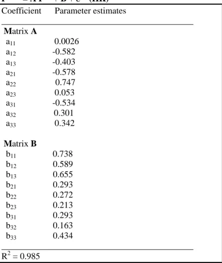
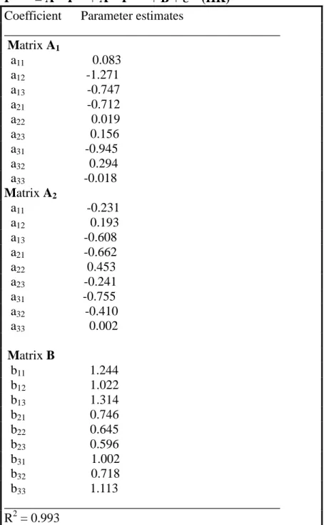
To apply such a model, there are eighteen parameters to be estimated. The parameters are estimated by a regression function; this regression equation has significant power of prediction with high R-squared values (R2 = 0.985). Table 2 displays the results for the least-squares estimation of the regression model. The simple linear learning regression model already provides good prediction power with a high R-squared value. In order to examine the significance of the influence of the second-order brand choice probabilities, i.e., the influence of P(n-1) on P(n+1), we proceeded to verify the following model P(n+1) = A(1) P(n) + A(2) P(n-1) + B + ε. Interestingly, R squared is 0.993. Such a difference is not quite significant. Therefore, in this case, we propose that the first-order linear model provides sufficient predictive power for evaluating the transition matrix of every
repurchase.
3.1.2 Comparison of learning and stationary models
In order to determine the effectiveness of the learning model and to make it more convincing, we compared the prediction results of the learning model and the results of the stationary model based on the panel data. Such a result can be used to predict future purchase behavior. The prediction result will affect market share forecasting.
In the stationary model, the transition probabilities are the same for every transition.
We also used learning model to calculate the respective predictive transition frequencies.
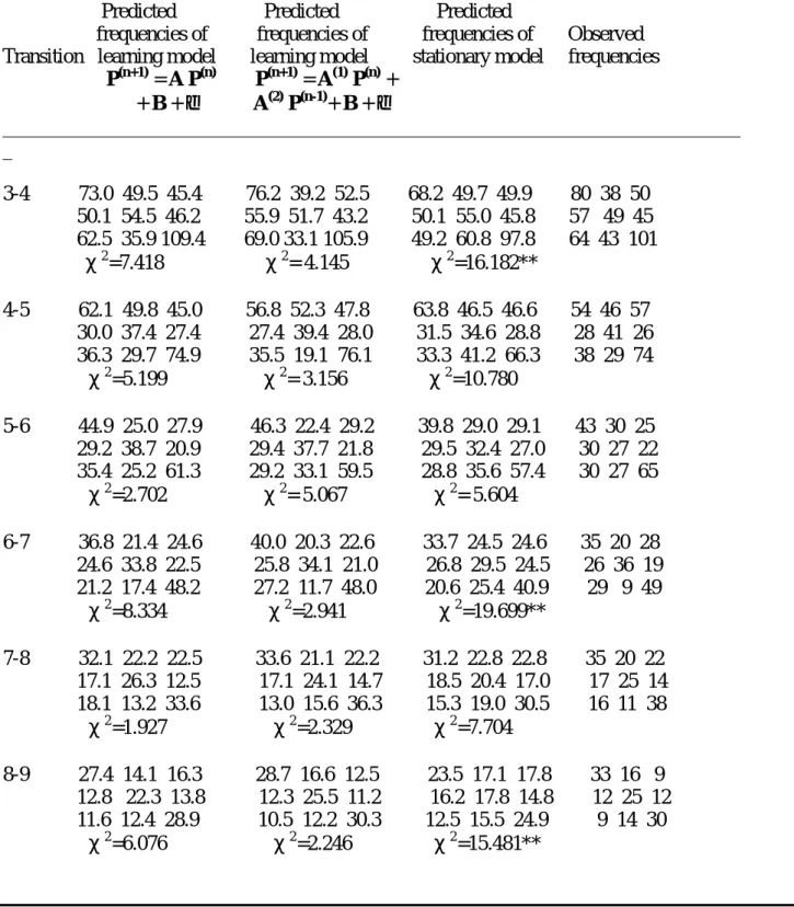
The process was performed consecutively from the second to the ninth transition. We thus compared both transition frequencies with the observed frequencies, and tested their goodness-of-fit by Chi-square test (see Table 4).
The results indicate that the learning model has more effective predictive power than does the stationary model. The transition frequencies obtained from the linear learning model have no significant difference with observed frequencies. Also, its predictive probabilities are very close to the observed probabilities which produce a diagonal result gradually. However, there are predicted frequencies by the stationary model that are significantly different from the observed frequencies.
3.2 The airline market from Taipei to Singapore
Many airlines offer flights in this market, including United Airlines, Singapore Airlines, China Airlines, and Eva Airlines. During the observation period, the airlines with the prominent market share were China Airlines and Eva Airlines. We thus separate the market into three brands: the first being China Airlines, the second being Eva Airlines, and the third being an aggregation of the other airlines. The scanner panel data was also
collected from a government agency of the Republic of China for 6 years (January 1991 to December 1996). The data show that 1050 customers took the route at least twice, and 849 of them took it at least three times. Most customers selected China Airlines (CI) or Eva Airlines (EV), with some taking one of the other airlines. Their average shares were 23.5%, 16.3%, and 60.2%, respectively.
The major marketing activity during the observation period was also the promotion of accumulated mileage such as Eva Airlines’ “Evergreen Club”. There also is a government contract restricting the number of flights of each airline and the entrance of any new competitors. To reduce the capacity constraint, since it may influence consumers’ choice behavior in selecting the airline, we examined the loading rate. The average loading rate is about 70% and vacancies are almost always available.
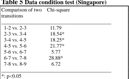
We proceeded with the same approaches as we did in the Taiwan-to-Hong Kong market. The result of stationary examination of transition matrices indicates that they are nonstationary (Table 5). We then further examined the goodness-of-fit of learning model.
3.2 Goodness-of-fit learning model
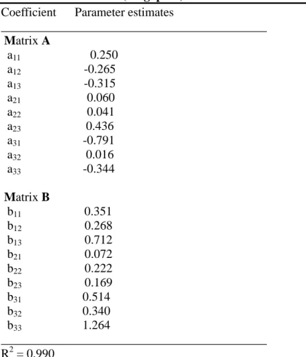
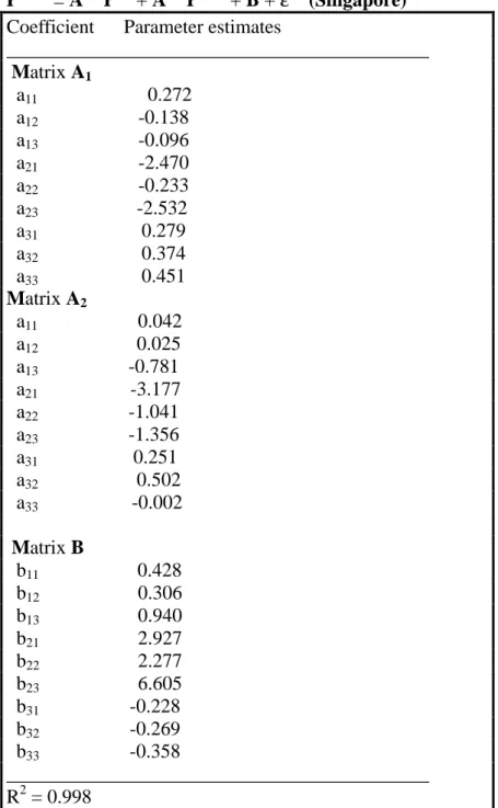
We still begin with a simple learning model, that is P(n+1) = A P(n) + B + ε. Table 6 displays the results for the least squares estimation of the regression model and shows that the simple linear learning regression model provides good predictive power with high R- squared. However, we still need to examine the significance of the influence of second- order brand choice probabilities, that is, the influence of P(n-1) on P(n+1) and proceed to verify the following model P(n+1) = A(1) P(n) + A(2) P(n-1) + B + ε. Interestingly, the difference of R squared is not significant (Table 7). Therefore, in this case, we propose that the first-order linear model provides sufficient predictive power for evaluating the transition matrix of every repurchase. By comparison with the stationary model, the
predicting result indicates that the learning model has more effective predictive power, as shown in table 8.
4. Substantial findings and manager ial implications
After examining the two airlines, we have the following substantial findings. The first interesting finding is that, even if there is a significant event impacting consumer choice behavior, i.e., a tragic aircraft crash, future brand transition probabilities are still highly correlated with current or past corresponding probabilities. In other words, future brand- switching probabilities can be predicted well by current and past brand-switching probabilities. Instead of using traditional logit or probit models, we can predict customers’ choice behavior by observing their past choice behavior. The second interesting finding is that the state-dependence effect always exists in our product categories. Seetharaman et al. (1999) reviewed the state-dependence effects over time for five consumer product categories: ketchup, peanut butter, stick margarine, toilet tissue, and canned tuna. They concluded that the state-dependence effect wears out when households become sophisticated. However, it does not occur in our product category, air transportation. The state-dependence effect is quite significant. Subsequent brand choice is highly dependent on current choice. This may be due to airlines’ accumulated mileage promotion programs, or because when selecting air transportation, consumers are more highly involved than with general consumer products. The final finding is the significance of the learning effect when selecting airlines. Brand-switching and brand-loyalty probabilities change over time. As long as a customer gets experience, the brand- transition probability will differ.
These findings have important managerial implications. For example, due to the significance of state-dependence, consumers are more inertial, and marketing program performance should focus on consumer relationship building. Rather than creating only
short-term sales for temporary brand switching, the performance of marketing variables should help to reinforce the product’s position in the market and retain customers. This is why most airlines not only promote the advantages of accumulated mileage but also provide other travel packages such as discounts for car rentals or hotel lodging. Another important managerial implication is to address the importance of initial brand choice. A marketing manager should promote the airline by making the airline the new customers’
brand choice set. Once consumers board an airline once, they have a higher probability of choosing this airline in the future. Finally marketing managers should review the customer base from time to time to observe their purchasing behavior, since brand choice behavior is highly dependent on past behavior. This type of review would be very helpful in setting up powerful marketing programs.
5. Conclusions and future research directions
The results of our study support two broad assertions. First, the learning effect is significant in brand choice of airlines. Due to learning, the transition among competitive brands is nonstationary. The stationary assumption of the Markov process of brand switching is impractical. Second, we have determined that a simple learning model is helpful in understanding patterns of brand choice and predicting brand-switching and brand-loyalty probabilities. Through use of a model, marketing manages can predict transition probabilities and market share more accurately.
Future research can extend this model by considering the following issues: 1. Are individuals that are relatively more state-dependent in the airline category also relatively more inertial in other product categories? 2. Do individuals' state dependence decrease as the time until their next purchase increases? 3. What is the relationship between individuals' sensitivity to marketing variables (price, service, etc.) and their level of state
dependence?
Reference
Billingsley, Patrick (1991), Probability and Measure, New York: Wiley.
Bush, Robert R. and Mosteller, Frederick (1955), Stochastic Models for Learning, New York: John Wiley.
Churchill, Gilbert (1999), Marketing Research: Methodological Foundations, 7th ed., Orlando, FL: The Dryden Press.
Erdem, T. and M. Keane (1996), “Decision-making Under Uncertainty: Capturing Dynamic Brand Choice Processes in Turbulent Consumer Goods Markets”, Marketing Science 15, 1, 1-20.
Estes, William K. (1954), “Individual Behavior in Uncertain Situations: An Interpretation in Terms of Statistical Association Theory,” In Thrall, R. M., C. H. Coombs, and R. L.
Davis (Eds.), Decision Processes. New York: John Wiley.
Grunert, Klaus G. (1996), “Automatic and Strategic Processes in Advertising Effects,”
Journal of Marketing, Vol. 60, October, pp.88-101.
Guadagni, Peter M. and Little, John D. C. (1983), “A Logit Model of Brand Choice Calibrated on Scanner Data,” Marketing Science, Vol.2, Summer, pp.203-238.
Heckman, J. J. (1981), “Heterogeneity and State Dependence,” in Structural Analysis of Discrete Data, C.F. Manski and D. McFadden (eds.), Cambridge, MA: MIT Press.
Howard, J.A. and J. N. Sheth (1969), The Theory of Buyer Behavior, New York: Wiley.
Keane, Michael (1997), “Current Issues in Discrete Choice Modeling,” Marketing Letters, Vol 8, pp.307-322.
Keane, Michael (1997), “Modeling Heterogeneity and State Dependence in Consumer Choice Behavior,” Journal of Business and Economic Statistics, Vol. 15, pp.310-327.
Kotler, Philip and Armstrong, Gray (1991), Principles of Marketing, Fifth ed., Prentice-
Hill International Editions, p.134.
Kuehn, Alfred A. (1958), “An Analysis of the Dynamics of Consumer Behavior and Its Implications for Marketing Management,” Unpublished Ph. D. dissertation, Carnegie Institute of Technology.
Kuehn, Alfred A. (1962), “Consumer Brand Choice as a Learning Process,” Journal of Advertising Research, pp.10-17.
Kuehn, Alfred A. and Rohloff Albert C. (1967), “Consumer Response to Promotion,” in Promotional Decisions Using Mathematical Models, Patrick J. Robinson, ed. Boston:
Allyn & Bacon, pp.45-145.
McAlister, Leigh (1982), “A Dynamic Attribute Satiation Model for Choices Made Across Time,” Journal of Consumer Research, 9, 3, 141-150.
Nelms, Douglas W. (1991), “Winning Their Hearts and Minds,” Air Transport World, 28, 4, 27-32.
Ross, Sheldon (1983), Stochastic Processes, New York: Wiley.
Seetharaman, P.B., A. Ainslie and P.K. Chintagunta (1999), “Investigating Household State Dependence Effects Across Categories”, Journal of Marketing Research, forthcoming.
Stein, Janine (1996), “Airlines’ new important stop-Asia,” Advertising Age, International:
World Supplement, September, 114.
Table 1. Data condition test (HK) Comparison of two Chi-square transitions
__________________________________________
1-2 vs. 2-3 24.969*
2-3 vs. 3-4 21.092*
3-4 vs. 4-5 22.665*
4-5 vs. 5-6 11.082 5-6 vs. 6-7 23.438*
6-7 vs. 7-8 4.921 7-8 vs. 8-9 16.020*
__________________________________________
*: p<0.05
Table 2. Par ameter s of estimation for lear ning model--
P(n+1) = A P(n) + B + ε (HK) Coefficient Parameter estimates
___________________________________________
Matrix A
a11 0.0026 a12 -0.582 a13 -0.403 a21 -0.578 a22 0.747 a23 0.053 a31 -0.534 a32 0.301 a33 0.342 Matrix B
b11 0.738 b12 0.589 b13 0.655 b21 0.293 b22 0.272 b23 0.213 b31 0.293 b32 0.163 b33 0.434
___________________________________________
R2 = 0.985
*The regression model begins with P(2) = A P(1) + B + ε and ends with P(8) = A P(7) + B + ε.
Table 3. Par ameter s of estimation for lear ning model--
P(n+1)= A(1) P(n) + A(2) P(n-1) + B + ε (HK) Coefficient Parameter estimates
___________________________________________
Matrix A1
a11 0.083 a12 -1.271 a13 -0.747 a21 -0.712 a22 0.019 a23 0.156 a31 -0.945 a32 0.294 a33 -0.018 Matrix A2
a11 -0.231 a12 0.193 a13 -0.608 a21 -0.662 a22 0.453 a23 -0.241 a31 -0.755 a32 -0.410 a33 0.002 Matrix B
b11 1.244 b12 1.022 b13 1.314 b21 0.746 b22 0.645 b23 0.596 b31 1.002 b32 0.718 b33 1.113
___________________________________________
R2 = 0.993
*The regression model begins with P(3) = A(1) P(2) + A(2) P(1) + B + ε and ends with P(8) = A(1) P(7) + A(2) P(6) + B + ε.
Table 4. Actual ver sus pr edicted tr ansition fr equencies (HK)
Predicted Predicted Predicted
frequencies of frequencies of frequencies of Observed Transition learning model learning model stationary model frequencies P(n+1) = A P(n) P(n+1) = A(1) P(n) +
+ B + ε A(2) P(n-1)+ B + ε
___________________________________________________________________________
_
3-4 73.0 49.5 45.4 76.2 39.2 52.5 68.2 49.7 49.9 80 38 50 50.1 54.5 46.2 55.9 51.7 43.2 50.1 55.0 45.8 57 49 45 62.5 35.9 109.4 69.0 33.1 105.9 49.2 60.8 97.8 64 43 101 χ2=7.418 χ2= 4.145 χ2=16.182**
4-5 62.1 49.8 45.0 56.8 52.3 47.8 63.8 46.5 46.6 54 46 57 30.0 37.4 27.4 27.4 39.4 28.0 31.5 34.6 28.8 28 41 26 36.3 29.7 74.9 35.5 19.1 76.1 33.3 41.2 66.3 38 29 74 χ2=5.199 χ2= 3.156 χ2=10.780
5-6 44.9 25.0 27.9 46.3 22.4 29.2 39.8 29.0 29.1 43 30 25 29.2 38.7 20.9 29.4 37.7 21.8 29.5 32.4 27.0 30 27 22 35.4 25.2 61.3 29.2 33.1 59.5 28.8 35.6 57.4 30 27 65 χ2=2.702 χ2= 5.067 χ2= 5.604
6-7 36.8 21.4 24.6 40.0 20.3 22.6 33.7 24.5 24.6 35 20 28 24.6 33.8 22.5 25.8 34.1 21.0 26.8 29.5 24.5 26 36 19 21.2 17.4 48.2 27.2 11.7 48.0 20.6 25.4 40.9 29 9 49 χ2=8.334 χ2=2.941 χ2=19.699**
7-8 32.1 22.2 22.5 33.6 21.1 22.2 31.2 22.8 22.8 35 20 22 17.1 26.3 12.5 17.1 24.1 14.7 18.5 20.4 17.0 17 25 14 18.1 13.2 33.6 13.0 15.6 36.3 15.3 19.0 30.5 16 11 38 χ2=1.927 χ2=2.329 χ2=7.704
8-9 27.4 14.1 16.3 28.7 16.6 12.5 23.5 17.1 17.8 33 16 9 12.8 22.3 13.8 12.3 25.5 11.2 16.2 17.8 14.8 12 25 12 11.6 12.4 28.9 10.5 12.2 30.3 12.5 15.5 24.9 9 14 30 χ2=6.076 χ2=2.246 χ2=15.481**
**: p<0.1
Table 5Data condition test (Singapor e)
Comparison of two Chi-square transitions
__________________________________________
1-2 vs. 2-3 11.79 2-3 vs. 3-4 18.54*
3-4 vs. 4-5 18.25*
4-5 vs. 5-6 21.77*
5-6 vs. 6-7 5.77 6-7 vs. 7-8 28.88*
7-8 vs. 8-9 6.72
__________________________________________
*: p<0.05
Table 6. Par ameter s of estimation for lear ning model--
P(n+1) = A P(n) + B + ε (Singapore) Coefficient Parameter estimates
___________________________________________
Matrix A
a11 0.250 a12 -0.265 a13 -0.315 a21 0.060 a22 0.041 a23 0.436 a31 -0.791 a32 0.016 a33 -0.344 Matrix B
b11 0.351 b12 0.268 b13 0.712 b21 0.072 b22 0.222 b23 0.169 b31 0.514 b32 0.340 b33 1.264
___________________________________________
R2 = 0.990
*The regression model begins with P(2) = A P(1) + B + ε and ends with P(8) = A P(7) + B + ε.
Table 7. Par ameter s of estimation for lear ning model--
P(n+1) = A(1) P(n) + A(2) P(n-1) + B + ε (Singapore) Coefficient Parameter estimates
___________________________________________
Matrix A1
a11 0.272 a12 -0.138 a13 -0.096 a21 -2.470 a22 -0.233 a23 -2.532 a31 0.279 a32 0.374 a33 0.451 Matrix A2
a11 0.042 a12 0.025 a13 -0.781 a21 -3.177 a22 -1.041 a23 -1.356 a31 0.251 a32 0.502 a33 -0.002 Matrix B
b11 0.428 b12 0.306 b13 0.940 b21 2.927 b22 2.277 b23 6.605 b31 -0.228 b32 -0.269 b33 -0.358
___________________________________________
R2 = 0.998
*The regression model begins with P(3) = A(1) P(2) + A(2) P(1) + B + ε and ends with P(8) = A(1) P(7) + A(2) P(6) + B + ε.
Table 8. Actual ver sus pr edicted tr ansition fr equencies (Singapor e)
Predicted Predicted Predicted
frequencies of frequencies of frequencies of Observed Transition learning model learning model stationary model frequencies P(n+1) = A P(n) P(n+1) = A(1) P(n) +
+ B + ε A(2) P(n-1)+ B + ε
___________________________________________________________________________
_
3-4 51.3 33.8 99.8 53.3 32.1 99.5 48.9 29.1 107.9 50 33 102 22.2 35.4 51.4 26.4 33.9 48.7 26.9 27.5 54.5 28 33 48 76.8 70.4 245.7 71.8 78.3 242.9 77.9 80.7 234.6 74 78 241 χ2=3.02 χ2= 0.51 χ2=3.57
4-5 36.1 21.0 66.9 34.5 22.1 68.4 32.8 19.5 71.7 29 21 74 19.3 38.3 54.4 18.5 37.8 55.6 27.6 28.3 56.0 21 38 53 75.8 42.9 197.3 73.1 46.3 196.6 62.6 64.9 188.5 83 50 183 χ2=5.24 χ2= 4.14 χ2=15.45**
5-6 27.9 17.2 55.8 31.5 15.2 54.3 26.7 15.9 58.4 33 17 51 15.6 24.2 35.2 19.4 17.1 38.5 18.5 18.9 37.5 19 16 40 60.0 55.1 42.8 55.1 42.8 150.0 49.1 50.9 147.9 52 42 154 χ2=6.97 χ2= 0.93 χ2= 5.49
6-7 25.4 17.0 42.6 23.1 16.9 45.0 22.5 13.4 49.1 26 15 44 12.1 21.6 32.3 15.5 18.3 32.2 16.0 16.9 33.0 14 20 32 33.4 27.1 117.5 36.4 26.1 115.4 35.3 36.5 106.2 33 26 119 χ2= 0.79 χ2=1.35 χ2=8.60
7-8 19.4 11.5 31.1 19.9 11.1 31.0 16.3 9.7 35.8 21 12 30 8.0 22.5 24.0 3.1 19.5 24.4 11.6 11.8 23.5 3 19 25 30.7 22.5 91.8 33.2 15.7 96.1 28.7 29.8 86.5 30 15 100 χ2=7.76 χ2=0.68 χ2=22.91**
8-9 14.8 7.4 19.8 15.2 8.1 18.6 11.1 6.6 24.2 15 8 19 6.1 10.1 17.7 4.1 12.8 17.1 8.6 8.7 16.6 4 13 17 22.5 20.1 82.4 20.6 22.3 82.1 26.0 26.9 72.0 23 22 80 χ2=1.98 χ2=0.35 χ2=12.62*
*: p < 0.1
**: p<0.05