行政院國家科學委員會補助專題研究計畫成果報告
※※※※※※※※※※※※※※※※※※※※※※※※※※※※※※※※
※
金屬與石化業之工業生態研究及實施環境管理系統對
※
※
該產業之環境與經濟效益分析-金屬業 ( I )
※
※※※※※※※※※※※※※※※※※※※※※※※※※※※※※※※※
計畫類別:□個別型計畫
þ
整合型計畫
計畫編號:NSC 90-2621-Z-002-025
執行期間:
90
年
8
月
1
日至
91
年 7 月 31 日
計畫主持人:張慶源
共同主持人:何瓊芳
研究人員
:劉一忠、林錫雄、李宜欣
本成果報告包括以下應繳交之附件:
□ 赴國外出差或研習心得報告一份
□ 赴大陸地區出差或研習心得報告一份
□ 出席國際學術會議心得報告及發表之論文各一份
□ 國際合作研究計畫國外研究報告書一份
執行單位:國立台灣大學環境工程學研究所
中
華
民
國
92 年 1 月 日
行政院國家科學委員會專題研究計畫成果報告
台灣工業生態之調查與研究-砂石、金屬、能源與一事業廢棄物-子計畫一: 金屬與石化業之工業生態研究及
實施環境管理系統對該產業之環境與經濟效益分析-金屬業 ( I ) 第一部份:台灣金屬業之工業生態研究
Study on Industrial Ecologies and Impacts of Implementation of Environmental Management System for Metal and Petrochemical Industries (I) - Metal Industry
Part One: A Study on the Industrial Ecology for Taiwan’s Metal Industry 計畫編號: NSC 90-2621-Z-002-025 執行期間: 90 年 8 月 1 日至 91 年 7 月 31 主持人:張慶源(台灣大學環境工程學研究所) 共同主持人:何瓊芳(中原大學國際貿易學系) 研究人員:劉一忠、林錫雄、李宜欣 一、中文摘要 由於人類經濟活動的發達可能導致環 境品質每況愈下,為避免此情況持續惡 化,必須確實實行環境保護及資源再利用 的工作,但同時也須兼顧經濟成長,因為 兩者會相互影響。所以最適的方法是將其 合而為一加以考慮,兩者兼顧,以求永續 發展。而工業生態(industrial ecology)便是經 由以上的概念而發展出來,其中包含物質 流系統及能源流及資金流。本研究以探討 台灣鋼鐵業之鋼鐵物質流為主,應用 Graedel and Allenby [1]提出的工業生態模 型評量台灣鋼鐵業的情況,並用兩種國際 間最常使用的指標,每人使用量 (PCU,per capita of use,本文將其定義為 production/population)及使用密集度(IU, intensity of use,本文將其定義為 production/GDP),以比較台灣與美國及日 本的鋼鐵工業現況。 研究中將台灣鋼鐵業之鋼鐵物質流分 成五個階段(或節點),並以數種方式加以探 討。包含(1)利用各階段所產生的物料浪費 及各階段存量變化率加以探討、(2)將各階 段的物料浪費搭配總存量變化率予以討 論、(3)以總合各階段所有物料浪費配合總 存量變化率加以研究。 PCU 平均值之順序呈現日本 > 台灣 > 美國。就 PCU 之年變化趨勢而言,其中日本 為小幅下降傾向,而台灣呈上升現象。結果 顯示台灣鋼鐵需求量因台灣近年來的發展需 要而處於高檔。美日兩國的 IU 低於台灣則代 表兩國的鋼鐵業佔經濟的比重較少,且其鋼 鐵善用的現況皆優於台灣。結果顯示台灣鋼 鐵物質之善用及鋼鐵業與環境間的關係仍有 改善的空間。 關鍵詞: 工業生態、物質流、鋼鐵業、 每人使用量、使用密集度
Abstr act
The human economic development may trigger the deterioration of
environmental quality. To prevent the situation from becoming worse, the environmental protection and resource recycling must be conducted thoroughly. However, the economic growth should also be deliberated simultaneously. Thus they influence each other. Therefore, the optimistic way is to consider the
combination of environmental protection and economic growth in order to pursue the sustainable development. This
concept has cultivated the introduction and application of industrial ecology (IE). It includes the material flow, energy flow, and capital flow systems. This study was focused on the material flows of steel and iron for Taiwan’s steel industry. In the first part of the study, the IE model presented by Graedel and Allenby [1] for the other industries was applied to assess the circumstance in Taiwan. Also, in the second part of the present analysis, two recognized indicators, the per capita of use (PCU, defined as production/population in this study) and intensity of use (IU,
defined as production/GDP in the present analysis) were used to compare the situation in Taiwan with those in the U.S.A. and Japan.
Six approaches were postulated to describe the IE scenario of the material flows of steel and iron for the steel
industry in Taiwan with five nodes. These included : 1) Approaches 3 and 4 concerning the individual stream of the steel materials uncollected, discarded, or left in the environment (denoted as Munj) and change of inventory (denoted as dImj/dt) for each node j with j = 1 to 5, 2) Approaches 1 and 5 taking into account the individual Munj but lumped dΣImj/dt, and 3) Approaches 2 and 6 with the
consideration of both lumped ΣMunj and dΣImj/dt. IE model with the lumped computations ofΣMunj and dΣ Imj/dt for all nodes in the IE model reasonably revealed the material flows of steel and iron for Taiwan’s steel industry.
The average values of the PCUs of the three noted countries are in order of Japan > Taiwan > U.S.A. However, Japan showed a slightly downward trend in terms of the yearly variation of PCUs, while Taiwan upward. The results indicate that the demand of steel and iron in Taiwan have remained higher in supporting its development in the recent years. The IUs of steel and iron for the steel industries of the U.S.A. and Japan are lower than that of Taiwan, revealing the better uses of steel and iron by the
U.S.A. and Japan to contribute to the GDP. The results of PCUs and IUs also
demonstrate that there still has room to improve for the better usage of steel and iron in the steel industry and thus the quality of the environment in Taiwan.
Key Words: Industrial ecology, material
flow, steel industry, per capita of use, intensity of use
二、計畫緣由與目的及文獻回顧 2.1 Industr ial Ecology
The human utilization of resources and economic development may be detrimental to the environmental quality. Efforts must be made for environmental protection and
resource recycling so as to prevent the situation from getting worse. However, the economic growth should also be pursued at the same time. These aspects thus affect each other. An optimistic way is to simultaneously consider the environmental protection and economic growth so as to achieve the sustainable development. This thus induces the
introduction and application of the industrial ecology (IE). Although the IE has been developed very swiftly during recent years, there is still no lucid definition on it. The reason is that the whole concept is broad, and it is under construction. Graedel and Allenby [1] have indicated that the IE is a notion which concerns the interaction between the human activities and the environment we live in, and pursues sustainable development. Applied to manufacturing, IE probes the optimization of the material cycles (from the raw materials to the final products and the wastes), and the energy and capital flows. Thus, environment protection and industry advancement are connected closely to each other. Therefore, both should be deliberated simultaneously.
Also, the IE is analogous to the biological systems. In an ecosystem, some species exploit sun, water, and air to survive, and the others assimilate the former. Their excrement may provide the nutrient of another species. The ecological process forms a cycle. It is evolved according to the phases, as shown in Figure 1. For the initial life forms-Type I ecology shown in Figure 1a, the resources are unlimited, relative to the limited life forms. The existence of species has essentially no impact on the available resources. Hence, the wastes made by one living are not used by the others. As the resources decrease,
accompanied with the increase of species, the ecosystem has to step into the next stage, i.e. Type II ecology (Figure 1b). Type II system is much more efficient than Type I system. In Type II system, the beings make use of others’ wastes. That is, they interact with one another and become dependent upon each other. However, Type II ecosystem still produces final wastes, and clearly is not sustainable over the very long term. This is because the flows are all in one direction, that is, the system is
running down. To be ultimately sustainable, a complete circle has to be achieved, namely, Type III ecology (Figure 1c). At this phase, the “resources” and “wastes” are undefined, because the wastes from one ecosystem
component are entirely transformed to become the resources for another. The energy is the only driving force to perform the ecosystem of Type III.
ecosystem of Type II is shown in Figure 2. It comprises four nodes: 1) the materials extractor or grower , 2) the materials processor or
manufacturer, 3) the consumer, and 4) the waste processor. For every node, it is cyclic, and the whole system is cyclic, too. Therefore, the energy and resources can be used
efficiently.
As people deem that the environmental protection is crucial, more and more giant corporations such as AT&T [2], have accommodated the principle of IE as they manufacture their products. In addition, some advanced industry parks like Kalundborg [3] and Jyvaskyla [4] have designed with the spirit of IE. The former is situated in Denmark, and is the most famous one. The industry sectors develop an environmental-economic “win-win” strategy by reusing each other’s wastes. The latter is located in Finland. It employs a co-production of heat and electricity to eliminate the use of fossil fuel, and to reduce the amount of carbon dioxide, and wastes. Besides, the IE researches have been widely conducted in a variety of industrial sectors such as the built environment [5], glass [6], metal [7], paper [8], and wood products [9], and in U.S.A. [10]
2.2 Indicator s
The intensity of use (IU) is a common indicator cited by scholars to depict the relationship between the material consumption and economic growth. It is defined as the quantity of the production of consuming product per gross domestic product (GDP).
The per capita use (PCU, production of consuming product/population) is another indicator to reflect the demand of materials by human activities. To assess the performance of steel industry, this study employed the production of crude steel instead of the production of consuming product in computing the IU and PCU. The rationale was that if the IU or PCU remained unchanged during a period of time, the shift of the amount of material stayed the same as that of GDP or population, respectively. Listed below are some factors that trigger the changes of IU and PCU.
1. The technical reform that reduces the quantity of materials used to produce the goods or provide the services.
2. The substitution of new substance with more desirable properties for the older materials.
3. The changes in the structure of final demand. The mix of the goods and services produced and consumed by an economy or human activities changes over time due to the shifts among the sectors, such as the rise of service sector, or shifts within the sectors, such as the increasing dominance of computers and other high-tech goods within the
manufacturing sector.
4. The saturation of bulk markets for the basic materials.
5. The government regulations that alter the materials use [11].
三
、研究方法與分析
3.1 Mater ial Flows of Steel and Iron for Steel Industr y in Taiwan
Figure 3 is a material flow model of steel and iron for Taiwan’s steel industry. The explanation of symbols of Figure 3 and some data of 1998 are listed in Table 1. The present study stresses the most critical items of steel and iron for the steel industry in Taiwan to set up the material flow. Data sources are referred to Taiwan Steel and Iron Industries Association (TSIIA) [12].
3.2 IE of Steel and Iron for Steel Industr y in Taiwan
The whole IE should consist of the material, energy, and capital flows. This study focuses on the material flow of steel and iron
employing the IE model of Type II by Graedel and Allenby [1]. The scenario with inventory change was examined to appraise the steel materials uncollected, discarded, or left in the environment (Mun1 to Mun5 in Figure 3 and Table 1) generated by Taiwan’s steel industry. The analysis follows the model of Figure 3 with the consideration of actual situation in Taiwan. The model consists of five nodes:
1. the raw material and semi-products manufacturer,
2. the finished products manufacturer, 3. the consumer goods manufacturer, 4. the consumer products user, 5. the scrap processor.
The explanation of the notation corresponding to Figure 3 can be referred to Tables 1 and 2. Regarding the statistic items of steel industry,
one notes that the definitions and items listed by TSIIA and International Iron and Steel Institute (IISI) [13] are slightly different. For example, IISI only submits the data of Rin, M1, M4, M10, Msi, and Mse in Table 1, while TSIIA provides more detailed information. For the reason of consistency, this study
utilized the data from TSIIA in establishing the IE model.
For the ideal mass balance of steel and iron, the input and output of every node in Figure 3 should be identical. In reality, they are not equal. Thus, the actual mass balance is: the change of inventory = input – output – uncollected, discarded, or left (in the
environment) quantities. During the time of this study the trade of Taiwan’s steel industry was active, and the import and export had to be taken into account. The apparent
consumption, a statistic item commonly used, was equal to the production plus the import minus the export.
The supplemental description is as follows. We measured the major flows of steel and iron, while neglecting the auxiliary flows less than 3 % of the major streams into or out from each node in Figure 3. The boundary was for the steel and iron of Taiwan’s steel industry, not including the minerals. The home scrap, M3, included those in the upstream (M31) and in the midstream (M32). The scrap after the scrap processing could be utilized as the raw material. The distinguished proportions from the upstream and midstream were not available. Therefore, in this study the assumption was
M31 = M32 =0.5 M3.
Items M6 and M7 are not easy to be quantified because the use of consumer goods is so complex to trace. Hence, the data of Mun3 and Mun4 as well as those of other Munj were not available.
To reflect the fact that inventory usually exists in any industry, inventory should be considered in the IE analysis. The only available data of inventories from TSIIA were those of iron ore (Im11), ferro-alloy (Im13), finished steel (Im2), and scrap (Im5). Thus, some assumptions had to be made in order for us to do the assessment. This led to various approaches, listed in Table 3, for assessing the scenario. Approach 1 adopted dΣImj/dt (with dIm3/dt = 0 = dIm4/dt) to compute the individual proportion of the steel materials uncollected, discarded, or left in the
environment (Munj with corresponding βj, j = 1 to 5, β3 = 0) from each node j. The
coefficientβj denoted the fraction of output from Node j which was uncollected, discarded, or left in the environment. With Approach 2, this study also adopted dΣImj/dt (with dIm3/dt = 0 = dIm4/dt) but performed lumped
calculation of the sum of the steel materials uncollected, discarded, or left in the
environment (ΣMunj, j = 1 to 5) of all nodes, which was equivalent to the situation withβj = β (j = 1 to 5). Approach 3 took into the consideration of the individual dImj/dt and βj with available data, assuming dIm3/dt = 0, β3 = 0, and Im4 = 0.6 M5 (dIm4/dt 0).
Approach 4 was the same as Approach 3 except
with Im3 = 0.1M5 (dIm3/dt 0) and Im4 = 0.6M7 = 0.6(M5-dIm3/dt) (dIm4/dt 0, M7 M5). Approaches 5 and 6 were the same as Approaches 1 and 2, respectively, but including the dIm3/dt ( 0) and dIm4/dt ( 0) in dΣ Imj/dt with the assumptions Im3 = 0.1M5 and Im4 = fI47 M7 = fI47 (M5-dIm3/dt) (M7 M5).
As for Approaches 5 and 6, they are: for Approach 5, fI47 = 0.6; for Approach 6, fI47 =
0.1, 0.2, 0.3, 0.4, 0.5, or 0.6. The detailed description of approaches is summarized in Table 3.
3.2.1. Approach 1
Approach 1 assumed that the Munj from each node (j) was βj times the output of Node j. That is, Munj of j=βj×output of j. The mass balances are described as follows. For Node 1, the change of inventory of raw materials and semi-products in one year for manufacturer (Im1) denoted as
dt dIm1 is : dt dIm1 =Rin+M10-(β1+1) ×(M1+ 0.5 M3) (1) For Node 2, the change of inventory in one year of finished products manufacturer (Im2) denoted as dt dIm2 is : dt dIm2 =M2-(β2+1) × (M4+0.5 M3) (2) For Node 3, the change of inventory in one year for consumer goods manufacturer (Im3) denoted as
dt dIm3
dt dIm3
=M5- (β3+1) × M6 (3) For Node 4, the change of inventory in one year of consumer products user (Im4) denoted as dt 4 Im d is: dt dIm4 =M7– (β4+1) × M8 (4) For Node 5, the change of inventory in one year of scrap processor (Im5) denoted as
dt 5 Im d is: dt dIm5 = M8 + M3-(β5+1) × (M9) = M8+M3-(β5+1) × (M10+ Mse-Msi) (5) Summing the above equations gives the total change of inventory (dIms/dt, Ims=ΣImj with j =1 to 5) in one year for Taiwan’s steel industry as follows. dt s Im d -Rin+M1-M2+M4-M5+M6 -M7+Mse-Msi =-(β1) × (M1+0.5M3) -β2 ×(M4+0.5M3 )-β3×M6-β4×M8 -β5×(M10+Mse-Msi ) (6) The term dt s Im d in Equation (6) is: dIms/dt=dΣImj/dt, j=1 to 5 (7) The total inventory (Ims) should be obtained by adding the inventories of all items listed by TSIIA every year. The difference of the total inventories of the adjacent years then gives the total inventory change (dIms/dt). However, no data with
regard to the inventories of Nodes 3 (Im3) and 4 (Im4), and of the crude steel (Im12) of Node 1 were provided by TSIIA at that time. Thus in this study we assumed that the proportion of the inventory of crude steel (Im12) was about 10 % to that of crude steel products (M1). Noting that the dIm3/dt, which was not available, may be small, and thus was assumed to be zero. Also, the data concerning the output from the consumer goods manufacturer (M6) and the input into the consumer products user (M7) were not available. In order to perform the
regression of Equation (6) with available data, We have the presumption that the β3 was scanty compared with 1 and taken to be zero, and that M7 minus M6 was equivalent to the import (Mgi) subtracting the export (Mge) of consumer goods. Further assuming Mgi=Mge then gives M7=M6. Hence, Equation (6) may be transformed into Equation (8). dt s Im d -Rin+M1-M2+M4-M5+ Mse-Msi =-(β1)×(M1+0.5M3)-β2× (M4 +0.5M3 )-β4 ×M8-β5×(M10+ Mse-Msi ) (8) All terms in Equation (8) are known exceptβ1, β2, β4, β5 and dIm4/dt. If dIm4/dt is taken to be zero due to the lack of available data, dIms/dt becomes dIm125/dt with Im125 = Im11+Im12+Im13+Im2+Im5. The ratios (βj, j=1,2,4,5) of the steel materials uncollected, discarded, or left in the
environment to the outputs may then be
obtained by the multi-regression of Equation (8) with data.
3.2.2. Approach 2
Approach 2 lumped all the steel materials uncollected, discarded, or left in the
environment in the system together to compute their ratio (β) to the total outputs of all Nodes we studied for Taiwan’s steel industry. The total inputs and outputs of system are the sum of Rin, Mci, Mfi, Mgi, and Msi, and sum of Mce, Mfe, Mge, Mse, and Muns (ΣMunj, j = 1 to 5), respectively. The Muns isβ times of the outputs of all nodes in Figure 3, namely, Muns=β×(M1+M3+M4+M6+M8+M9). Because M6 was not available, its value was thus presumed near M5. Accordingly, Mun3 might be insignificant related to M6.
Following the assumption, Mgi=Mge, then gives Equation (9) for the whole system as follows.
dt s Im d
=input to the system-output from system = Rin+Mci+Mfi+Msi- Mce-Mfe-Mse-β(M1+M3 +M4+M5+M8+M9) (9) In Equation (9), all data are at hand exceptβ, dIm3/dt, and dIm4/dt. Again, if dIm3/dt and dIm4/dt are taken to be zero as in Approach 1, yielding dIms/dt = dIm125/dt, then the β may
be obtained by the regression of the equation with available data.
3.2.3. Approaches 3 to 6
According to the assumptions specified in Table 3, the applicable equations for
Approaches 3 and 4, 5, and 6 are the same as Equations (1) to (5), (8), and (9), respectively, but with some assumptions as indicated below. For Approach 3
dIm3/dt = 0 = M5-(β3 + 1) ×M6 β3 = 0
Im4 = 0.6 M7 M7 = M6 = M5 For Approaches 4, 5 and 6
Im3 = 0.1M5 Im4 = fI47M7
fI47 = 0.6 for Approaches 4 and 5
= 0.1, 0.2, 0.3, 0.4, 0.5, or 0.6 for Approach 6
β3 = 0
M6 = M5-dIm3/dt M7 = M6
Further for Approaches 5 and 6, dIms/dt = dIm12345/dt with Im12345 = Im125 + Im3 +
Im4A456 = Im125 + Im3 + fI47M7, and M5 in
Equation (9) should be replaced by M6.
四
、結果與討論
4.1 IE of Taiwan’s Steel Industr y
For Approach 1, the obtained values of βj from the regression of Equation (8) with data were:β1=0.62,β2= -0.231,β4= -1.68, and β5=3.68. The R-square was 0.72. In practice, β was usually kept at a low level. Although Node 5 represented for processing the scrap, the large value of β5 was not expected.
In Approach 2, regression of Equation (9) with data gave β of 0.27 with R-square of 0.53. If the steel materials (Mun) uncollected,
discarded, or left in the environment were contributed by the up-streams (M1 and M31) or the mid-streams (M4, M32, and M6) of steel industry, the β of 0.27 was serious.
However, the contribution of Mun in Node 4 by consumers was reasonable regarding the
consumer behavior.
The values of βj from Nodes 1 to 5 were 0.28, 0.014, 0, 2.5, and 0.01 for Approach 3, and 0.28, 0.014, 0, 2.43, and 0.01 for Approach 4. Theβ1 of 0.28 was acceptable on account of Node 1 that represented the raw material processing and upstream manufacturing, indicating significant Mun1 was generated. Node 2, on the other hand, was in charge of shaping the crude steel into desired scales; therefore, the small value ofβ2 was no doubt. With these Approaches, attributing to the
scarce statistics, this study introduced some presumptions in order to obtainβ1, β3 andβ 4. With more accurate data, theβ would better accord with the fact.
As for Approach 5, the obtained β values of Nodes 1, 2, 4, and 5 were 2.04, -1.52, 3.1, and 0.5, respectively. Owing to the lack of statistic data, these results are subject to further validation .
Theβ obtained for Approach 6 with fI47
= 0.6 was 0.27 with R-square of 0.18. This Approach was analogous to Approach 2 except the difference in the inventory. It also took items Im3 and Im4 into consideration. The almost identical result stemmed from the difference between the dIm125/dt and
dIm12345/dt that was insignificant as compared
to Rin + Mci + Mfi + Msi –Mce –Mfe –Mse; namely, the input outnumbered the output, yielding β value of 0.27 compared to that of 0.27 of Approach 2. The R-square for
Approach 6 with fI47 = 0.6 was not satisfactory.
By adjusting the coefficient (fI47) of Im4 from
0.6 to 0.1, the R-square was increased from 0.18 to 0.57, indicating a satisfactory regression. However, the actual coefficient can only be obtained by further research.
Two vital factors affecting the results were the lacking of the sufficient data and imprecise assumption. With the data in Tables 1 and 2 and the assumptions shown in Table 3, only Approaches 2 and 6 display adequate
consequence, both yielding the values of β of 0.27. It signals that it is suitable to implement the lumped approaches.
4.2 Intensity of Use and Per Capita Use of Cr ude Steel in Taiwan
From 1984, with the prosperity of Taiwan’s economy, the production of crude steel has displayed an increasing trend.
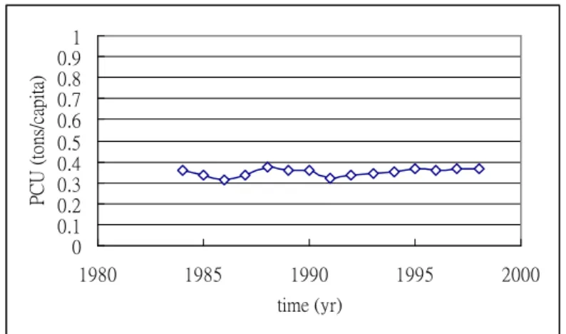
However, the steel industry is also a pollution intensive and energy consuming industry. Consequently, the production of crude steel from the steel industry significantly affects the environment. Figures 4-6 illustrate the yearly variations of the per capita uses (PCUs) of crude steel produced in the U.S.A., Japan, and Taiwan, respectively. The PCU in the U.S.A. holds steady for more than a decade, with relatively low value. The case with Japan is slightly different, with the PCU value much higher than that with the U.S.A.
Moreover, the PCU in Japan shows a slightly downward. On the other hand, the PCU in Taiwan soars at a significantly increasing rate during the same period. According to the above data, the steel industry in Taiwan has grown swiftly. During the same period, the steel industries in the U.S.A. and Japan slowed down or even retreated. Since Taiwan and Japan are export-oriented countries, the needs of steel production in supporting their infrastructures and
manufactures for the exports are significant. This leads to the higher PCUs as compared to that in U.S.A. The results also provide another evidence that the loadings of steel industries are shifted to the less developed countries.
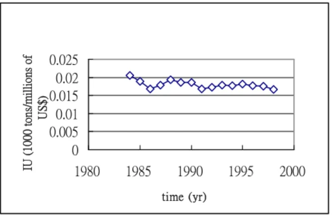
As for the intensities of use (IUs) of the crude steel produced, the results (Figures 7 and 8) indicated that the developed countries such as U.S.A. and Japan demonstrated downward trends, with Japan being the most distinct. The downward trend reflected that the rate of the production of crude steel did not increase in parallel to the increase of GDP. The alter of industry structure and economy might have been the reason. However, this decreasing phenomenon did not emerge in Taiwan. Figure 9 displays that the IU in Taiwan increased after 1995 and the reverse movement between the production of crude steel and GDP did not occur. Thus, Taiwan needed to improve its efficient use of steel and iron in generating high GDP. The increase of IU might not be good for the
environment. Nevertheless, the descending of IU could be the result of advancing in Material Science. More appropriate substitutions may have been found, which drop the consumption of the original materials. When some new substitutions are
merchandised, the production of crude steel may tumble, and the trend of IU would be downward. However, it is not appropriate to assert that the environmental burden reduces as the IU decreases. The environmental impact of the substitutes should be considered in chorus, which requires a life cycle
assessment (LCA).
五
、結論與建議In summary, the proposed dynamic model reasonably depicts the scenario of the IE of Taiwan’s steel industry with the consideration of inventory change via the lumped approach of the steel materials uncollected, discarded, or left in the environment. The model may be applied to other industry sectors with some modification to describe the industrial ecology of target materials.
The yearly variations of the per capita of uses (PCUs) of the steel and iron of steel industries for Japan and U.S.A. show either decreasing or merely constant. However, PCU increases in Taiwan indicating the
increasing need of yearly demand in supporting the development of the country. As for the intensities of use (IUs) of the steel and iron of steel industries, U.S.A. and Japan have the lower IUs and thus the better usages of steel
and iron than Taiwan.
六
、誌謝
This study was supported by the National Science Council of Taiwan under Grant No. NSC90-2621-Z-002-025.
七、符號說明
fI47 Fraction of M7 contributing to Im4 for Approaches 4 to 6, with Im4 = fI47 M7, fI47
=
0.6 forA
pproaches 4 and 5, = 0.1, 0.2, 0.3, 0.4, 0.5, or 0.6 for Approach 6GDP Gross domestic product I Impure material
IE Industrial ecology Im Inventory
Imj Im of Node j, j=1 to 5 Ims ΣImj, j = 1 to 5
Im11 Im of iron ore at Node 1 Im12 Im of crude steel at Node 1 Im13 Im of ferro-alloy at Node 1 Im2 Im of finished steel at Node 2 Im3 Im of consumer goods
manufactured at Node 3
Im4 Im of consumer products for user at Node 4
Im4A3 Im4 for Approach 3
Im4A456 Im4 for Approaches 4 to 6,
= fI47 M7
Im5 Im of scrap at Node 5
Im125 Sum of Im11, Im12, Im13, Im2,
Im5
Im12345 Sum of Im125, Im3, Im4
IISI International Iron and Steel Institute
IU Intensity of use, production/GDP
j Index of node j, j = 1,2,3,4,5 for each node
LCA Life cycle assessment M1 Production of crude steel
M2 Apparent consumption of crude steel
M3 Home scrap
M31 Scrap from Node 1, 0.5 M3 M32 Scrap from Node 2, 0.5 M3 M4 Production of finished product M5 Apparent consumption of
finished product
M6 Production of consumer goods M7 Apparent consumption of
consumer goods M8 Scrap from domestic M9 Production of scrap M10 Consumption of scrap Mce Exported crude steel Mci Imported crude steel Mfe Exported finished steel Mfi Imported finished steel
Mge Exported consumer steel goods Mgi Imported consumer steel goods Mse Exported scrap
Msi Imported scrap
Mun Steel materials uncollected, discarded, or left in the environment
Munj Mun at Node j with j=1 to 5 Muns ΣMunj, j = 1 to 5
P Product
PCU Per capita of use, production/population R Recycled scrap
Rin Iron ore and ferro-alloys into system; taken as iron ore imported
S Salvaged material t Time
TSIIA Taiwan Steel and Iron Institute Association
V Virgin material W Waste
Wc Waste from consumer We Waste from extractor Wm Waste from manufacturer Wr Waste from waste processor β Fraction of output which
becomes Mun
βj Fraction of output in Node j which becomes Munj, j = 1 to 5
八
、參考文獻1. Graedel, T. E. and B. R. Allenby,
Industrial Ecology, Prentice Hall,
Englewood Cliffs, New Jersey (1995). 2. Allenby, B. R. and R. A. Laudise,
“Industrial Ecology— United States,” AT&T Technology, 74(6), 8-17 (1995).
3. Ehrenfeld, J. and N.
Gertler, ”Industrial Ecology in
Practice,” J. Industrial Ecology, 1(1),
67-79 (1997).
4. Korhonen, J., M. Wihersaari and I. Savolainen, “Industrial Ecology of a
Regional Energy Supply System,”
Greener Management International,
26, 57-67 (1999).
5. Wernick I. K., Industrial Ecology and the Built Environment. The Rinker Eminent Scholar Workshop on
Construction Ecology and Metabolism, University of Florida, Gainesville, FL, September 29 (1999).
6. Ruth, M. and P. Dell’Anno, “An Industrial Ecology of the US Glass Industry,” Resources Policy, 23,
109-124 (1997).
7. Sagar, A. D. and R. A. Frosch, “A Perspective on Industrial Ecology and Its Application to a Metal-Industry Ecosysytem,” J. Cleaner Prod., 5,
39-45 (1997).
8. Pento, T., “Industrial Ecology of the Paper Industry,” Wat. Sci. Tech., 40,
21-24 (1999).
9. Wernick, I. K., P. E. Waggoner and J. H. Ausubel, “Searching for Leverage to Conserve Forests-The Industrial Ecology of Wood Products in the United States,” J. Industrial Ecology,
1, 125-145 (1998).
10. Wernick, I. K. and J. H. Ausubel, “National Material Metrics for
Industrial Ecology,” Resources Policy,
21, 189-198 (1995).
11. Cleveland, C. J. and M. Ruth,
“Indicators of Dematerialization and the Materials Intensity of Use,” J. Industrial Ecology, 2(3), 15-50
(1999).
12. TSIIA (Taiwan Steel and Iron Institute Association), Taiwan Steel 2000, TSIIA, Taiwan (2000).
13. IISI (International Iron and Steel Institute), Steel Statistical Year Book, IISI, Belgium (2000).
九、圖說明
Fig. 1. Resources flows in ecosystems. (a) Linear materials flows in “Type I” ecology. (b) Quasi-cyclic materials flows in “Type II” ecology. (c) Cyclic materials flows in “Type III” ecology [1].
Fig. 2. Type II model of industrial metabolic system. Letters refer to the following mass flows: V, virgin material; M, processed material; R, recycled scrap; P, product; S, salvaged material; I, impure material; and W, waste. Flows are sometimes combined in practice. For example, materials processors and recyclers often produce materials ready for transmittal to manufacturers [1]. Fig. 3. Graedel’s Type II material flow model
of steel and iron of Taiwan’s steel industry. Notations: as specified in Tables 1 and 2.
Fig. 4. Production of crude steel /population in U.S.A. Source of data: IISI [13].
Fig. 5. Production of crude steel /population in Japan. Source of data: IISI [13].
Fig. 6. Production of crude steel /population in Taiwan. Source of data: IISI [13].
Fig. 7. IU of crude steel in U.S.A. Base year of US$: 1985. Source of data: IISI [13]. Fig. 8. IU of crude steel in Japan. Base year of
US$: 1985. Source of data: IISI [13]. Fig. 9. IU of crude steel in Taiwan. Base year
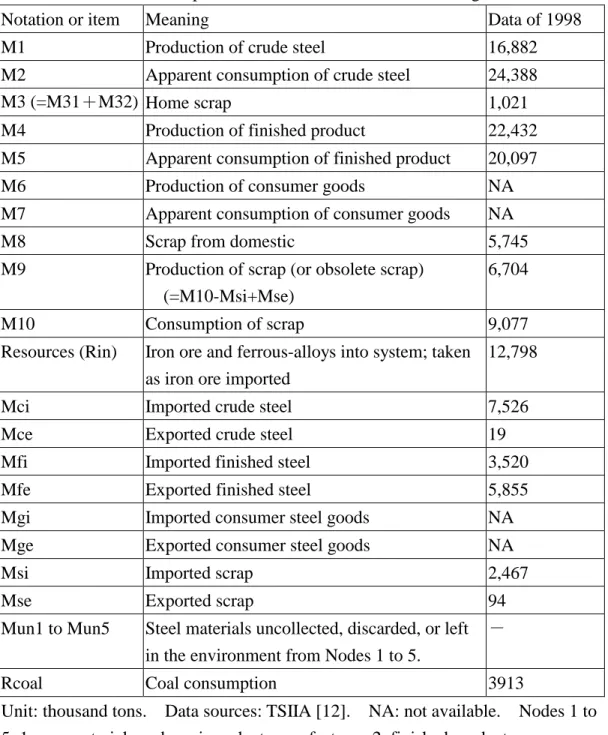
Table 1. Notation explanation and some data of 1998 for Figure 3.
Notation or item Meaning Data of 1998 M1 Production of crude steel 16,882 M2 Apparent consumption of crude steel 24,388 M3 (=M31+M32) Home scrap 1,021 M4 Production of finished product 22,432 M5 Apparent consumption of finished product 20,097 M6 Production of consumer goods NA M7 Apparent consumption of consumer goods NA M8 Scrap from domestic 5,745 M9 Production of scrap (or obsolete scrap)
(=M10-Msi+Mse)
6,704 M10 Consumption of scrap 9,077 Resources (Rin) Iron ore and ferrous-alloys into system; taken
as iron ore imported
12,798 Mci Imported crude steel 7,526 Mce Exported crude steel 19 Mfi Imported finished steel 3,520 Mfe Exported finished steel 5,855 Mgi Imported consumer steel goods NA Mge Exported consumer steel goods NA Msi Imported scrap 2,467 Mse Exported scrap 94 Mun1 to Mun5 Steel materials uncollected, discarded, or left
in the environment from Nodes 1 to 5.
- Rcoal Coal consumption 3913
Unit: thousand tons. Data sources: TSIIA [12]. NA: not available. Nodes 1 to 5: 1. raw materials and semi-product manufacturer, 2. finished product
manufacturer, 3. consumer goods manufacturer, 4. consumer products user, 5. scrap processor.
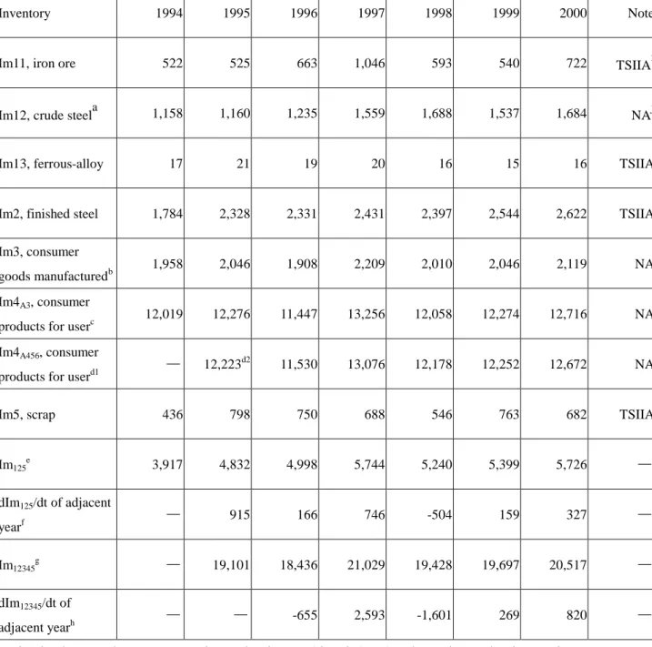
Table 2. Inventories of Nodes 1 to 5 in Figure 3 at the end of the year.
Inventory 1994 1995 1996 1997 1998 1999 2000 Note
Im11, iron ore 522 525 663 1,046 593 540 722 TSIIAi
Im12, crude steela 1,158 1,160 1,235 1,559 1,688 1,537 1,684 NAj
Im13, ferrous-alloy 17 21 19 20 16 15 16 TSIIA
Im2, finished steel 1,784 2,328 2,331 2,431 2,397 2,544 2,622 TSIIA
Im3, consumer goods manufacturedb
1,958 2,046 1,908 2,209 2,010 2,046 2,119 NA
Im4A3, consumer
products for userc
12,019 12,276 11,447 13,256 12,058 12,274 12,716 NA
Im4A456, consumer
products for userd1
-
12,223d2 11,530 13,076 12,178 12,252 12,672 NA
Im5, scrap 436 798 750 688 546 763 682 TSIIA
Im125e 3,917 4,832 4,998 5,744 5,240 5,399 5,726
-
dIm125/dt of adjacent yearf-
915 166 746 -504 159 327-
Im12345g-
19,101 18,436 21,029 19,428 19,697 20,517-
dIm12345/dt of adjacent yearh-
-
-655 2,593 -1,601 269 820-
Unit : in thousand tons. a. Estimated using Im12 = 0.1 M1. b. Estimated using Im3 = 0.1 M5 for Approaches 4 to 6. c. Estimated using Im4 = 0.6 M5 for Approach 3. d1. Estimated using Im4 = fI47M7 = fI47(M5-dIm3/dt) for Approaches 4 to 6, fI47 = 0.6 for
Approaches 4 and 5, fI47 = 0.1, 0.2, 0.3, 0.4, 0.5, or 0.6 for Approach 6. d2. Data for
fI47 = 0.6. e. Sum of Im11, Im12, Im13, Im2, and Im5. f. Data for use in Approaches
1 and 2. g. Sum of Im11, Im12, Im13, Im2, Im3, Im4A456, and Im5. h. Data for use
in Approaches 5 and 6 with fI47= 0.6. i. Data of TAIIA [12]. j. Not available.
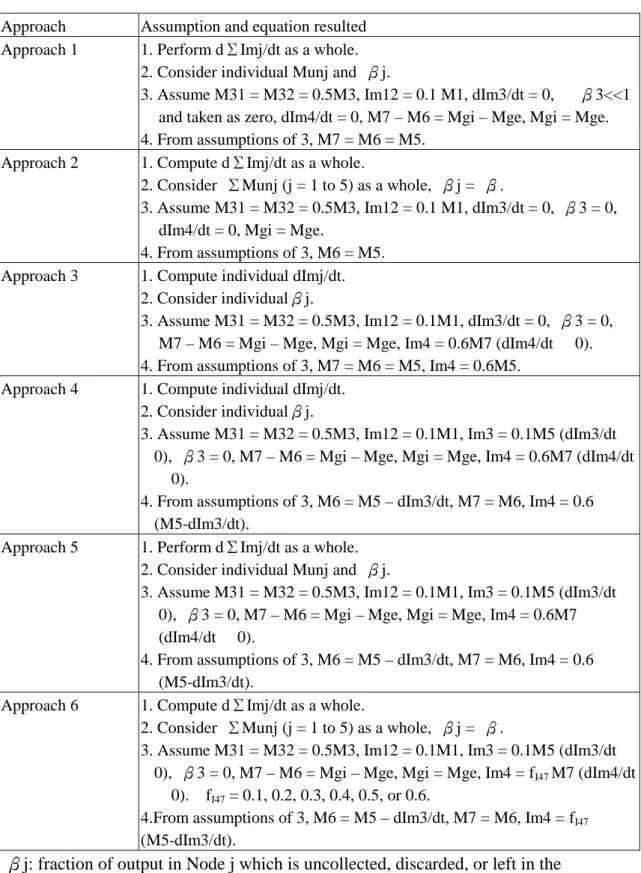
Table 3. Summary of assumptions of different Approaches.
Approach Assumption and equation resulted Approach 1 1. Perform dΣImj/dt as a whole.
2. Consider individual Munj and βj.
3. Assume M31 = M32 = 0.5M3, Im12 = 0.1 M1, dIm3/dt = 0, β3<<1 and taken as zero, dIm4/dt = 0, M7 – M6 = Mgi – Mge, Mgi = Mge. 4. From assumptions of 3, M7 = M6 = M5.
Approach 2 1. Compute dΣImj/dt as a whole.
2. Consider ΣMunj (j = 1 to 5) as a whole, βj = β.
3. Assume M31 = M32 = 0.5M3, Im12 = 0.1 M1, dIm3/dt = 0, β3 = 0, dIm4/dt = 0, Mgi = Mge.
4. From assumptions of 3, M6 = M5. Approach 3 1. Compute individual dImj/dt.
2. Consider individualβj.
3. Assume M31 = M32 = 0.5M3, Im12 = 0.1M1, dIm3/dt = 0, β3 = 0, M7 – M6 = Mgi – Mge, Mgi = Mge, Im4 = 0.6M7 (dIm4/dt 0). 4. From assumptions of 3, M7 = M6 = M5, Im4 = 0.6M5.
Approach 4 1. Compute individual dImj/dt. 2. Consider individualβj.
3. Assume M31 = M32 = 0.5M3, Im12 = 0.1M1, Im3 = 0.1M5 (dIm3/dt 0), β3 = 0, M7 – M6 = Mgi – Mge, Mgi = Mge, Im4 = 0.6M7 (dIm4/dt
0).
4. From assumptions of 3, M6 = M5 – dIm3/dt, M7 = M6, Im4 = 0.6 (M5-dIm3/dt).
Approach 5 1. Perform dΣImj/dt as a whole. 2. Consider individual Munj and βj.
3. Assume M31 = M32 = 0.5M3, Im12 = 0.1M1, Im3 = 0.1M5 (dIm3/dt 0), β3 = 0, M7 – M6 = Mgi – Mge, Mgi = Mge, Im4 = 0.6M7
(dIm4/dt 0).
4. From assumptions of 3, M6 = M5 – dIm3/dt, M7 = M6, Im4 = 0.6 (M5-dIm3/dt).
Approach 6 1. Compute dΣImj/dt as a whole.
2. Consider ΣMunj (j = 1 to 5) as a whole, βj = β.
3. Assume M31 = M32 = 0.5M3, Im12 = 0.1M1, Im3 = 0.1M5 (dIm3/dt 0), β3 = 0, M7 – M6 = Mgi – Mge, Mgi = Mge, Im4 = fI47 M7 (dIm4/dt
0). fI47 = 0.1, 0.2, 0.3, 0.4, 0.5, or 0.6.
4.From assumptions of 3, M6 = M5 – dIm3/dt, M7 = M6, Im4 = fI47
(M5-dIm3/dt).
βj: fraction of output in Node j which is uncollected, discarded, or left in the environment.
Limited waste Energy and limited resources Ecosystem
component Unlimitedwaste Unlimited resources (a) (b) Energy (c) Ecosystem component Ecosysytem component Ecosystem component Ecosystem component Ecosysytem component Ecosystem component Figure 1.
Materials processor or manufacturer Consumer Waste processor Materials extractor or grower We Wm Wc Wr I M S P R W Limited waste Limited resources V Figure 2.
Node 3 Consumer goods
manufacturer Node 1
Raw materials and semiproduct manufacturer Resource M32 Crude steel import Crude steel export Finished steel import Finished steel export Consumer goods import Mun1 M2 M1 M5 Mun3 Scrap export Node 5 Scrap processor Node 4 Consumer products user Consumer goods export Mun4 Mun5 M31 M6 M7 M8 M9 M10 Scrap import Node 2 Finished products manufacturer Mun2 M4 Mce Mci Rin Mse Msi Mge Mgi Mfe Mfi Figure 3.
Figure 4. Figure 5. Figure 6. 0 0.1 0.2 0.3 0.4 0.5 0.6 0.7 0.8 0.91 1980 1985 1990 1995 2000 time (yr) PCU (tons/capita) 0 0.1 0.2 0.3 0.4 0.5 0.6 0.7 0.8 0.9 1 1980 1985 1990 1995 2000 time (yr) PCU (tons/capita) 0 0.1 0.2 0.3 0.4 0.5 0.6 0.7 0.8 0.9 1980 1985 1990 1995 2000 time (yr) PCU (tons/capita)
Figure 7. Figure 8. Figure 9. 0 0.005 0.01 0.015 0.02 0.025 1980 1985 1990 1995 2000 time (yr) IU (1000 tons/millions of US$) 0 0.02 0.04 0.06 0.08 0.1 1980 1985 1990 1995 2000 time (yr) IU (1000 tons/millions of US$) 0 0.02 0.04 0.06 0.08 0.1 1980 1985 1990 1995 2000 time (yr) IU (1000 tons/millions of US$)
行政院國家科學委員會專題研究計畫成果報告
台灣工業生態之調查與研究-砂石、金屬、能源與一事業廢棄物-
子計畫一:
金屬與石化業之工業生態研究及
實施環境管理系統對該產業之環境與經濟效益分析-金屬業 ( I )
第二部份:台灣金屬業實施環境管理系統對該產業之環境與經濟
效益之分析
Part Two: A Study for Impacts of Implementation of Environmental
Management System for Taiwan’s Metal Industry
計畫編號: NSC 90-2621-Z-002-025
執行期間: 90 年 8 月 1 日至 91 年 7 月 31
主持人:何瓊芳(中原大學國際貿易學系)
研究人員:李秀虹、吳胤良
中文摘要
本研究首先針對金屬相關行業已 通過 ISO14001 之 94 家廠商進行問卷調 查 , 並 以 結 構 方 程 模 式 (structural equation modeling) 分 析 各 廠 商 實 施 ISO14001 環境管理系統後,公司在管 理績效、環保、財務績效及整體營運績 效上是否受顯著影響等作深入探討。研 究結果發現在影響管理績效之 14 個因 子中,有 11 個因子達 5%顯著水準,亦 即因為實施 ISO14001,金屬業廠商之 工作環境更符合環保法規要求、處理環 保問題的應變時間縮短、環境目標的達 成率逐年提高、建立了良好的內部環稽 核制度、改善了內部作業程序、有效避 免環保罰款、每年環保總金額及罰單次 數減少、社區關係改善、可降低整體污 染防治設備投資、提昇員工的環保觀 念、良好的工作環境保障員工身心健 康。在環保績效之 14 個影響因子有 12 個達 5%顯著水準,包含節約能源、節 約用水量、空氣污染的減少、水污染的 減少、廢棄物的產生量減少、對土壤污 染的減少、單位產量之廢棄物及污染物 產生率的降低、降低廢棄物的處理時間 及成本、噪音的減少、避免產品的過度 包裝、消耗材再生使用之比例提高、毒 性整化學物質使用量減少等。至於財務 績效方面,雖然全部因子皆不顯著,但 其績效指數亦有 57.28 分(滿分為一百 分)。而對整體績效之 16 個影響因子 中,有 5 個達 5%顯著水準,包含對整 體營運有助益、建立污染管制能力、回 收再利用、節省物料耗用、產品之形象 提升及廢棄物資源化等。研究結果顯示 金屬業實施 ISO14001 環境管理系統 後,除了對財務面之影響不顯著外,在 管理、環保及體營運績效上均具統計顯 著性。而根據結構方程模式分析的結 果,足以顯示模型變數間製程變數、成 本變數及整體營運變數皆受環保變數 影響最甚,而財務變數受成本變數影響 最深。關鍵詞:金屬業、ISO14001、問卷分析 法、線性結構方程模式
Abstract
This study first makes a questionnaire survey on 94 factories that have hold ISO14001 certificate in metal industry. Methods of linear structural relation (LISREL) are then conducted to analyze the effects of ISO certification upon the company’s management administration, environmental protection, public relations, and financial performances. The empirical results show that the holding of ISO certificate has strong positive impacts upon a company’s management administration. The ISO certification also serves to improve a business’ environmental protection as well as public relations. The only weak effect is associated with financial aspect, which may be explained by the purchasing behavior of consumers who are not aware of the content of ISO certification.
Key words: Metal industry, ISO 14001,
questionnaire survey, structural equation modeling 壹、研究背景與動機與流程 人類近百年來對自然資源大量地 開發和利用,使生活和科技水準日新月 異,人類生活更為舒適。但另一方面, 經濟發展的過程中過度開發,使用了大 批的原、物料和能源,亦使自然環境遭 到極大破壞,引起大地的反撲,自 1990 年代起各地洪汛、地震、森林大火,久 旱不雨時有所聞,引起高度環境保護的 關切和訴求。另一方面, 在資源有限 的觀念下,環保意識已然深植人心。從 非經濟層面來看,環保的落實確保了部 分資源之再生利用而使得永續發展的 呼聲不再流為口號,資能源之節用及善 用使地球的資源也能有週而復始的循 環利用得以生生不息;若從社會和經濟 角度來看,許多先進國家的大企業已由 傳統單一追求利潤為最大目標轉為注 重環境管理和求取整體福利二者並行 不 悖 。 國 際 標 準 組 織 (International Organization for Standardization, ISO)1996 年推出之國際環境管理標準 ISO14000 系列,可供全球企業參考並 對我國產業造成重大的衝擊。值得注意 的是台灣在 2002 年 1 月 1 日正式加入 世界貿易組織(World Trade Organization, WTO )後,面對全球性之競爭,台製商 品 走 向 國 際 化 成 為 一 不 可 抑 止 的 趨 勢。除了本身品質要好,市場通路順暢 外,廠商之商品在國際間欲具競爭力, 為配合世界性之環保訴求,廠商取得環 保上的認證將為廠商增加產品之國際 競爭力。 因此,本研究特別探討台灣金屬業 之廠商導入 ISO14000 後對其管理、營 運、環境及財務面之影響性,首先寄發 問卷給金屬業之廠商並將所得之資料 加以量化分析以便於和管理作決策。在 實施 ISO 14000 時能因時因地選擇適合 本身組織模式及行業特性的環境績效 評估指標,並根據這些指標,進行數據 的收集.整理與分析,以提供組織內外的 利害相關者瞭解其所關心之議題。綜合 而言,研究步驟與流程如圖 1-1 所示。 貳、文獻回顧 環境管理系統 ISO14001 之認証及 實施肇始於 1996 年國際標榫組織正式 公佈相關標準後,取得世界性之注意和 認可。其實施結果和成效未探討,仍然 是一個很新的領域,也引起產、官、學 界的研究興趣,分述如下: 黃義俊 (1997) 對中國鋼鐵公司實 施 環 境 管 理 系 統 後 得 到 減 少 工 業 污 染,增加生產效益及員工環境價值觀顯 著提升的績效有報導。許健陞(1997)指 出台灣鋼鐵業員工環保意識、技術訓練 至環境績效的審查,仍有少部分廠商未
予以貫徹。高階主管的投入和鄰近居民 建立良好的溝通,是環境管理系統的必 備條件,就鋼鐵業而言仍有極大空間需 要努力。余瑞華(1999)提出大部分通過 ISO14001 驗證的企業,其實施環境管 理 系 統 (environmental management system, EMS) 的部分大致相同,雖然在 程度上有所不同,但都有益於提升其企 業內部環境管理效益,因為不同的產品 環境考量面資訊來源的証明,會影響企 業內部環境管理效益。 蘇文娟(1999)發現廠商在環境管理 的支出與預算在未來五年將深受其環 境管理推動程度的影響,此亦即意謂廠 商將越來越重視環境管理的課題,並且 願意提供更多的資金來推動環境管理 活動。蘇文娟(1999)更發現現階段業界 在實施環境管理活動後,其效益未能完 全顯現出來,乃由於企業主仍以被動的 態度推行環境管理活動、廠商投入於環 境管理的支出與預算仍不足等因素所 影響。 黃建輝 (1999) 發現林園石化業推 動 ISO14000 環境管理系統之初,有先 期審查評估方式之難處乃在於石化業 製程複雜,所造成的污染與環境影響因 子考量的評估方法不易整合,或是因為 表格繁雜,使執行現場配合意願低。此 外,其要求公司提出具體績效性指標皆 由於涉及公司機密性資料,而有所保 留。
根 據 Proto and Supino (2000) 指 出,ISO14000 環境管理系統在各國施行 的情況至 1999 年 11 月總計有數千家, 義大利從 1996 年至 1999 年雖通過之總 家數只有 422 家,但卻有逐年遞增的趨 勢,顯示該國對環境的重視更加濃厚。 實証發現一組織採用環境管理系統所 能獲得的利益及優勢主要有三:(1)改善 控管其相關環境執行力的能力並能系 統性地紀錄和評估環境的影響性。(2) 透過正式文件的定義而有一較佳的責 任和工作的規範及(3)環境議題與品質 管理的結合可能產生綜效。 Rondinelli (2000) 針 對 美 國 通 過 ISO14001 環 境 管 理 系 統 之 鋁 公 司 (Alumum Mt Holly)進行個案研究,指出 此公司在實施環保政策後有四點明確 的改善,分別為:(1)員工的認知、(2) 營運上的效率(efficiency)、( 3) 經理人 的認知及時行樂、及(4)操作上的效能 (effectiveness)。綜合上述所言,本研究 將相關文獻整理如表 2-1。 參、金屬業之分類及定義 根據行政院主計處 88 年度產業關 聯表之分類,凡製程中包含以下金屬物 料及成品者皆列為本文所欲探討的金 屬業別,詳細資料整理如表 3-1。大體 而言分為 13 類,包含生鐵及粗鋼、鋼 鐵初級製品、鋁、其他金屬、金屬家用 器具、金屬手工具、鋼鐵製品、鋁製品、 其他金屬製品、金屬表面處理、一般通 用機械及金屬加工機械。 肆、研究方法 本研究主要目的,在於探討通過 ISO14001 之金屬業廠商,對其管理績 效、環境保護績效、財務績效及整體績 效上是否有顯著影響。本研究主體上採 用問卷調查法,以通過 ISO14001 之金 屬業廠商為對象,研究對象截至 2002 年 3 月共計 94 家,其中有效樣本為 53 家。問卷內容是利用李克特五點量表 (Likert-type scale)來測定其影響強度。 其 次 , 再 利 用 量 分 結 構 方 程 模 式 (structural equation modeling, SEM) 來 分析各個因子之間的關係及因子中變 數之間的關係。 一、問卷調查 問卷調查是在無明確的數值資料 提供研究者做為數值分析時所採取的 社會科學研究方法,利用問卷所獲得的 一手資料再對其進行量化的分析為本 文所欲探討的重點。本問卷共分為五個
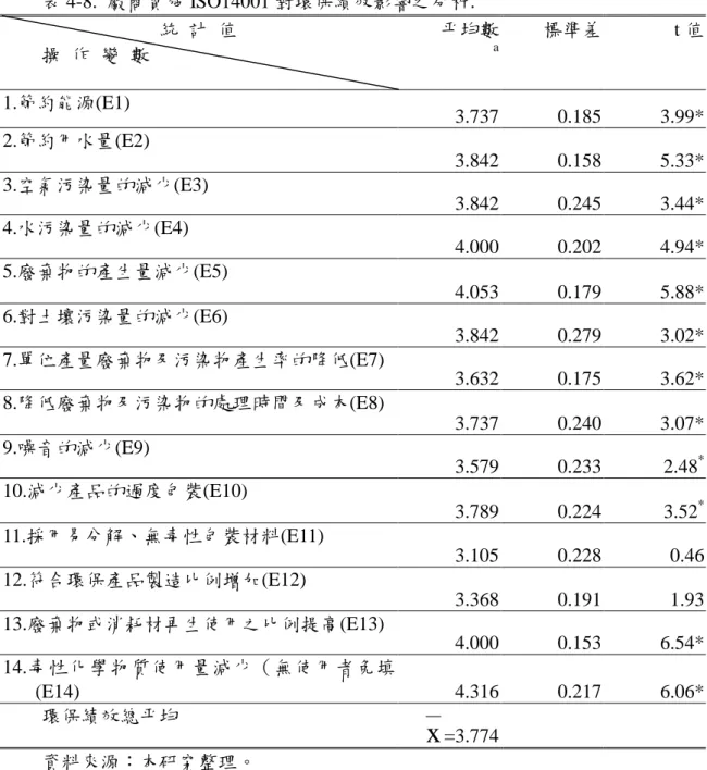
部分:(1)廠商基本資料、(2)管理績效、 (3)環保績效、(4)財務績效、及(5)整體 營運績效。為了得知通過 ISO14001 環 境 管 理 系 統 金 屬 業 廠 商 對 該 產 業 管 理、環保、財務及整體營運績效四方面 的影響度,本問卷採用 5 點李克特量表 進行測量。 (一)問卷之信度與效度分析 1.問卷回收情形 截至 2002 年 3 月 8 日針對金屬業 通過 ISO14001 之廠商寄出問卷,共計 94 家,目前回收之有效樣本計 53 家, 回收率超過半數達 53%。顯示廠商在實 施 ISO14001 環境管理系統後乃持續對 其環境面相關的議題持續關切中。 2.問卷之信度分析 信 度 (Reliability) 是 指 測驗結 果的 一致性或穩定性而言(楊國樞,1993)。 本研究採用 Cronbach’s α係數來檢驗 「 內 在 一 致 信 度 」 (internal consistency)。 根據吳統雄(1984)所建議的信度檢 驗標準如下: (1) α≦0.3:不可信 (2) 0.3<α≦0.4:初步的研究, 勉強可信 (3) 0.4<α≦0.5:稍微可信 (4) 0.5<α≦0.7:可信(最常見的 信度範圍) (5) 0.7<α≦0.9:很可信(次常見 的信度範圍) (6) 0.9<α:十分可信 而 Malhotra (1993)則指出:α係數 在 0.6 以上即表示該問卷達可信的標 準。
本研究以 Statistics for Windows 統 計軟體”STATSOFT”分析問卷之四部分 問項。計算所得 Cronbach’s α值分別 為:管理績效 (management performance indicators, MPI) = 0.901 ; 環 保 績 效 (environment performance indicators,
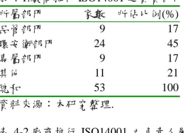
EPI) = 0.903 , 財 務 績 效 (finance performance indicators, FPI) = 0.9731 及 整 體 營 運 (operation performance indicators, OPI) =0.949。問卷所得各問 項 Cronbach’s α 值 均 達 到 吳 統 雄 (1984) ”十分可信” 的分類標準。 3.問卷之效度分析 效度即正確性。指測驗或其他測量 工具確實能測出其所欲測量的特質或 功能 (楊國樞,1993)。本研究問卷內容 來源來自國內外相關文獻整理,並經過 專家修改及鑑定過,以期望建構有效的 內容效度(content validity)。 (二)公司基本資料分析 1.廠商負責推行 ISO14001 的部門 由表 4-1 得知受訪的 53 家廠商 中,其負責執行 ISO14001 工作有 9 家 是為品管部門(佔總回收問卷 17%);24 家為環安衛部門(佔總回收問卷 45%);9 家為專屬部門(佔總回收問卷 17%);有 11 家為其他(佔總回收問卷 21%)。其中 負責的部門大多屬於專業部門,顯示 ISO14001 在廠商內的執行是一種專業 化的過程。 2.廠商推行 ISO14001 負責人層級 由表 4-2 得知受訪的 53 家廠商 中,其推行 ISO14001 的負責人層級 為:有 1 家為公司負責人 (佔總回收問 卷 2%);有 20 家為總經理(副)(佔總 回收問卷 38%);有 7 家為廠長(副)(佔 總回收問卷 13%);有 22 家為經理(副) (佔總回收問卷 42%);有 3 家為其他(佔 總回收問卷 5%)。尤其高階人士如經理 級 以 上 所 佔 的 比 例 高 達 95% , 顯 示 ISO14001 在公司有相當程度的重視。 3.廠商負責推行 ISO14001 的專職人員 數 由表 4-3 得知受訪的 53 家廠商 中,負責推行 ISO14001 的專職人員 數,2 人以下有 21 家(佔總回收問卷 40%);3~5 人有 23 家 (佔總回收問卷 43%);6~10 人有 7 家 (佔總回收問卷
13%);10 人以上有 2 家 (佔總回收問卷 4%)。其中 3~5 人以下負責推行的比例 佔了 83%,顯示推行 ISO14001 是一項 不會耗費太多人力成本的推行工作。 4.廠商的股東組成情況 由表 4-4 得知受訪的 53 家廠商 中,股東組成情況分別為:100﹪外資 的有 3 家 (佔總回收問卷 5%);外資佔 半 數 以 上 有 9 家 ( 佔 總 回 收 問 卷 17%);外資佔半數以下有 11 家 (佔總 回收問卷 21%);全為台資有 30 家(佔總 回收問卷 57%)。顯示不僅台資,連外 商對於環境管理的重視度亦相當高。 5.廠商的製程設備來源 由表 4-5 得知受訪的 53 家廠商 中,其製程設備來源有 27 家來自國內 生產 (佔總回收問卷 39%);有 35 家來 自國外進口 (佔總回收問卷 51%);有 5 家為自行研發 (佔總回收問卷 7%);有 2 家來自其他 (佔總回收問卷 3%)。 6.廠商的內外銷情形 由表 4-6 得知受訪的 53 家廠商 中,其內外銷情形為有 18 家為內銷(佔 總回收問卷 24%);有 35 家為外銷(佔總 回收問卷 76%)。 (三)問卷之管理績效、環保績效、財務 績效及整體營運績效強度檢定 為了得知金屬業廠商對 ISO14001 環境管理系統的看法,本研究針對管 理、環保、財務及整體營運四方面之影 響度,以李克特五點 量表(Likert-type scale)測之。 1.t 檢定 在虛無假設 H0:ì≦3 vs. 對立假 設 H1:ì>3 下,其檢定統計量 t 值為 式(1)
)
x
(
S
x
t
=
−
µ
(1) 其中 x 為 53 家金屬相關廠商之各個方 面變項之平均值,S( x )為其標準差,在 5% 的 顯 著 水 準 下 其 臨 界 值 為 t18, 5%=2.101;其樣本平均值( x )、標準差 (S( x ))和其顯著性整理如下。 2.實施 ISO14001 環境管理系統對管理 績效方面之影響 由表 4-7 得知管理績效項目中除了 M12「與環境考量有關之產品市場佔有 率提昇」、M13「提高顧客的忠誠度」、 及 M14「降低海外市場的進入障礙」不 顯著外,其餘皆達 5% 顯著水準。並且 在 M7「每年環保罰單次數及總金額的 減少」此項目達成的成效最為顯著且強 度最強。由此可推論廠商對於環保的重 視度愈高則收到環保單位的罰款次數 應相對愈少。此一結果可使得未落實環 保的廠商做一參考,並提供其從事環保 工作的誘因。 3. 實施 ISO14001 環境管理系統對環保 績效方面之影響 由表 4-8 得知環保績效項目中除了 E11「採用易分解、無毒性包裝材料」、 及 E12「符合環保產品製造比例增加」 不顯著外,其餘皆為達 5%顯著水準。 顯示廠商在處理污染問題及對於資源 再利用的概念皆已有相當的概念及成 效。 4. 實施 ISO14001 環境管理系統對財務 績效方面之影響 由表 4-9 得知廠商在實施 ISO14001 後在財務績效方面並無顯著影響。值得 注意的是在 F2「每年處理廢棄物及污染 物的費用降低」、F3「減少原料使用(利 用率提高)F5「環保形象增進、公關宣 傳費用降低」、F7「更容易獲得國外廠 商支持」、及 F10「產品競爭力提高」這 幾個項目雖然其所受的影響在 5%顯著 水準下不顯著,但確實有較高的觀察值 (大於 3),而且由於其為一平均值,是 故可推論的確有部分廠商在此已達到 相對的財務成效,而其乃為實施環境管 理系統後之成效。5.實施 ISO14001 環境管理系統對整體 營運績效方面之影響 由表 4-10 得知整體營運績效項目 中除了 O9「建立污染管制能力」、O10 「重複使用、回收再利用、節省物料耗 用」、O12「產品之形象提升」、及 O14 「廢棄物資源化、價值化」在 5%顯著 水準下達顯著外,其餘皆不顯著。 6.問卷綜合比較分析 由圖 4-1 知管理績效、環保績效、 財務績效、及整體營運績效之總體平均 值分別為 3.88、3.774、2.864、及 3.165(滿 點為 5)。可知管理績效之成效為最高, 其次為環保績效,整體營運績效為第 三,並且以上三者皆大於理論平均值 3。而財務績效之平均值為 2.846,並且 在 5%顯著水準下,顯著不大於理論平 均值 3。將此四項績效指標加總平均 後,所得總績效為 3.421 乃大於 3,顯 示廠商在實施 ISO14001 環境管理後, 雖然在某些個別項目上會有不明顯的 影響,但對整體績效來看仍不失為一正 面性的影響。 根據上述統計結果,吾人可推論: 廠商在推行 ISO14001 環境管理系統 後,確實在管理、環保、財務、及整體 營運績效上有其一定的影響度,並且皆 為正面的助益。大體而言,管理績效之 影響度最大,其次為環保績效,再其次 為整體營運上的績效,而財務上的績效 雖最為薄弱,其績效指數亦有 57.28 分 (滿分為一百分)。顯示 ISO14001 環境管 理系統有其推行的必要性。 二、結構方程模式分析 (一)結構方程模式變數設計、假設及模 型之建立 根據陳正昌與程炳林(1998)指出 在 LISREL (linear structure relation)模式 中計有 4 種變項,分別為 2 種潛在變項 和 2 種觀察變項:在潛在變項中,被假 定 為 因 者 稱 為 潛 在 自 變 項 (latent independent variable) 或 稱 為 外 衍 變 項 (exogenous variable),被假定為果者的 潛 在 變 項 稱 做 潛 在 應 變 項 (latent dependent variable) 或 稱 為 內 衍 變 項 (endogenous variable)。同理,2 種觀察 變項亦被假定為一因一果。本研究採用 陳正昌與程炳林(1998)的分類法將其 整理如表 4-11 及表 4-12,並分類如下: 1.自變數的觀察變項:將問卷之第二部 份至第四部份即管理績效指標、環保 績效指標及財務績效指標,個別依其 屬性分為外在變數(MO、EO、FO)、 內在變數(MI、EI、FI)及影響性變 數(ME、EE、FE)等三項,作為自 變數的觀察變項(即假定為因者)。 2.應變數的觀察變項:將問卷之第五部 分即整體營運績效指標分為創新程 度變數(Y1)、生產效能變數(Y2)、 市場佔有率變數(Y3)、獲利能力變 數(Y4)、資源再利用率變數(Y5)、 人力資源變數(Y6)、物料成本變數 (Y7)、污染管制變數(Y8)、企業 與產品形象變數(Y9)及整體營運效 益變數(Y10)計十項,作為應變數 的觀察變項(即假定為果者)。 3.自變數的潛在變項:將管理績效的內 在、外在與影響三項變數,整合為管 理面變數(M)。環保績效的內在、 外在與影響三項變數,整合為環保面 變數(E)。財務績效的內在、外在與 影響三項變數,整合為財務面變數 (F)。此三項變數作為自變數的潛在 變項(即假定為因者)。 4.應變數的潛在變項:將問卷第五部分 之整體營運績效之問項依其同質度 將創新程度與生產效能歸為製程面 變數(Process)。市場佔有率、獲利 能力與資源再利用率歸為獲利面變 數(Profit)。人力資源與物料成本歸 為成本面變數(Cost)。企業與產品 形象、污染管制與整體營運效益歸為 營運效益的變數(Operation)。此四 項變數作為應變數的潛在變項(即假 定為果者)。 本文為相關性(correlation)研究。
Borg and Gall (1989) 提及相關性研究 的目的是藉由相關係數統計來探索變 數之間的關係。本研究利用結構方程模 式處理因子間彼此之因果關係。有關 SEM 的軟體相當多,本文利用 LISREL 8.30 for Window 套裝軟體來分析之,它 是由瑞典學家 JÖ reskog and SÖ rbom (1993a)所設計。根據陳順宇(1998)描 述 LISREL 主要探討變數間的線性關 係,並對可觀測的(顯性)變數與不可 觀測的(隱性)變數的因果模式進行假 設檢定。而有關模式適配度的評鑑, Bagozzi and Yi (1988)認為可從基本的 適配(preliminary fit criteria)、模型內在 結構適配度(fit of internal structural of model) 整體模 型適 配 度 (overall model fit) 三方面來評量。其中「基本適配標 準」是用來檢測模型之誤差、辨識或輸 入有誤等問題;「模型內在結構適配度」 是 在 評 量 模 型 內 估 計 參 數 的 顯 著 程 度,各指標及潛在變項的信度;而「整 體模型適配度」是用來測定整體模型與 觀 察 資 料 的 適 配 程 度 。 本 文 綜 合 Bagozzi and Yi (1998)及陳順宇(1998)的 評量法,將評鑑指標歸納如表 4-13. 本文依據表 4-11 及 4-12 所陳述各 因子之關係利用 LISREL 模式之徑路圖 繪製如圖 4-2 所示,其中箭頭所指為果 而箭頭起源處為因,而根據本研究的目 的,本文提出 13 個研究假設以利提議 模型(proposed model)之分析: 假設 1:此模型存在因果關係 假設 2:通過 ISO14001 金屬業廠商之 管 理 面 變 數 (M) 對 其 製 程 面 變 數 (process)有顯著且正面的影響 假設 3:通過 ISO14001 金屬業廠商之 管理面變數(M)對其獲利面變數(profit) 有顯著且正面的影響 假設 4:通過 ISO14001 金屬業廠商之 管理面變數(M)對其成本面變數(cost) 有顯著且正面的影響 假設 5:通過 ISO14001 金屬業廠商之 管 理 面 變 數 (M) 對 其 營 運 面 變 數 (operation)有顯著且正面的影響 假設 6:通過 ISO14001 金屬業廠商之 環 境 面 變 數 (E) 對 其 製 程 面 變 數 (process)有顯著且正面的影響 假設 7:通過 ISO14001 金屬業廠商之 環 境 面 變 數 (E) 對 其 獲 利 面 變 數 (profit)有顯著且正面的影響 假設 8:通過 ISO14001 金屬業廠商之 環境面變數(E)對其成本面變數(cost) 有顯著且正面的影響 假設 9:通過 ISO14001 金屬業廠商之 環 境 面 變 數 (E) 對 其 營 運 面 變 數 (operation)有顯著且正面的影響 假設 10:通過 ISO14001 金屬業廠商之 財 務 面 變 數 (F) 對 其 製 程 面 變 數 (process)有顯著且正面的影響 假設 11:通過 ISO14001 金屬業廠商之 財務面變數(F)對其獲利面變數(profit) 有顯著且正面的影響 假設 12:通過 ISO14001 金屬業廠商之 財務面變數(F)其成本面變數(cost)有 顯著且正面的影響 假設 13:通過 ISO14001 金屬業廠商之 財 務 面 變 數 (F) 對 其 營 運 面 變 數 (operation)有顯著且正面的影響 (二)LISREL 模式分析結果 本文之 LISREL 使用金屬樣本資料 的相關矩陣作為資料的輸入方式,所得 結果整理如表 4-14
至 4-16.
由表 4-16結果顯示與前述 LISREL 評鑑模式指標相比,表 4-16 整體模式 適 合 度 準 則 中 之 Chi-square 值 為 4653.809 (自由度為 134),並且在 1%的 顯著水準下,達到顯著,此結果未達判 斷準則標準 (p 值大於 0.05),但根據樊 愛群與周子敬 (2001) 一文提及由於樣 本數對於 ÷2太敏感,特別是樣本數超過 200 的時候。Hair 等人(1998)亦強調,“ ÷2 值在大樣本及小樣本時都太敏感了,研 究分析者需要伴隨其他適配測量值來 辨別模式的適配度。” 其他 2 個衡量的指標為適配度指數(goodness-of-fit, GFI) 及 殘 差 平 方 根 (root mean square residual, RMR),本文 提議模式之 GFI 是 0.674,RMR 為 0.083。Hair 等人(1998)指出 GFI 值越 高,適配性越好,但是模式接受性的臨 界並沒有確切的底定下來,GFI 指數的 最大值為 1,但有可能出現負值。雖然, Hair 等人 (1998) 提及並沒有確切值以 接受模式,但一般學者提出的臨界值為 0.9。 RMR 是適配殘差變異數/共變數平 均值的平方根,故其值越小,表示模式 的適配性越佳。根據樊愛群與周子敬 (2001) 一文提及,分析矩陣若是相關矩 陣,則 RMR 必須低於 0.05,最好是低 於 0.025 。 而 調 整 後 適 配 度 指 數 (adjusted goodness-of-fit index, AGFI), 及 NFI (normed fit index) 在所提議的模 型 中 都 小 於 判 斷 標 準 0.9 而 分 別 為 0.537 及 0.761。 綜合整體模式適配度測量,可以知 道提議模式僅能達到 Hair 等人 (1998) 提議的邊緣支援模式,但仍需進一步加 以檢視測量模式、結構模式以及進行模 式修改的動作。 依據圖 4-2 及表 4-14 及 4-15 之分 析數據對照,整個 LISREL 模式之驗證 結果可以圖 4-3 表示.圖 4-3 之分析結 果,可分為衡量性模式與結構性模式, 以 分 別 探 討 其 在 模 式 假 設 上 的 適 當 性。衡量模式包括管理面變數(M)、 環保面變數(E)、財務面變數(F)、製 程 面 變 數 ( Process )、 獲 利 面 變 數 (Profit)、成本面變數(Cost)、營運效 益面變數(Operation),七個變數之建構 分析。 在管理面變數(M)的建構上,以 管理績效指標的外在變數(λMO=0.833) 為最大的影響因素,其影響因子包含環 境更符合環保法規要求(M1)、處理環保 問題的應變時間縮短(M2)、有效避免環 保罰款(M6)、每年環保罰單次數及總金 額的減少(M7)、社區關係的改善(附近 居民的抱怨或索賠次數降低)(M8);其 次 為 管 理 績 效 指 標 的 影 響 變 數(λME =0.830),其影響因子包含良好的工作環 境保障員工身心健康(M11)、與環境考 量有關之產品市場佔有率提昇(M12)、 提高顧客的忠誠度(M13)、降低海外市 場的進入障礙(M14);再者為管理績效 指標的內在變數(λMT =0.636),其影響 因子包含環境目標的達成率逐年提高 (M3)、建立了良好的環保內部稽核制度 (M4)、改善內部作業程序(M5)、降低未 來整體污染防治設備投資(M9)、提昇員 工的環保觀念(M10)。 在環保面變數(E)的建構上,以 環保績效指標的內在變數(λEI=0.884) ) 為最大的影響因素,其影響因子包含節 約能源(E1)、節約用水量(E2)、單位產 量廢棄物及污染物產生率的降低(E7)、 降低廢棄物及污染物的處理時間及成 本(E8)、減少產品的過度包裝(E10)、廢 棄 物 或 消 耗 材 再 生 使 用 之 比 例 提 高 (E13);其次為環保績效指標的影響變數 (λEE=0.867),其影響因子包含空氣污染 量的減少(E3)、水污染量的減少(E4)、 廢棄物的產生量減少(E5)、對土壤污染 量的減少(E6)、噪音的減少(E9);再者 為 環 保 績 效 指 標 的 外 在 變 數 ( λ EO=0.666),其影響因子包含採用易分 解、無毒性包裝材料(E11)、符合環保產 品製造比例增加(E12)、毒性化學物質使 用量減少。 財務面變數(F)的建構上,以財 務績效指標的外在變數(λFO=0.940), 為最大的影響因素,其影響因子包含賦 稅減免(投資優惠)(F1)、貸款取得更 容易(F6)、更容易獲得國外廠商支持 (F7)、增加政府獎助的機會(F9)、爭取 更佳的信用條件(可延遲付款)(F18)、 關 於 環 保 方 面 之 營 業 外 收 益 提 高 (F19);其次為財務績效指標的影響變數 (λFE=0.922),其影響因子包含環保形象 增進、公關宣傳費用降低(F5)、創新、 專利可能獲利(F8)、產品競爭力提高