在量子計算機上電路滿足問題的最佳化的分子解的最佳化的量子演算法

行政院國家科學委員會專題研究計畫 成果報告

在量子計算機上電路滿足問題的最佳化的分子解的最佳化

的量子演算法

研究成果報告(精簡版)

計 畫 類 別 ： 個別型

計 畫 編 號 ： NSC 97-2221-E-151-035-

執 行 期 間 ： 97 年 08 月 01 日至 98 年 07 月 31 日

執 行 單 位 ： 國立高雄應用科技大學資訊工程系暨研究所

計 畫 主 持 人 ： 張雲龍

計畫參與人員： 碩士班研究生-兼任助理人員：謝東諺

碩士班研究生-兼任助理人員：張又文

大專生-兼任助理人員：陳柏樺

報 告 附 件 ： 出席國際會議研究心得報告及發表論文

處 理 方 式 ： 本計畫可公開查詢

中 華 民 國 98 年 10 月 19 日

行政院國家科學委員會補助專題研究計畫 □成果報告

在量子計算機上

電路滿足問題的最佳化的分子解的最佳化的量子演算法

計畫類別：□ 個別型計畫

計畫編號：NSC 97-2221-E-151 -035

執行期間：97年 08月 01日至 98年 07月 31日

計畫主持人：張雲龍 教授

共同主持人：陳碧慧

計畫參與人員：張又文、謝東諺、陳柏樺

成果報告類型(依經費核定清單規定繳交)：□精簡報告

本成果報告包括以下應繳交之附件：

□出席國際學術會議心得報告及發表之論文各一份

處理方式：除產學合作研究計畫、提升產業技術及人才培育研究計畫、

列管計畫及下列情形者外，得立即公開查詢

□立即公開查詢

執行單位：國立高雄應用科技大學資訊工程系暨研究所

中

華 民 國 9 8 年 1 0 月 0 1 日

Abstract—In this paper, we demonstrate that the logic

computation performed by the DNA-based algorithm for solving general cases of the satisfiability problem can be implemented more efficiently by our proposed quantum algorithm on the quantum machine proposed by Deutsch. To test our theory, we carry out a three-qubit NMR experiment for solving the simplest satisfiability problem.

Index Terms—Quantum Algorithms, Molecular Algorithms,

the NP-Complete Problems, the Satisfiability Problem.

I. INTRODUCTION

ince the publication of Deutsch’s [1] and Adleman’s [2] seminal articles, various quantum algorithms and DNA-based algorithms have been, respectively, proposed for many computational problems. So far, the most frequently cited quantum algorithms are Shor’s algorithms for solving factoring integers and discrete logarithm [3] and Grover’s search algorithm [4] for unsorted databases. On the other hand, famous DNA-based algorithms are used to solve factoring integers [5] and the set-partition problem [6].

II. QUANTUM ALGORITHMS FOR BIO-MOLECULAR SOLUTIONS OF THE SATISFIABILITY PROBLEM

A. All of the Possible Solutions to the Satisfiability Problem

A clause is a formula of the form un ∨ un − 1 … ∨ u2 ∨ u1, where

each uk for 1 ≤ k ≤ n is a Boolean variable or its negation. In

general, a satisfiability problem includes a Boolean formula of the form C1 ∧ C2 … ∧ Cm where each Cj for 1 ≤ j ≤ m is a clause.

Then, the question is to find values of the variables so that the Manuscript received April 23, 2007; revised May 13, 2008. This work was partly supported by the National Science Foundation of R. O. C. under Grants No. 96-2221-E-151-008- and 96-2218-E-151-004-, and also partly supported by the National Natural Science Foundation of China under Grants No. 10774163 and No. 2006CB921203.

Weng-Long Chang and Kawuu Weicheng Lin are with the Department of Computer Science and Information Engineering, National Kaohsiung University of Applied Sciences, Taiwan, R.O.C. (fax: +886-7-3837424; e-mail: [email protected], [email protected]).

Ting-Ting Ren, Jun Luo, Mang Feng are with State Key Laboratory of Magnetic Resonance and Atomic and Molecular Physics,Wuhan Institute of Physics and Mathematics, Chinese Academy of Sciences, Wuhan, 430071, People’s Republic of China (e-mail: [email protected], [email protected], [email protected]).

Minyi Guo is with the School of Computer Science and Engineering, University of Aizu, Fukushima 965-8580, Japan. (e-mail: [email protected]). Copyright (c) 2008 IEEE.

whole formula has the value 1.

Assume that U is a set of 2n _{possible choices and equal to {u} n

un − 1 … u2 u1| ∀ uk ∈ {0, 1} for 1 ≤ k ≤ n} and each element

represents one of 2n _{combinational states for n Boolean}

variables. For the sake of presentation, we suppose that uk

0 _is

used to denote the value of uk to be zero and uk

1 _{means value of}

uk to be one. The jth element in U can be represented as a

unique computational state vector u₁ =

[

n

]

_n , 2 1 2 , 1 2 , 1 1 , 1 T u u u × L where u_{1 ,j} = 1, ∀ u_{1 ,h} = 0 for 1 ≤ h ≠ j ≤ 2n. The corresponding computational state vector for the first element, un

0 _u

n − 1

0 _{… u}

20 u10, in U is

[

1 0 L 0

]

_1×2nT, and the corresponding computational state vector for the last element, un1 un − 11 … u21 u11, in U is

[

0 0 L 1

]

_1×2nT. For the sake of presentation, we assume that B is the set of the corresponding computational state vectors to the elements in U and B = {

[

1 0 L 0

]

_1×2nT …

[

0 0 L 1

]

_1×2nT }. Because each component in B is a coordinated vector, we span

B = C2n[1, 3, 4], where C2n is a Hilbert space. This implies

that the set B is an orthonormal basis in a Hilbert space.

B. Computational Space of Molecules for the Satisfiability Problem

The following bio-molecular operations cited from [2] will be used to construct computational space of molecules for solving the satisfiability problem with m clauses and n Boolean variables.

Definition 2−1: Given a set U = {un un − 1 … u2 u1| ∀ uk ∈ {0, 1}

for 1 ≤ k ≤ n}and a Boolean variable uj, the bio-molecular

operation, “Append-Head”, appends uj onto the head of every

element in the set U. The formal representation is written as Append-Head(U, uj) = {uj un un − 1 … u2 u1| ∀ uk ∈ {0, 1} for 1 ≤

k ≤ n and uj ∈ {0, 1}}.

Definition 2−2: Given a set U = {un un − 1 … u2 u1| ∀ uk ∈ {0, 1}

for 1 ≤ k ≤ n}and a Boolean variable uj, the bio-molecular

operation, “Append-Tail”, appends uj onto the end of every

element in the set U. The formal representation is written as Append-Tail(U, uj) = {un un − 1 … u2 u1 uj| ∀ uk ∈ {0, 1} for 1 ≤

k ≤ n and uj ∈ {0, 1}}.

Definition 2−3: Given a set U = {un un − 1 … u2 u1| ∀ uk ∈ {0, 1}

for 1 ≤ k ≤ n}, the bio-molecular operation, “Discard(U)” sets U

Quantum Algorithms for Bio-molecular

Solutions of the Satisfiability Problem

on a Quantum Machine

S

to be an empty set.

Definition 2−4: Given a set U = {un un − 1 … u2 u1| ∀ uk ∈ {0, 1}

for 1 ≤ k ≤ n}, the bio-molecular operation “Amplify(U, {Ui})”

creates a number of identical copies, Ui, of the set U, and then

discard(U).

Definition 2−5: Given a set U = {un un − 1 … u2 u1| ∀ uk ∈ {0, 1}

for 1 ≤ k ≤ n} and a Boolean variable, uj, if the value of uj is

equal to one, then the bio-molecular extract operation creates two new sets, +(U, uj

1_{) = {u}

n un − 1 … uj

1 _{… u}

2 u1| ∀ uk ∈ {0, 1}

for 1 ≤ k ≠ j ≤ n}and −(U, uj

1_{) = {u}

n un − 1 … uj

0 _{… u}

2 u1| ∀ uk ∈

{0, 1} for 1 ≤ k ≠ j ≤ n}. Otherwise, it produces another two new sets, +(U, uj

0_{) = {u} n un − 1 … uj 0 _{… u} 2 u1| ∀ uk ∈ {0, 1} for 1 ≤ k ≠ j ≤ n}and −(U, uj 0_{) = {u} n un − 1 … uj 1 _{… u} 2 u1| ∀ uk ∈ {0, 1} for 1 ≤ k ≠ j ≤ n}.

Definition 2−6: Given m sets U1 … Um, the bio-molecular

merge operation, ∪(U1, …, Um) = U1 ∪ … ∪ Um.

Definition 2−7: Given a set U = {un un − 1 … u2 u1| ∀ uk ∈ {0, 1}

for 1 ≤ k ≤ n}, the bio-molecular operation “Detect(U)” returns a true if U ≠ ∅. Otherwise, it returns a false.

Definition 2−8: Given a set U = {un un − 1 … u2 u1| ∀ uk ∈ {0, 1}

for 1 ≤ k ≤ n}, the bio-molecular operation “Read(U)” performs an arbitrary element in U. Even if U contains many different elements, the bio-molecular operation can give an explicit description of exactly one of them.

For solving the satisfiability problem with m clauses and n Boolean variables, the following bio-molecular algorithm can be used to create all of the 2n _{possible choices. A set U is an}

empty set and is regarded as the input set of the DNA-based algorithm. The second parameter n in CombinationalStates(U,

n) is to represent the number of Boolean variables.

Procedure CombinationalStates(U, n) (0a) Append-Tail(U1, un 1_). (0b) Append-Tail(U2, un 0_). (0c) U = ∪(U1, U2). (1) For k = n − 1 downto 1 (1a) Amplify(U, U1, U2). (1b) Append-Tail(U1, uk 1_). (1c) Append-Tail(U2, uk 0_). (1d) U = ∪(U1, U2). End For End Procedure

Lemma 2−1: For solving the satisfiability problem with m

clauses and n Boolean variables, 2n _{possible choices created}

from the DNA-based algorithm, CombinationalStates(U, n), form an orthonormal basis of a Hilbert space (i.e., a complex vector space, 2n).

C

C. Computational Space of Quantum Mechanical Solution for the Satisfiability Problem

A qubit (quantum bit) has two ‘computational basis vectors’ 0 and 1 of the two-dimensional Hilbert space corresponding to the classical bit values 0 and 1 [1, 3, 4], and an arbitrary state ϕ of a qubit is a linearly weighted combination

of the computational basis vectors (2.1): ϕ = l1 ⋅ 0 + l2 ⋅ 1 ,

where the weighted factors l1 and l2 ∈ C2 are the so-called

probability amplitudes, with | l1 |2 + | l2 |2 = 1. A collection of n

qubits is called a qregister (quantum register) of size n. It may include any of the 2n_{-dimensional computational basis vectors,}

n qubits of size, or arbitrary superposition of these vectors [1, 3,

4].

D. Lipton’s DNA-based Algorithms of Solving the Satisfiability Problem

Lipton’s DNA-based algorithm [7] for solving the satisfiability problem is described below. The symbol |Cj| in the

following algorithm is applied to represent the number of Boolean variables and their negations in the jth clause in a formula.

Algorithm 2−1: Lipton’s DNA-based algorithm for solving the

satisfiability problem.

(1) CombinationalStates(U, n) (2) For j = 1 to m do begin (3) For i = 1 to |Cj| do begin

(4) If the ith element in the jth clause is one of n Boolean variables uk, Then (5) Ui = +(U, uk 1_{) and U = −(U, u} k 1₎ (6) Else (7) Ui = +(U, uk 0_{) and U = −(U, u} k 0₎ (8) End If (9) End For (10) Discard(U) (11) For i = 1 to |Cj| do begin (12) U = ∪(U, Ui) (13) End For (14) End For

(15) If (Detect(U) = = true) Then (15a) Read(U)

EndIf

(16) End Algorithm

Lemma 2−2: Algorithm 2−1, Lipton’s DNA-based algorithm,

can be applied to solve the satisfiability problem with m clauses and n Boolean variables.

E. Introduction of Quantum Gates for Solving the Satisfiability Problem

The time evolution of the states of quantum registers can be modeled by means of unitary operators which are often referred to as quantum gates [1, 3, 4]. Therefore, a quantum gate can be regarded as an elementary quantum-computing device which performs a fixed unitary operation on selected qubits during a fixed period of time. The NOT gate is a one-qubit gate and sets the only (target) bit to its negation. The CNOT (controlled

NOT) gate is a two-qubit gate and flips the second qubit (the

target qubit) if and only if the first qubit (the control qubit) is one. The CCNOT (controlled-controlled-NOT) gate is a three-qubit gate and flips the third qubit (the target qubit) if and only if the first qubit and second qubit (the two control qubits) are both one.

F. Constructing Quantum Networks for Solving the Satisfiability Problem

The operations OR and AND are implemented by quantum circuits in Figures 2−1 and 2−2, respectively. For evaluating a clause with the form un ∨ un − 1 … ∨ u2 ∨ u1, three quantum

registers unL u1 , ynL y1 and rnrn−1Lr1r0 are

needed. Therefore, its evaluating computation is equal to (2.2):

1 1 r r r_{n n− L} r₀ y_nL y₁ u_nL u₁ → ) ( ) (r_n⊕y_n•r_n−1 L r₁⊕y₁•r₀ r0 ynL y1 unL u1 ,

where

•

denotes operation AND of their negations of two Boolean variables {y_k ,r_k−1} for 1 ≤ k ≤ n. The first bit, r0, in the

third quantum register is initially prepared in state 0 and , other n bits in the third quantum register are initially prepared in state 1 The (n + 1)th quantum bit, r. n, in the third register is

employed to store the final result of the evaluating computation.

Figure 2−1: OR operation of two Boolean variables.

Figure 2−2: AND operation of two Boolean variables. Then, in order to evaluate AND operation of the previous clause and the current clause, the fourth quantum register

0 1

1 c c

c

c_{m m− L} is needed. The first bit, c0, in the fourth

quantum register is initially prepared in state ,1 and other m bits in the quantum register are initially in state 0 The (m + . 1)th quantum bit, cm, in the fourth register is employed to store

the final result of evaluating computation for all of the clauses. The full network, QEC (the abbreviation of quantum evaluating circuit for checking whether the current clause is true or not), is illustrated in Figure 2−3 in Appendix A and can be understood as follows:

• We compute the (n + 1)th bit of the third quantum register to the final result of evaluating a clause. This step requires computing all the OR operations through the relation rk ←

rk ⊕ (yk•rk−1) for 1 ≤ k ≤ n. Then, we compute AND

operation of the previous clause and the current clause through the relation cj ← cj ⊕ (cj−1•rn) for 1 ≤ j ≤ m.

• Subsequently we reverse all those OR operations in order to restore every quantum bit of each quantum register to its

initial state. This enables us to reuse the same quantum registers, should the problem, for example, require repeated

OR operation.

Subsequently, we reverse all those operations (NOT or

CNOT) on the second quantum register to restore every

quantum bit of the second quantum register to its initial state. This enables us to reuse the same second quantum register to evaluate the next clause.

G. Quantum Algorithms of Lipton’s DNA-based Algorithms for Solving the Satisfiability Problem

Based on Algorithm 2−1 in Subsection D, the following quantum algorithm is proposed to work on the physical quantum computer proposed by Deutsch [1]. For convenience of our following presentation, we suppose that cj

1 _{denotes the}

value of cj to be 1 and cj

0_{defines the value of c}

j to be 0 for 1 ≤ j

≤ m. We also assume that rk

1 _{denotes the value of r}

k to be 1 and

rk

0_{defines the value of r}

k to be 0 for 0 ≤ k ≤ n. Similarly, yk

1

denotes the value of yk to be 1 and yk

0_{defines the value of y}

k to

be 0. Moreover, the notations used in Algorithm 2−2 below have been denoted in previous subsections.

Algorithm 2−2: Quantum algorithms of Lipton’s DNA-based

algorithm for solving the satisfiability problem with m clauses and n Boolean variables.

(1) For an input Φ = ) ( 1 0 s m s= c ⊗ ⊗( 1 ) 0 c ⊗(⊗1_q=n r_q1 ) ⊗(r₀0 )⊗(⊗1_q=n y_q0 )⊗ ), ( 1 0 q n q= u

⊗ 2n _{possible choices of n bits (including all of the}

possible choices) are ϕ_{1 ,0} = ( 1 _{2 2})

× = ⊗_{s m}I ⊗ (I2×2) ⊗ ( 1 _{2 2}) × = ⊗_{q n}I ⊗ (I2×2) ⊗ (⊗1q=nI2×2) ⊗ H ⊗n _{Φ =} n 2 1 ) ( 1 0 s m s= c ⊗ ⊗ ( 1 ) 0 c ⊗ (⊗1_q=n r_q1 ) ⊗ (r₀0 ) ⊗ ) ( 1 0 q n q= y ⊗ ⊗( 1 ( 0 1 )). q q n q u + u ⊗ = (2) For j = 1 to m do begin (3) For i = 1 to |Cj| do begin

(4) If the ith element in the jth clause is one of n Boolean variables uk, Then (5) ϕ_{j ,i} = ( 1 _{2 2}) × = ⊗_{s m}I ⊗ (I2×2) ⊗ (⊗1q=nI2×2) ⊗ (I2×2) ⊗ ( 1 _{2 2}) × + = ⊗k I n p ⊗ ( ( ) ) 1 0 0 k k k u u y ⊕ + ⊗ (⊗1_p=k−1I_2×2) ⊗ ) ( 1 _{2 2} × = ⊗_{q n}I ϕ_{j ,i−1} = n 2 1 ) ( 0 s j m s= c ⊗ ⊗ ( 1 ) 1 s j s= − c ⊗ ⊗ ( 1 ) 0 c ⊗ (⊗1_q=n r_q1 ) ⊗ ) ( 0 0 r ⊗ ( 1 p0 ) k n p y + = ⊗ ⊗ ( 0 1 ) k k y y + ⊗ (⊗1p=k−₁ yp0 ) ⊗ )), ( ( 1 0 1 q q n q u + u ⊗ = where . 1 1 for ) ( ₁• − ≥ ≥ ⊕ =c c₋ r j s cs s s n (6) Else (7) ϕ_{j ,i} = ( 1 _{2 2}) × = ⊗_{s m}I ⊗ (I2×2)⊗ (⊗1q=nI2×2) ⊗ (I2×2)⊗

) ( 1 _{2 2} × + = ⊗k I n p ⊗ _{1 0} ) ( ) ) 1 0 ( ( 0 0 1 2 2 k k k u u y ⊕ + ⎟⎟ ⎠ ⎞ ⎜⎜ ⎝ ⎛ × ⊗ ( 1 _{2 2}) 1 × − = ⊗_{p k} I ⊗ (⊗1q=nI2×2) ϕj ,i−1 = n 2 1 ) ( s0 j m s= c ⊗ ⊗ ( 1 ) 1 s j s= − c ⊗ ⊗ ( 1 ) 0 c ⊗ (⊗1q=n rq1 ) ⊗ ) ( 0 0 r ⊗ ( k 1 _p0 ) n p y + = ⊗ ⊗ ( 1 0 ) k k y y + ⊗ (⊗1_p=k−1 y_p0 ) ⊗ ( 1 ( 0 1 )), q q n q u + u ⊗ ₌ where . 1 1 for ) ( ₁• − ≥ ≥ ⊕ =c c₋ r j s c_{s s s n} (8) End If (9) End For (10) ϕ_{j+1,- 1} = QEC ⊗ ( 1 _{2 2}) × = ⊗_{q n}I j C j, ϕ = n 2 1 ) ( 1 0 s j m s c + = ⊗ ⊗ ( c_j⊕(c_j−1•r_n) ) ⊗ (⊗1_s=j−1c_s ⊗ ) ( 1 0 c ⊗ (⊗1q=n rq1 ) ⊗ ( ) 0 0 r (⊗1q=nYq ) ⊗ )), ( ( 1 0 1 q q n q u + u

⊗ ₌ where QEC is the quantum evaluating circuit for checking whether the current clause is true or not in Figure 2−3 in Appendix A, , 1 1 for ) ( 1• − ≥ ≥ ⊕ =c c− r j s cs s s n and . negation a is it if riable Boolean va a is it if 0 1 1 0 ⎪⎩ ⎪ ⎨ ⎧ + + = q q q q q y y y y Y (11) ϕ_{j+1 ,0} = ( 1 _{2 2}) × = ⊗_{s m}I ⊗ (I2×2) ⊗ (⊗1q=nI2×2) ⊗ (I2×2) ⊗ ( 1 ) q n q= V ⊗ ⊗ ( 1 _{2 2}) × = ⊗_{q n}I ⊗ ϕ_{j+1 ,-1} = n 2 1 ) ( 1 0 s j m s c + = ⊗ ⊗ ( 1 ) s j s= c ⊗ ⊗ ( 1 ) 0 c ⊗ (⊗1_q=n r_q1 ) ⊗ ) ( 0 0 r (⊗1q=n yq0 ) ⊗ ( ( )), 1 0 1 q q n q u + u ⊗ = where 1 for ) ( ₁• ≥ ≥ ⊕ =c c₋ r j s c_{s s s n} and ⎪ ⎪ ⎪ ⎩ ⎪⎪ ⎪ ⎨ ⎧ + ⊕ ⎟⎟ ⎠ ⎞ ⎜⎜ ⎝ ⎛ + ⊕ = × × . negation its : )) ( ( 0 1 1 0 riable Boolean va a : ) ( clause in the appearance no : 1 0 2 2 1 0 2 2 q q q q q q q u u Y u u Y I V (12) End For

(13) We obtain the final result, ϕ_m+1,1 , after a measurement of . 0 , 1 + m ϕ End Algorithm

Lemma 2−3: Algorithm 2−2 is a quantum treatment for

Lipton’s DNA-based algorithm, which can be used to solve the satisfiability problem with m clauses and n Boolean variables.

Proof:

Because there are 2n _{possible choices for the satisfiability}

problem with m clauses and n Boolean variables, a quantum register of n bits ( 1 )

k n q= u

⊗ is employed to represent 2n

choices with initial state ( 1 0 )

q n q= u

⊗ . The satisfiability problem with m clauses and n Boolean variables is to evaluate whether the whole formula has the value 1, so three auxiliary quantum registers are needed. The initial states of these auxiliary quantum registers are ( 1 0 ),

q n q= y ⊗ ) ( 1 1 q n q= r ⊗ ⊗ ( 0 ) 0 r and (⊗1_s=m c_m0 ) ⊗

(

c

1₀

)

, respectively. Therefore, the total Hilbert space is (⊗s = m1 C2) ⊗

C2 ⊗ (⊗q = n1 C2) ⊗ C2 ⊗ (⊗q = n1 C2) ⊗ (⊗q = n1 C2).

From the execution of Step (1), an initial vector Φ = ) ( 1 0 m m s= c ⊗ ⊗ ( 1 ) 0 c ⊗ (⊗1_q=n r_q1 ) ⊗ (r₀0 ) ⊗ (⊗1_q=n y_q0 ) ⊗ ( 1 0 ) q n q= u

⊗ starts the quantum computation of the satisfiability problem. H⊗n that stands for the joined n-qubit Hadamard gate is applied to the part of choices of the initial vector Φ then the resulting state vector becomes , ϕ_{1 ,0} = n 2 1 ) ( 1 0 m m s= c ⊗ ⊗ ( 1 ) 0 c ⊗ (⊗1_q=n r_q1 ) ⊗ (r₀0 ) ⊗ ) ( 1 0 q n q= y ⊗ ⊗( 1 ( 0 1 )). q q n q u + u ⊗ =

Step (2) is the outer loop of the main loop and is to judge whether each clause in m clauses is true or not. Step (3) is the first inner loop of the main loop and is used to test whether the

jth clause with 1 ≤ j ≤ m is true or not. On each execution of

Step (4), if the ith element in the jth clause is one of n Boolean variables uk, then this implies that those choices with the value

1 of uk satisfy the jth clause and thus the operation CNOT

) ) ( ., . ( 0 0 1 k k k u u y e

i ⊕ + corresponds to the implementation of

Step (5) in Algorithm 2−1. Otherwise, from each execution of Step (6) the ith element in the jth clause is its negation and this implies that those choices with the value 0 of uk satisfy the jth

clause, and hence the operation NOT and CNOT ) ) ( ) 0 1 1 0 ( ., . ( 0 0 1 2 2 k k k u u y e i _⎟⎟ ⊕ + ⎠ ⎞ ⎜⎜ ⎝ ⎛ × corresponds to the implementation of Step (7) in Algorithm 2−1. After repeating the Steps (4) to (7), we have

j

C j ,

ϕ including those choices that satisfy the jth clause and those illegal choices that dissatisfy the jth clause.

Next, each execution of Step (10) works as the unitary operator, QEC, that is the quantum circuit in Figure 2−3 in Appendix A to judge whether the jth clause is true or not and whether both the (j − 1)th clause and the jth clause are true or not. On each execution of Step (11), the initial state of the first auxiliary quantum register is reset to be ( 1 0 )

q n q= y

⊗ . This

implies that the Step (10) through Step (13) in Algorithm 2−1 have been done. After repeating each operation embedded in the main loop, we get the resulting state vector ϕ_{m+1 ,0}

including those choices that satisfy the whole formula and those illegal choices that dissatisfy the whole formula.

Finally, based on 1 ,

m

c the execution of Step (13) is for a

measurement to find the answer to the satisfiability problem with m clauses and n Boolean variables. Therefore, Algorithm

2−2, i.e., quantum algorithm of Lipton’s DNA-based algorithm,

can also be used to solve the satisfiability problem with m clauses and n Boolean variables. J

III. QUANTUM IMPLEMENTATION OF A BIO-MOLECULAR COMPUTING ON A QUANTUM

MACHINE

The following lemmas are introduced to show that the bio-molecular computer proposed by Adleman [2] can be implemented on the quantum machine proposed by Deutsch [1].

Lemma 3−1: For any NP-complete problem, 2n possible

solutions on the bio-molecular computer proposed by Adleman [2] can be implemented on the quantum machine proposed by Deutsch [6], where n is the number of bits for input size of the problem.

Proof:

From Lemma 2−1, 2n _{possible solutions, U = {u}

n un − 1 … u2

u1| ∀ uk ∈ {0, 1} for 1 ≤ k ≤ n}, for any NP-complete problem

are created from the DNA-based algorithm,

CombinationalStates(U, n). From Lemma 2−1, 2n possible

solutions form an orthonormal basis of a Hilbert space (a complex vector space, 2n).

C Similarly, 2n possible quantum

solutions for the same problem are φ = H⊗n _{00L =} 0

n 2 1 , 1 2 0

∑

− = n i

i and also form an orthonormal basis of a Hilbert space (a

complex vector space, 2n).

C Therefore, from the statements

above, we may conclude that for any NP-complete problem, 2n

possible solutions on the bio-molecular computer proposed by Adleman [2] can be implemented on the quantum machine proposed by Deutsch [1]. J

Lemma 3−2: The bio-molecular operation, Append-Head(U, uj)

= {uj un un − 1 … u2 u1| ∀ uk ∈ {0, 1} for 1 ≤ k ≤ n and uj ∈ {0,

1}}, denoted in Definition 2−1 can be implemented by the corresponding quantum operator, Φ = 0 ⊗ (H⊗n _000L0) = 0 ⊗ ( n 2 1

∑

− = 1 2 0 n i i ) or Φ = 1 ⊗ (H⊗n _000L0) = 1 ⊗ ( n 2 1

∑

− = 1 2 0 n i i ). Proof:

From Definition 2−1, for 2n _{possible solutions U = {u} n un − 1

… u2 u1| ∀ uk ∈ {0, 1} for 1 ≤ k ≤ n} and a Boolean variable uj,

the bio-molecular operation, “Append-Head”, appends uj onto

the head of the elements in the set U, that is, Append-Head(U,

uj) = {uj un un − 1 … u2 u1| ∀ uk ∈ {0, 1} for 1 ≤ k ≤ n and uj ∈ {0,

1}}. If the value for uj is equal to 0, then from Lemma 3−1, the

action of the bio-molecular operation “Append-Head” can be implemented by Φ = 0 ⊗ (H⊗n _{000L0) = 0 ⊗ (} n 2 1

∑

− = 1 2 0 n i

i ). Otherwise, the action of the bio-molecular operation

“Append-Head” can be implemented by Φ = 1 ⊗ (H⊗n _000L0) = 1 ⊗ ( n 2 1

_∑

− = 1 2 0 n i i ). J

Lemma 3−3: The bio-molecular operation, Append-Tail(U, uj)

= {un un − 1 … u2 u1 uj| ∀ uk ∈ {0, 1} for 1 ≤ k ≤ n and uj ∈ {0,

1}}, denoted in Definition 2−2 can be implemented by Φ = (H⊗n _000L0) ⊗ 0 = ( n 2 1

∑

− = 1 2 0 n i i ) ⊗ 0 or Φ = (H⊗n _000L0) ⊗ 1 = ( n 2 1

∑

− = 1 2 0 n i i ) ⊗ 1 .

Proof: Refer to Lemma 3−2. J

Lemma 3−4: The bio-molecular extract operation, +(U, uj

1_{) =}

{un un − 1 … uj

1 _{… u}

2 u1| ∀ uk ∈ {0, 1} for 1 ≤ k ≠ j ≤ n}and −(U,

uj

1_{) = {u}

n un − 1 … uj

0 _{… u}

2 u1| ∀ uk ∈ {0, 1} for 1 ≤ k ≠ j ≤ n},

denoted in Definition 2−5 can be implemented by CNOT.

Proof: Refer to Algorithm 2−2. J

Lemma 3−5: The bio-molecular extract operation, +(U, uj

0_{) =}

{un un − 1 … uj

0 _{… u}

2 u1| ∀ uk ∈ {0, 1} for 1 ≤ k ≠ j ≤ n}and −(U,

uj

0_{) = {u}

n un − 1 … uj

1 _{… u}

2 u1| ∀ uk ∈ {0, 1} for 1 ≤ k ≠ j ≤ n},

denoted in Definition 2−5 can be implemented by NOT and

CNOT

Proof: Refer to Algorithm 2−2. J

Lemma 3−6: Assume that U = {un un − 1 … u2 u1| ∀ uk ∈ {0, 1}

for 1 ≤ k ≤ n} and W is a subset of U and Ua is also a subset of U

for 1 ≤ a ≤ m. From Definition 2−3 and Definition 2−6, the bio-molecular merge operation and discard operation, i.e., ∪(U1, …, Um) = U1 ∪ … ∪ Um and Discard(W) = ∅, perform

logic computation of the satisfiability problem that can be implemented by NOT, CNOT, CCNOT.

Proof: Refer to Algorithm 2−2. J

Lemma 3−7: Assume that U = {un un − 1 … u2 u1| ∀ uk ∈ {0, 1}

for 1 ≤ k ≤ n}. From Definition 2−7 and Definition 2−8, the bio-molecular detect operation and read operation, i.e., Detect(U) and Read(U), to find the answer to the satisfiability problem can be implemented by means of measurements.

Proof: Refer to Algorithm 2−2. J

Theorem 3−1: The bio-molecular computer proposed by

Adleman [2] is a subset of the quantum machine proposed by Deutsch [1] and can be implemented on the quantum machine.

Proof:

From Lemmas 3−1 through 3−7, it is very clear that bio-molecular computational space for any NP-complete problem can be constructed on a quantum machine, and the

bio-molecular operations proposed by Adleman [2] can also be implemented by quantum gates (NOT, CNOT, and CCNOT). Therefore, it is inferred that the bio-molecular computer proposed by Adleman [2] is a subset of the quantum machine proposed by Deutsch [1] and can be implemented on the quantum machine. J

Theorem 3−2: For those famous NP-complete problems that

had been solved on a bio-molecular computer, their corresponding DNA-based algorithms can be fully implemented on a quantum machine.

Proof:

From Theorem 3−1, it is very obvious that a bio-molecular computer can be implemented on a quantum machine. Therefore, it is derived at once that the DNA-based algorithms of solving those famous NP-complete problems can be all implemented on a quantum machine. J

IV. COMPLEXITY ASSESSMENT

The following lemmas could be used to show the time complexity and space complexity of Algorithm 2−2 for solving the satisfiability problem with m clauses and n Boolean variables

Lemma 4−1: Time complexity of solving the satisfiability

problem with m clauses and n Boolean variables is O(n) Hadamard gates, O(10 × m × n) NOT gates, O(2 × m × n)

CNOT gates, O(2 × m × n + m) CCNOT gates, and O(1)

projective operators.

Proof:

In Step (1) of Algorithm 2−2, n Hadamard gates are performed. Next, Step (5) and Step (7) of Algorithm 2−2 are embedded in the main loop, corresponding to the implementation of at most (m × n) NOT gates and (m × n)

CNOT gates. From Step (10) of Algorithm 2−2, we have (8 ×

m × n) NOT gates and (2 × m × n + m) CCNOT gates

performed and Step (11) leads to at most (m × n) NOT gates and (m × n) CNOT gates. Finally, Step (13) of Algorithm 2−2 is a one projective operator. So, time complexity is O(n) Hadamard gates, O(10 × m × n) NOT gates, O(2 × m × n)

CNOT gates, O(2 × m × n + m) CCNOT gates, and O(1)

projective operators. J

Lemma 4−2: Space complexity of solving the satisfiability

problem with m clauses and n Boolean variables is O(m + 3 × n + 2) quantum bits.

Proof:

From Step (1) in Algorithm 2-2, it is indicated that the total Hilbert space is (⊗s = m 1 _C2_{) ⊗ C}2 _{⊗ (⊗} q = n 1 _C2_{) ⊗ C}2 _{⊗ (⊗} q = n 1 C2) ⊗ (⊗q = n

1 _C2_{). So, the space complexity is O(m + 3 × n + 2)}

quantum bits. J

V. AN EXAMPLE OF THREE-QUBIT SOLUTION FOR THE SATISFIABILITY PROBLEM

Consider the formula: F = (u1), the simplest case of the

satisfiability problem. It contains one clause “(u1)”, and one

Boolean variable u1. The following algorithm, i.e., Algorithm

5−1, is the reduced version of Algorithm 2−2 in Subsection F

and is employed to find the answer of the satisfiability problem of the clause, F = (u1).

Algorithm 5−1: Solving the satisfiability problem of the clause,

F = (u1).

(1) For an input Φ = 0 1

c ⊗ y₁0 ⊗ u₁0 , two choices are 0 , 1 ϕ = (I2×2) ⊗ (I2×2) ⊗ (H) Φ = 2 1 ( 0 1 c ) ⊗ ( y10 ) ⊗(u₁0 + u₁1 ). (2) ϕ_{1 ,1} = (I2×2) ⊗ (y10⊕(u10+u11) ) ⊗ (I2×2) ϕ1 ,0 = 2 1 ( 0 1 c ) ⊗( y₁0+y₁1 ) ⊗ (u₁0 + u₁1 ). (3) ϕ_{2 ,-1} = ( ( 1) ) 1 0 1 0 1 y y c ⊕ + ⊗ (I2×2) ⊗ (I2×2) ϕ1 ,1 = 2 1 ) ) ( ( 1 1 0 1 c c + ⊗(y₁0+y₁1 )⊗ (u₁0 + u₁1 ). (4) ϕ_{2 ,0} = (I2×2) ⊗(( ) ( 11) ) 1 1 0 1 0 1 u y u y ⊕ + ⊕ ⊗ (I2×2) ϕ2 ,-1 = 2 1 ) ) ( ( 1 1 0 1 c c + ⊗ ( y₁0 ) ⊗ (u₁0 + u₁1 ).

(5) We obtain the final result, ϕ_2,1 , after a measurement of . 0 , 2 ϕ End Algorithm

So, from Step (1) of Algorithm 5−1, for an input Φ =

0 1

c ⊗ y₁0 ⊗ u₁0 , 21 possible choices are ϕ_{1 ,0} =

2 1 ( 0

1

c y₁0 u₁0 + c₁0 y₁0 u₁1 ). Then, in the first

clause, the first Boolean variable is u1. Therefore, after the Step

(2) of Algorithm 5−1 is performed, we have ϕ1 ,1 =

2 1 ( c₁0 y₁0 u₁0 + c₁0 y₁1 u₁1 ). Because only a clause

and a Boolean variable are involved in the example, we could use CNOT gate to replace QEC in Figure 2−3 in Appendix A to evaluate whether the only clause with the only Boolean variable is true or not. Hence, the implementation of Steps (3) and (4) in Algorithm 5−1 yields ϕ_{2,- 1} =

2 1 ( c₁0 y₁0 0 1 u + c₁1 y₁1 u₁1 ) and ϕ_{2 ,0} = 2 1 ( 0 1 c y₁0 0 1

u + c₁1 y₁0 u₁1 ). Step (5) of Algorithm 5−1 is for a

measurement on ϕ_{2 ,0} to find c₁1 , i.e., the answer to the

satisfiability problem for the formula: F = (u1). The

measurement yields ϕ_{2 ,1} = 1 1

c y₁0 u₁1 , and the

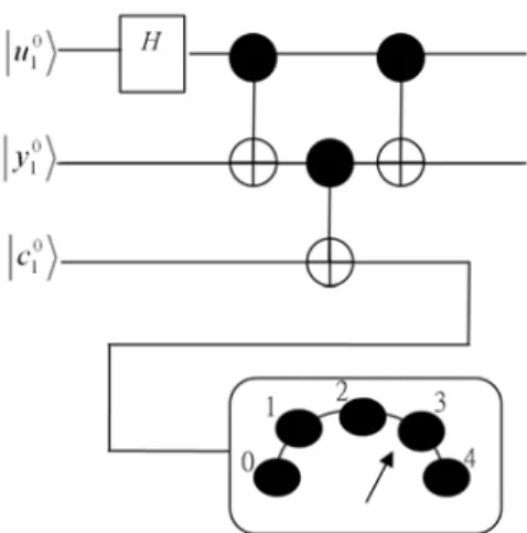
corresponding quantum circuit of the example above is shown in Figure 5-1.

Figure 5-1: The quantum circuit of the example above. NMR approach has been widely employed to quantum information processing over past years due to its mature and well-controllable technology. Although the quantum information processing by NMR is made on ensembles of nuclear spins, instead of individual spins, NMR has remained to be the most convenient experimental tool to demonstrate quantum information processing. We here also adopt this technology to check our theory.

Our experiment is carried out on a Varian INOVA 600 NMR spectrometer. The sample is 13C−labelled _{alanine with}

formula 131CH3−132CH NH( 2)−133COOH _{, where the three}

carbons 131C,132C,133C _{correspond to the qubits} I I1, , 2 I3 _,

respectively. The J-coupling constants are J12=34.79Hz J, 23=54.01Hz J, 13=1.20Hz . Selective excitation was achieved by using soft pulses.

The experiment has three main steps as follows:

Step 1 is for initialization. Before the algorithm is carried out, the initial state, i.e., the pseudo-pure state, must be well prepared. There have been many methods to do this job, among which the spatial averaging method proposed by Cory et al. is most commonly used. So in our experiment, we have also employed this technique to prepare the three-qubit pseudo-pure state for which the detailed pulse sequence can be found in. The states of the input qubits are prepared by following operation

1z 2z 3z 21z 2z 2 2z 3z 21z 3z 41z 2z 3z

E I+ +I +I + I I + I I + I I + I I I _{, where E is}

the unity operator with the form of

1 0 0 1 E= ⎜⎛ ⎞_⎟ ⎝ ⎠_{, and} 1 2 iz z I = σ , with

i = 1, 2 and 3, being the ith spin angular momentum operator in

the z direction, and σz is the Pauli matrix,

1 0 0 1

z

σ _{= ⎜}⎛ ₋ ⎞⎟ ⎝ ⎠_.

Step 2 translates the quantum gates into NMR pulses, respectively. We had to connect and optimize the pulses to construct the total NMR pulse sequence. The Hadamard gate can be achieved by a single π/2 pulse with phase x. The

CNOT gate can be implemented by NMR pulses as follows,

2 1,2 1,2 2

[ / 2]π y→(1/ 4 )J →[ ]π x →(1/ 4 )J →[ ]π x →[ / 2]π x, where the

flip angle of the pulse and the time of delay are written in the

square brackets and in the round brackets, respectively. The subscripts are the phases (i.e., along the x or y axis) of the pulse, and the superscripts are the nuclei to which the pulses are applied. Then we could obtain the total pulse sequence by connecting and optimizing the above pulses according to the quantum circuit.

Step 3 is the measurement, where a readout pulse is applied to each qubit to obtain the spectra.

Note that in NMR measurements, the frequencies and phases of NMR signals could clearly indicate the state the system evolved to after the readout pulses have been applied. In our experiment, the phases of the reference of 13

C spectra from a

thermal equilibrium was adjusted to be in absorption (i.e., to be positive), and then the same phase corrections were used to determine the absolute phases of the experimental spectra of the 13

C after the algorithm is accomplished. In our case, the

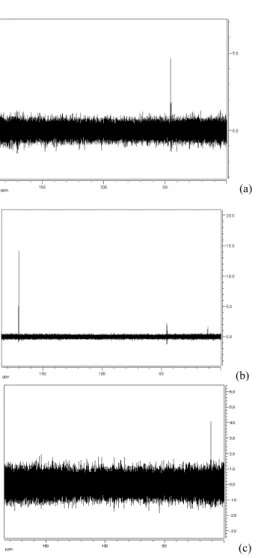
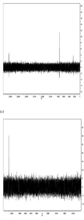
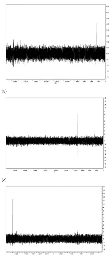
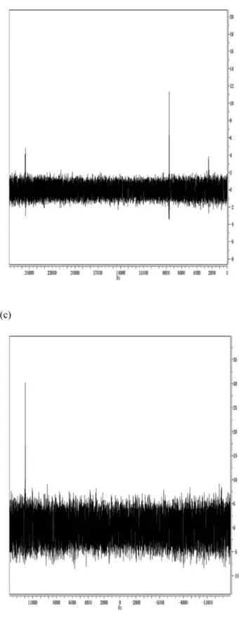
final state was 2 / 0 | ) 11 | 00 (| 2 / ) 101 | 000 (| 〉₁₂₃+ 〉₁₂₃ = 〉₁₃+ 〉₁₃ 〉₂ , which means the first and the third qubits are entangled. As the readout by NMR is a weak measurement, we have no state collapse after the measurement. Besides, only single quantum coherence can be detected in NMR. As a result, we have to employ some additional operations for detecting the output state (|000>+|101>)/ √ 2. We may detect the second qubit directly by applying a π/2 readout pulse along the x axis, yielding Figure 5-2 (b). But for the first and third qubits, we need to disentangle them before measurement. To this end, we apply a CNOT gate, respectively, on the first and second qubits followed by another CNOT gate, respectively, on the second and first qubits to get the state (|000>+|011>)/√2. Then the first qubit can be read out by a single π/2 pulse along the x axis, as shown in Figure 5-2 (a). Similar steps applied to the third qubit result in the spectrum in Figure 5-2 (c). It is evident that the experimental results are in good agreement with our theoretical prediction.

Therefore, due to the fact that NMR quantum operations are not made on individual nuclear spins, but on spin ensemble, there is a difference in the operation between Figure 5-1 and our experiment. Some remarks must be addressed. First of all, the three-qubit NMR experiment we have carried out suffices to make a comprehensive test for our theory, because we have achieved the key aspects of our theory. Although the simple case with three qubits did not reflect the efficiency of quantum computation for SAT problem, we argue that, with more variables and clauses involved, the quantum computing efficiency would be more and more evident, which has been reflected in our above discussion about the computational complexity. Secondly, DNA computation does not involve entanglement, whereas entanglement does appear in our quantum treatment. The necessity of additional operations to disentangle the output qubits is not the intrinsic characteristic of our quantum mechanical treatment, but due to the unique feature of NMR technique. Anyway, those additional operations have not changed the essence of our implementation.

(a)

(b)

(c)

Figure 5-2: The experimental spectra (a), (b) and (c) of the

three-qubit solution for satisfiability problem after the readout on the first, second and third qubits, respectively.

VI. CONCLUSIONS

By using the mature technique of NMR, we have carried out a solution for the simplest satisfiability problem. The experimental results are in well agreement with the theoretical prediction.

REFERENCES

[1] D. Deutsch, “Quantum theory, the Church-Turing principle and the universal quantum computer,” Proceeding of Royal Society of London series A, 400, 97-117, 1985.

[2] L. Adleman, “Molecular computation of solutions to combinatorial problems,” Science, 266: 1021-1024, 1994.

[3] P. W. Shor, “Algorithm for quantum computation: discrete logarithm and factoring algorithm,” Proceedings of the 35th Annual IEEE Symposium on

Foundation of Computer Science, 124-134, 1994.

[4] L. K. Grover, “A fast quantum mechanical algorithm for database search,”

Proceedings of the twenty-eighth annual ACM symposium on Theory of computing, 212-219, 1996.

[5] W.-L. Chang, M. Ho and M. Guo.,“Fast Parallel Molecular Algorithms for DNA-based Computation: Factoring Integers,” IEEE Transactions on

Nanobioscience, Vol. 4, No. 2, pp. 149-163, 2005.

[6] Weng-Long Chang, “Fast Parallel DNA-based Algorithms for Molecular Computation: the Set-Partition Problem,” IEEE Transactions on

Nanobioscience, Vol. 6, No. 1, pp. 346-353, 2007.

[7] R. Lipton, “DNA Solution of Hard Computational Problems,” Science, 268: pp.542-545, 1995.

APPENDIX A

Figure 2−3: The full network is the QEC (the abbreviation of quantum evaluating circuit) to check whether the current clause is true or not.

Abstract—In this paper, quantum algorithms for solving an

instance of the subset-sum problem is proposed and a NMR experiment for the simplest subset-sum problem to test our theory is also performed.

I. INTRODUCTION

I

n this paper, an instance of the subset-sum problem can be implemented by our proposed quantum algorithm. By using nuclear magnetic resonance (NMR) technique, we perform an

NMR experiment for the simplest subset-sum problem to test

our theory.

II. QUANTUM ALGORITHMS OF THE SUBSET-SUM PROBLEM

A. Definition of the Subset-sum Problem

Assume that a finite set A is {a1, …, am}, where ak is the kth

element for 1 ≤ k ≤ m. Definition 4−1 is applied to denote the subset-sum problem for any a finite set, A.

Definition 4−1: The subset-sum problem for an m-element

finite set, A, is to find a subset A1 _{⊆ A such that the sum of}

every element in A1 _{is exactly b, where b is any given positive}

integer.

B. Computational State Space of Quantum Solutions for the Subset-sum Problem

An arbitrary state

ϕ

of a quantum bit is nothing else than a linearly weighted combination of the following computational basis vectors (4.1):

ϕ

= l1 ⋅

0

+ l2 ⋅

1

=

l1 ⋅ 1 2

0

1

×

⎥

⎦

⎤

⎢

⎣

⎡

+ l2

,

1

0

1 2×

⎥

⎦

⎤

⎢

⎣

⎡

where the weighted factors l1 and l2 ∈

C2 are the so-called probability amplitudes, thus they must

satisfy | l1 |2 + | l2 |2 = 1.

C. Introduction of Quantum Gates for Solving the Subset-sum Problem

The NOT gate is a one-qubit gate and sets the only (target) bit to its negation. The CNOT (controlled NOT) gate is a two-qubit gate and flips the second qubit (the target qubit) if Weng-Long Chang is with Department of Computer Science and Information Engineering, National Kaohsiung University of Applied Sciences Kaohsiung City, Taiwan 807-78, Republic of China (e-mail: [email protected]).

Mang Feng was with State Key Laboratory of Magnetic Resonance and Atomic and Molecular Physics, Wuhan Institute of Physics and Mathematics, Chinese Academy of Sciences, Wuhan, 430071, People’s Republic of China (e-mail: [email protected]).

and only if the first qubit (the control qubit) is one. The

CCNOT (controlled-controlled-NOT) gate is a three-qubit

gate and flips the third qubit (the target qubit) if and only if the first qubit and second qubit (the two control qubits) are both one.

D. Constructing Quantum Networks for Solving the Subset-sum Problem

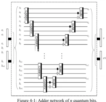
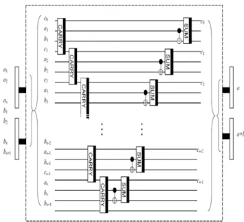
The full addition network is illustrated in Figure 4-1, and can be understood as follows:

Figure 4-1: Adder network of n quantum bits. We only reverse all these operations in Figure 4-1 in order to restore every quantum bit of the three registers to its initial state. This enables us to reuse the same registers repeatedly.

E. Quantum Algorithms of Solving the Subset-sum Problem

The following quantum algorithm is proposed as quantum implementation on a physical quantum. The notations used in

Algorithm 4-1 below have been denoted in previous

subsections.

Algorithm 4-1: The quantum algorithm is to solve an instance

of the subset-sum problem for any given positive integer b with a finite set A involving m elements of n bits.

(1) For an initial input

ϕ

₀ =

(

⊗

1_p=_n

r

_p0

)

⊗

(

)

1 0

r

⊗

)

(

1 _{1 ,} 1 q n q= +

b

⊗

⊗

(

b

_n+10

)

⊗

(

⊗

1j=n

b

j0

)

⊗

)

(

0 , 1 1 ,j n k j m k= =

a

⊗

⊗

(

0

)

1 , 1 1 ,= − =

⊗

_{k m j n}

c

_{k j} ⊗

Quantum Algorithms of the Subset-sum Problem on a Quantum Computer

)

(

1 0 k m k=

e

⊗

⊗

(

0

)

1 + n

r

⊗

(

1

),

2m _{possible choices of m}

bits (including all of the possible subsets) are

ϕ

₁ =

)

(

2 2 1 × =

⊗

_{p n}

I

⊗ I2×2 ⊗

(

2 2

)

1 1 × + =

⊗

_{q n}

I

⊗ I2×2 ⊗

(

2 2

)

1 × =

⊗

_{j n}

I

⊗

(

1 1 ₂₂

)

,= × =

⊗

k m j n

I

⊗

(

2 2

)

1 1 ,= × =

⊗

k m j n

I

⊗ H ⊗m _{⊗ I} 2×2 ⊗ H 0

ϕ

= m

2

1

)

(

1 0 p n p=

r

⊗

⊗

(

r

₀1

)

⊗

(

1 ,

)

1 1 q n q= +

b

⊗

⊗

)

(

b

_n+10 ⊗

(

1 0

)

j n j=

b

⊗

⊗

(

1 1 _, 0

)

,j n k j m k= =

a

⊗

⊗

)

(

1 1 _{, 1}0 ,= − =

⊗

_{k m j n}

c

_{k j} ⊗

(

⊗

1k=m

(

e

k0

+

e

k1

))

⊗

)

(

r

_n+10 ⊗

).

2

1

0

(

−

(2)

ϕ

₂ =

(

⊗

1p₌n

I

_2×2

)

⊗ I2×2 ⊗

(

2 2

)

1 1 × + =

⊗

q n

I

⊗ I2×2 ⊗

)

(

1 ₂₂ × =

⊗

_{j n}

I

⊗

(

1 1 _,

)

,j n k j m k= =

U

⊗

⊗

(

1 1 _{2 2}

)

,= × =

⊗

_{k m j n}

I

⊗ 1

(

⊗

_k=m I2×2) ⊗ I2×2 ⊗ I2×2

ϕ

1 = m

2

1

)

(

1 0 p n p=

r

⊗

⊗

(

r

₀1

)

⊗

(

1 ,

)

1 1 q n q= +

b

⊗

⊗

(

b

_n+10

)

⊗

(

1 0

)

j n j=

b

⊗

⊗

(

,

)

1 1 ,j n k j m k= =

y

⊗

⊗

)

(

1 1 _{, 1}0 , = − =

⊗

_{k m j n}

c

_{k j} ⊗

(

⊗

1k=m

(

e

k0

+

e

k1

))

⊗

)

(

r

_n+10 ⊗

),

2

1

0

(

−

where

⎪⎩

⎪

⎨

⎧

=

+

⊕

=

=

×

1

if

)

(

0

if

, 1 0 0 , , 2 2 , j k k k j k j k j k

a

e

e

a

a

I

U

and

.

)

(

0 1 0 , 0 , ,

⎪⎩

⎪

⎨

⎧

+

⊕

=

k k j k j k j k

e

e

a

a

y

(3) For s = 1 to m (3a)

ϕ

_s+2 =

(

⊗

1p₌n

I

_2×2

)

⊗ I2×2 ⊗

(

2 2

)

1 1 × + =

⊗

q n

I

⊗ QA ⊗

₍

1 m k=

⊗

I2×2) ⊗ I2×2 ⊗ I2×2

ϕ

s+1 = m

2

1

)

(

1 0 p n p=

r

⊗

⊗

(

1

)

0

r

⊗

(

1 ,

)

1 1 q n q= +

b

⊗

⊗

(

b

_n+1

)

⊗

(

,

)

1 j s j n j

b

+

y

⊗

= ⊗

(

,

)

1 1 ,j n k j m k= =

y

⊗

⊗

)

(

1 1 _{, 1}0 , − + = =

⊗

s _{k j} n j m k

c

⊗

(

, 1

)

1 ,= − =

⊗

s _{k j} n j s k

c

⊗

)

(

1 1 _{, 1} , 1 = − − =

⊗

_{k s j n}

c

_{k j} ⊗

(

⊗

1k=m

(

e

k0

+

e

k1

))

⊗

(

)

0 1 + n

r

⊗

),

2

1

0

(

−

where QA is the quantum adder of n bits denoted in Figure 4-1, bn + 1 = ys, n AND bn AND cs, n − 1, cs, j − 1 =

ys, j − 1 AND bj − 1 AND cs, j − 2 for 1 ≤ j ≤ n and ck, j − 1 = yk, j − 1

AND bj − 1 AND ck, j − 2 for 1 ≤ k ≤ s − 1 and 1 ≤ j ≤ n.

EndFor (4)

ϕ

_m+3 =

(

1 _{2 2}

)

× =

⊗

p n

I

⊗ I2×2 ⊗

(

)

1 1

CNOT

n q= +

⊗

⊗ I2×2 ⊗

(

2 2

)

1 × =

⊗ I

_{j n} ⊗

(

1 1 _{2 2}

)

,= × =

⊗

k m j n

I

⊗

)

(

1 1 _{2 2} ,= × =

⊗

k m j n

I

⊗ 1

(

⊗

_k=mI2×2) ⊗ I2×2 ⊗ I2×2

ϕ

m+2 = m

2

1

)

(

1 0 p n p=

r

⊗

⊗

(

r

₀1

)

⊗

(

1 _{1 ,}

)

1 q q n q

b

⊕

b

⊗

= + ⊗

)

(

b

n+1 ⊗

(

)

1 j n j=

b

⊗

⊗

(

1 1 _,

)

,j n k j m k= =

y

⊗

⊗

)

(

1 1 _{, 1} ,= − =

⊗

_{k m j n}

c

_{k j} ⊗

(

⊗

1_k=_m

(

e

_k0

+

e

_k1

)

⊗

(

)

0 1 + n

r

⊗

),

2

1

0

(

−

where

b

_j

=

b

_j

+

y

_k ,_j and ck, j − 1 = yk, j − 1

AND bj − 1 AND ck, j − 2 for 1 ≤ k ≤ m and 1 ≤ j ≤ n, and

b

n+1

is that the last carry is the most significant bit of the result from the last execution of Step (3a).

(5) For t = 1 to n (5a)

ϕ

_m+3+t,−1 =

(

1 _{2 2}

)

× =

⊗

p n

I

⊗ I2×2 ⊗

(

2 2

)

1 1 × + + =

⊗

tq n

I

⊗

)

(

⊗

tq =t

NOT

⊗

(

2 2

)

1 1 × =

⊗

q t-

I

⊗ I2×2 ⊗

(

22

)

1 × =

⊗ I

j n ⊗

)

(

1 1 _{2 2} ,= × =

⊗

k m j n

I

⊗

(

2 2

)

1 1 ,= × =

⊗

k m j n

I

⊗ 1

(

⊗

_k=mI2×2) ⊗ I2×2 ⊗ I2×2

ϕ

m+ t3+−1 = _m

2

1

)

(

t _p0 n p=

r

⊗

⊗ ) ) ( (⊗1p=t−1 rp0⊕ rp−1•b1,p ⊗

(

)

1 0

r

⊗

(

1,

)

1 1 q t n q

b

+ + =

⊗

⊗

)

(

b

_{1 t,} ⊗

(

⊗

1_q=_t−₁

b

_1,q

)

⊗

(

b

n+1

)

⊗

(

)

1 j n j=

b

⊗

⊗

)

(

1 1 _, ,j n k j m k= =

y

⊗

⊗

(

1 1 _{, 1}

)

,= − =

⊗

_{k m j n}

c

_{k j} ⊗

)

(

(

1 0 1 k k m k

e

+

e

⊗

₌ ⊗

(

r

_n+10

)

⊗

),

2

1

0

(

−

where for 1 ≤ q ≤ t − 1

b

1,_q is obtained from the execution of the

previous iterations for Step (5a) and for 1 ≤ p ≤ t − 1

)

(

_{1 1,} 0 p p p

r

b

r

⊕

−

•

is obtained from the execution of the

previous iterations for Step (5b). (5b)

ϕ

_m+3+t =

(

1 _{2 2}

)

× + =

⊗

t_{p n}

I

⊗

(

⊗

t_p=_t

CCNOT

)

⊗

)

(

1 _{2 2} 1 × − =

⊗

p t

I

⊗ I2×2 ⊗

(

2 2

)

1 1 × + =

⊗

q n

I

⊗ I2×2 ⊗

)

(

1 ₂₂ × =

⊗ I

_{j n} ⊗

(

1 1 _{2 2}

)

,= × =

⊗

k m j n

I

⊗

(

2 2

)

1 1 ,= × =

⊗

k m j n

I

⊗