國
立
交
通
大
學
資訊科學與工程研究所
碩
士
論
文
隧 道 監 控 系 統 之 多 攝 影 機 車 輛 辨 識
Multi-Camera Vehicle Identification
in Tunnel Surveillance System
研 究 生:朱明初
指導教授:李素瑛 教授 、 陳華總 教授
i
隧道監控系統之多攝影機車輛辨識
研究生:朱明初
指導老師:李素瑛 教授
陳華總 教授
國立交通大學資訊科學與工程研究所
摘 要
隧道內交通意外往往會造成巨大災害且難以處理,因此有大量監視攝影機裝 設於隧道中,可即時發現事故並監控路況。但通常並沒有足夠的人力來觀看大量 的監視器畫面,使得自動化監控系統的需求增加。本論文提出一種多攝影機車輛 辨識系統,利用隧道內多攝影機的監視器畫面追蹤行車在隧道內的位置。 於 單 一 監 視 器 畫 面 中 , 使 用 Haar-like 特 徵 偵 測 找 出 車 輛 , 並 取 出 OpponentSIFT 影像特徵。接著,本論文提出的空間時間連續關係動態規劃(S2 DP) 演算法,利用隧道內行車順序關係性,辨識前後兩台攝影機中所偵測到的車輛。 此外亦提供兩種進階辨識方法,包含即時運算(RT)方法以及非即時加強處理(OR)。 即時運算方法減少車輛配對之搜尋範圍,並快速比對兩攝影機內之車輛。而非即 時方法針對空間時間連續關係動態規劃演算法中無法有效配對的行車做進一步 處理。 實驗結果顯示所提出之多攝影機車輛辨識系統可得到滿意的準確程度,並優 於其他相關演算法。 關鍵字:影像監控、隧道監控、多攝影機車輛辨識、智慧交通系統ii
Multi-Camera Vehicle Identification
in Tunnel Surveillance System
Student: Ming-Chu Chu Advisor: Prof. Suh-Yin Lee Prof. Hua-Tsung Chen
Department of Computer Science, National Chiao Tung University
Abstract
Surveillance cameras are widely equipped in tunnels to monitor the traffic condition and traffic safety issues. Identifying vehicles from multiple cameras within a tunnel automatically is essential to analyze traffic condition through the road. This thesis proposes a multi-camera vehicle identification system for tunnel surveillance videos.
Vehicles are detected using Haar-like feature detector and their image features are extracted using OpponentSIFT descriptor in single camera. The proposed Spatiotemporal Successive Dynamic Programming (S2DP) algorithm identifies vehicles from two cameras by considering the ordering constraint in the tunnel environment. Next, two methods Real-Time (RT) algorithm and Offline Refinement (OR) algorithm are proposed for different requirements. The RT fast identifies vehicles in real-time by searching a limited range of candidates, and the OR refines the identification result from the S2DP.
iii
performance of the proposed multi-camera vehicle identification methods, which outperform state-of-the-art algorithms.
Keyword: video surveillance, tunnel surveillance, multi-camera vehicle identification, intelligent transportation system
iv
Acknowledgements
I would like to thank my advisor Prof. Suh-Yin Lee and Prof. Hua-Tsung Chen who gave me strong advices, valuable comments and precious experiences on doing a research and gave me the chance to work on my own. This thesis cannot be as complete as now without their grateful assistance.
I would like to thank Mr. Chien-Li Chou for our extensive discussions on our research topic every day. I also would like to thank all staff in the Information System Laboratory, NCTU, for their support and encouragement.
v
Table of Contents
Abstract (Chinese) ... i Abstract (English) ... ii Acknowledgements ... iv Table of Contents ... vList of Figures ... vii
List of Tables ... x
Chapter 1. Introduction ... 1
Chapter 2. Related Work ... 6
2.1 Video Surveillance Systems ... 6
2.2 Object Detection and Tracking ... 8
2.2.1 Object Detection ... 8
2.2.2 Object Tracking ... 10
2.3 Multi-Camera Object Identification and Tracking ... 10
Chapter 3. Multi-Camera Vehicle Identification ... 13
3.1 An Overview of the Proposed Framework... 13
3.2 Vehicle Detection and Tracking in Single Camera ... 16
3.2.1 Vehicle Detection ... 16
3.2.2 Vehicle Tracking ... 18
3.3 Feature Extraction ... 19
3.3.1 Image Intensity... 20
3.3.2 Color Histograms ... 21
vi
3.3.4 Keypoints Descriptors ... 22
3.4 Multi-Camera Vehicle Groups Matching ... 25
3.4.1 Spatiotemporal Successive Dynamic Programming (S2DP)... 26
3.5 Real-Time and Offline Vehicle Identification ... 31
3.5.1 Real-Time Identification ... 33
3.5.2 Offline Refinement ... 37
Chapter 4. Experiments ... 39
4.1 Datasets ... 39
4.2 Feature Selection ... 41
4.3 Multi-Camera Vehicle Groups Matching ... 44
4.4 Real-Time and Offline Vehicle Identification ... 50
4.4.1 Real-Time Identification ... 50
4.4.2 Offline Refinement ... 54
4.5 Discussions ... 56
4.5.1 Miss-Match Penalty ... 56
4.5.2 More Datasets ... 60
Chapter 5. Conclusion and Future Work ... 63
vii
List of Figures
Figure 1-1. An example of a tunnel surveillance system. ... 3 Figure 3-1. System framework. ... 14 Figure 3-2. Haar-like features. Each feature is the difference between sums of
intensities of two rectangle region. ... 17
Figure 3-3. The cascading scheme of Haar-like feature detector. ... 17 Figure 3-4. Detection fails using Mixture of Gaussians (MoG) background subtraction.
Reflections on walls are treated as detected objects. ... 18
Figure 3-5. Examples of four vehicles in four different cameras. The size, pose, color,
and reflections on windows are different in different cameras. ... 20
Figure 3-6. A general illustration of keypoints descriptors. ... 23 Figure 3-7. Assignment problem in multi-camera vehicle identification. ... 26 Figure 3-8. An example scenario on multi-camera vehicle identification. Assume each
capital letter represents an individual vehicle. ... 27
Figure 3-9. An illustration of S2DP algorithm... 29
Figure 3-10. Decision of miss-match penalty 𝜖. From location A to B in the cost
function 𝐹, the total cost will add two 𝜖 or one assignment cost. ... 30
Figure 3-11. A scenario without Non-Spatiotemporal-Successiveness (NS2) penalty 𝜆 (dotted path). ... 31
Figure 3-12. The order of vehicle B and vehicle C in camera C1 are changed in another
camera C2. S2DP algorithm can only assign one of them. ... 33
Figure 3-13. The Real-Time (RT) algorithm. ... 35 Figure 3-14. An example of RT. Each capital letter represents one vehicle, and the table
viii
is the distance matrix. Only the distance values of candidates are computed and presented using numbers. ... 35
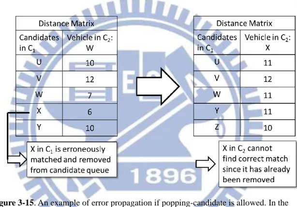
Figure 3-15. An example of error propagation if popping-candidate is allowed. In the
beginning vehicle W is detected in C2 and erroneous matched vehicle X in
C1. Next vehicle X is detected in C2, but X has already been removed from
candidates thus cannot obtain correct result. ... 36
Figure 3-16. Example of the OR. The order of vehicle B and E changed, the S2DP algorithm can only assign one of them. The OR can re-assign B and E. .. 38
Figure 4-1. Five surveillance videos in Hsuehshan tunnel, Taiwan. ... 40 Figure 4-2. Examples of HSTunnel and HSTunnel_NO_MISS. The X symbol
represents miss detection. If one vehicle is miss-detected in one camera, it is removed from HSTunnel_NO_MISS, for example, vehicle 005. ... 40
Figure 4-3. Average performance on different feature descriptors. ... 43 Figure 4-4. Example of an assignment result on (C1, C2). The first row is the candidate
queue contains detections in camera C1, the second row in the second
camera C2, and the third row is an example of execution result. ... 45
Figure 4-5. Experimental result of vehicle groups matching algorithms on HSTunnel.
The x-axis is the number of vehicles in C2 assigned, and y-axis is the
accuracy. ... 48
Figure 4-6. Experimental result of vehicle groups matching algorithms on
HSTunnel_NO_MISS. The x-axis is the number of vehicles in C2 assigned,
and y-axis is the accuracy. ... 49
Figure 4-7. Average accuracy of multi-camera vehicle groups matching algorithms. 50 Figure 4-8. Example of real-time experiments on HSTunnel. The solid lines represent
number of vehicles in the S2DP and dotted lines for the RT. Assume camera C1 starts at vehicle index i and C2 at j. ... 51
ix
Figure 4-9. An example of distance matrix. Most distance values are greater than those
matched ones. ... 57
Figure 4-10. Experiments on miss-match penalty 𝜖 of two datasets. The x-axis is the
value of penalty, the y-axis is corresponding accuracy. ... 58
Figure 4-11. Examples of datasets HSTunnel2 and BGTunnel... 60 Figure 4-12. Overall performance of all methods in datasets HSTunnel, HSTunnel2,
and BGTunnel. The x-axis is the datasets and the y-axis is the average accuracy. ... 62
x
List of Tables
Table 4-1. Properties of dataset HSTunnel. ... 41
Table 4-2. Average performance on CMC values of different feature descriptors. ... 43
Table 4-3. Experimental settings of the real-time methods. ... 51
Table 4-4. Average accuracy of real-time methods on HSTunnel. ... 53
Table 4-5. Average accuracy of real-time methods on HSTunnel_NO_MISS. ... 54
Table 4-6. Comparison of average accuracy using different offline methods. ... 56
Table 4-7. Comparison on the average-distance strategy and the best case of miss-match penalty 𝜖 on HSTunnel. ... 59
Table 4-8. Comparison on the average-distance strategy and the best case of miss-match penalty 𝜖 on HSTunnel_NO_MISS. ... 60
1
Chapter 1. Introduction
In recent years, video cameras are equipped everywhere in our daily life due to the affordable price and easy installation of devices. People can record a mass amount of events passing though the scene by storing the data within videos. However, most of videos contain a lot of redundancies. What we care about is only very small subsets or portions of the videos with semantic meanings. For example, in a traffic surveillance system, what we are interested in is the traffic density of a road section [1] or whether an incident happened [2], and then we can select other path to avoid those sections. For cameras set on streets, we would like to know how many pedestrians passed [3] or if there is any unusual activity [4]; in our living room, system may send alarms if elderly people fall on floor or some dangerous events occur [5]. Therefore, methods to retrieve and summarize useful data efficiently are essential for handling the huge amount of videos.
Research topics on surveillance systems have been discussed in the last decades, for example, object detection, tracking and identification, scene understanding, and event detection [6] [7] [8] [9]. Although different applications are developed for different scenarios, many basic techniques can be applied to most of the surveillance videos. Object detection is usually the first step of a surveillance system to locate the region of interests (ROI), precisely, the object within a scene. After a sequence of video frames is processed, we need to know whether two detected objects from two frames are the same one. This is called object identification or object tracking. Trajectories and paths of detected objects are collected after tracking objects in a period of time. We can use the information to retrieve high-level semantics, such as
2
the number of vehicles passed by and events, car accidents for example.
A traffic surveillance system can reveal various kinds of information. We can monitor the traffic condition by analyzing the videos collected from cameras installed along roads and highways. Intuitively, traffic data like the level of driving speed or the number of vehicles passing by can be provided to drivers or used in navigation systems to avoid congestion areas. Another type of information is whether a specific event happens, like traffic accidents or traffic rule violation. The police nearby can receive alarms from the control center and come to the location quickly. For long-time monitoring, traffic data are stored in databases and we can discuss issues on a road section about congestion or retrieve historic records about some specific vehicles driven by criminals.
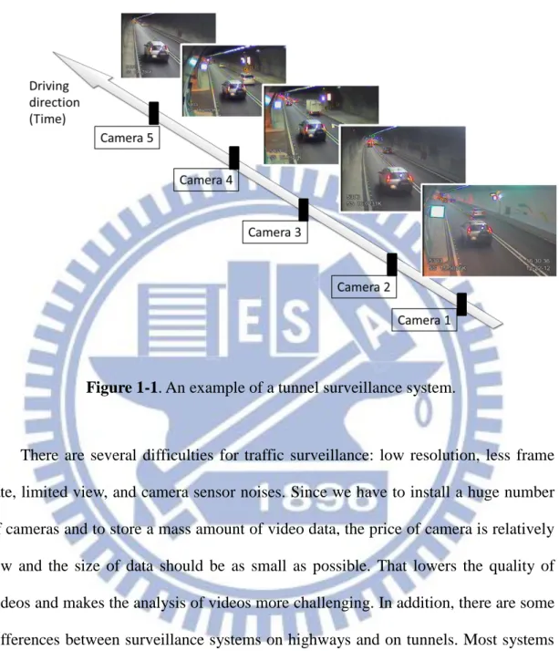
In recent years, researchers focus on tunnel surveillance since accidents in a tunnel may cause serious problems [10]. The traffic agency monitors the traffic condition of a tunnel using multiple surveillance cameras and tries to discover unusual events in real-time. However, that is not an easy task since in most of time monitoring is nothing interesting and makes workers hard to concentrate on the screens. Another shortcoming is that sometimes there are not enough cameras to cover the whole tunnel scene. There are temporal and spatial gaps between videos. Therefore, it is necessary to develop a computer system that can automatically provide precise and brief information. Figure 1-1 shows an example of a tunnel surveillance system that contains multiple cameras. Many surveillance systems on day-time traffic can be directly applied to tunnels because major features are the same as in tunnels. However, more challenges such as poor illumination conditions are present. It is worth considering more aspects on tunnels than on day-time traffic to achieve better
3
performance.
Figure 1-1. An example of a tunnel surveillance system.
There are several difficulties for traffic surveillance: low resolution, less frame rate, limited view, and camera sensor noises. Since we have to install a huge number of cameras and to store a mass amount of video data, the price of camera is relatively low and the size of data should be as small as possible. That lowers the quality of videos and makes the analysis of videos more challenging. In addition, there are some differences between surveillance systems on highways and on tunnels. Most systems on road can only work in day-time. In this case, many basic algorithms can be applied due to sufficient light. However, illumination effects usually exist in tunnels, producing more noise and unpredictable troubles. Fortunately, there are still some benefits in the environments of tunnels, like fewer lanes, more strict driving constraints, and the 24-hour system with the same lighting condition.
4
Another issue is that many traffic surveillance systems do not consider about information between two or more cameras. As a car is driven on a road through multiple cameras, we would first like to know whether two vehicles in two videos are the same. This task is called multi-camera object tracking or multi-camera object identification. It is more challenging than tracking in a single camera, because the view points, poses and lightings are different. These differences may make the visual appearances of an object different in different cameras. Sometimes we cannot track a vehicle across cameras because there are time and space gaps in between. However, we can still identify them by considering the features of each vehicle. A naïve method to identify vehicles between cameras is obtaining the unique license plate number using license plate recognition. However, it is usually not available in a surveillance system due to the poor quality of videos. Hence the robust image features are needed for multi-camera object identification.
In this thesis, we propose a multi-camera vehicle identification system in tunnels. First vehicle detection and tracking are performed in single tunnel surveillance video usingHaar-feature-based cascade detector [11]. After images of vehicles are collected from videos, the visual features of images are then extracted. Features such as color histograms, Haar-like feature vector, SIFT-based feature points and template matching in pixel domain are studied and evaluated by experiments. Next we propose a multi-camera vehicle identification method to identify vehicles between two non-overlapping views of different cameras using calculated feature vectors. The first step is the Spatiotemporal Successive Dynamic Programming (S2DP) algorithm that matches vehicles in two cameras. And then two different algorithms for real-time tracking and offline refinement are proposed for different requirements: the Real-Time (RT) and the Offline Refinement (OR) algorithms following S2DP,
5
respectively. Finally the experiments and discussions on proposed methods are presented in this thesis.
The remaining of this thesis is organized as follows. In Chapter 2, we introduce the related work about surveillance video analysis. Chapter 3 describes the proposed tunnel surveillance system and the multi-camera vehicle identification methods. The experiment settings and experimental results are presented and discussed in Chapter 4. Finally, conclusions and discussions of future work are in Chapter 5.
6
Chapter 2. Related Work
In this chapter, we review the related literatures of video surveillance systems. A survey on methods of object detection, tracking, and multi-camera object identification is presented.
2.1 Video Surveillance Systems
Video surveillance systems are widely used nowadays since cameras are installed everywhere. Applications can be briefly divided by their operating environments, like in-door or out-door and for vehicles or pedestrians. Nevertheless most systems share similar characteristics and require common techniques.
Excellent video processing and computer vision techniques are necessary for a video surveillance system. Researchers try to retrieve useful information and understand the semantics from videos since it is intuitive for human obtaining information from what we see. Buch et al. [12] review the state-of-the-art computer vision techniques for urban traffic system. The common challenges include poor quality of data, wide range of operational conditions and environments, and real-time processing. Key techniques to establish a video-based traffic system are foreground segmentation, shadow removal, feature selection, object classification, and tracking, which are common research topics in computer vision. Zhang et al. [13] survey recent research on data-driven intelligent transportation systems (ITS). The main components of data are from videos, because people are more familiar with visual information. Applications like vehicles or pedestrian detection and tracking, behavior
7
analysis, incident detection, density estimation are discussed often. And systems can be extended by mixing data from different sensors like global positioning system (GPS), laser or infrared radars.
A traffic surveillance system can provide not only real-time processing like vehicle tracking or event detection, but also offline analysis, traffic condition investigation or database indexing for example. Feris et al. [6] propose a system for large-scale indexing of vehicles in a video surveillance system. The idea is providing a database of vehicles in urban environment, with semantic attributes like time, color, size, etc. This can help police easily search for suspicious vehicles and reduce efforts in criminal investigation process. They use some easy but strict constraints to automatically collect and generate a large amount of training patches for vehicle detectors of Haar-based features. Then attributes like time, color, driving direction, color, size, speed, are retrieved for each detected vehicles, and the information is stored into a database.
Sometimes we would like to know the semantic of a scene instead of a specific object, which leads to the topic of scene understanding. For example, the system can automatically discover the moving directions of crowds [8], or the driving paths of vehicles in a scene [14]. The trajectories and motion flows of moving objects can provide features of regular activities. Hence we can discover unusual events by analyzing outliers and anomalies. Atev et al. [14] and Morris and Trivedi [7] try to model the driving behaviors of a road scene in a surveillance video. Since a vast amount of cameras have already been set on road sections and activities might change often, it is necessary to develop an unsupervised way to build the model automatically. By collecting the trajectories of vehicles passing through the scene, both methods
8
apply clustering algorithms and treat each cluster as a usual activity. Morris and Trivedi [7] then train a Hidden Markov Model (HMM) for each activity that can be used as a trajectory classifier. Finally when a new trajectory is obtained, its distance to each cluster can be calculated and abnormal events can be detected. In another aspect, the normal behavior of a road scene can help object detection and tracking. Additional information could assist to predict where the object might be and where it would possibly move to.
2.2 Object Detection and Tracking
A surveillance video contains both specific objects that we are interested in and other unrelated regions, and therefore object detection is usually the first step in a system. As objects are detected in each frame, we need to know whether two detections from two consecutive frames belong to the same object. This requires tracking of each object. Usually both steps are required in a video surveillance system to provide information for further processing.
2.2.1 Object Detection
Sometimes the objects might move, and background subtraction [15] [16] [17] can be applied to videos to obtain those moving objects. Still there are some object detection algorithms in image processing domain like face detection [11] and pedestrian detection [18] techniques, which can also be applied to surveillance video [9] [19] .
9
Background subtraction is a scheme to detect moving objects in videos from static cameras [15], which computes the difference between current frame and a background model, considering the idea that an object is likely different from the background. This is widely applied to surveillance systems since cameras usually are static, and the computation cost is relatively lower than object detection methods. The commonly used approaches include running Gaussian average [20] and Mixture of Gaussians (MoG) [17], which consider the background model as a normal distribution or a mixture of them in pixel domain and detecting foreground object if it is different from the distribution. Brutzer et al. [16] evaluate commonly used and state-of-the-art background subtraction algorithms. The testing scenarios contain dynamic background, darkening, light switch, noise, shadow, and recommended some state-of-the-art algorithms. However, they also state that most background subtraction methods would fail in conditions like noisy night and sudden lighting change, which are quite common in tunnel environments.
Another approach is appearance-based object detection, where the desired objects share common characteristics in an image. Examples include Haar-like feature with cascade classifier [11] and Histogram of Oriented Gradient (HoG) [18], which are widely used in video surveillance systems [6] [10] [19]. Unlike background subtraction methods that usually consider the changes between frames, appearance-based methods treat a video as individual images, not related to neighbor frames. They often require a training step to obtain the common property between objects, and then use sliding window approach to scan the frame and verify whether the region is an object. Appearance-based object detection often needs more computation cost since it requires exhaustive search on the image, but the accuracy is better because it can only find objects similar to the training set.
10
2.2.2 Object Tracking
Object tracking is to figure out where the object is in a video, and the sequence of tracking results can be arranged into a trajectory that presents the history of the movement. An intuitive way is to group detections from two consecutive frames that are in nearby locations. However, there might be noises around the observation. Hence Bayesian tracking [21] can be applied to tracking process. By applying probability formulation, we can track objects more precisely. The common solutions for Bayesian tracking are Kalman Filter and Particle Filter, which constantly update the tracker by taking new observations. Breitenstein et al. [19] propose a multi-person tracking framework using Particle Filter. It is very challenging for object tracking using simple grouping methods in a complex environment because detection cannot perform well. Therefore, filters are necessary in this case. The confidence of detected objects is considered for detections and this solves data association for multi-person tracking.
2.3 Multi-Camera Object Identification and Tracking
An area usually contains multiple surveillance cameras, and it is necessary to mix data from two or more places to obtain more complex information. However, multiple camera processing is far more difficult than single camera processing. For example, lighting, viewpoints, and background in two cameras can be different. Wang [22] reviews recent researches in multi-camera video surveillance. Key technologies in multi-camera systems are multi-camera calibration, computing topology of camera network, tracking, re-identification, and activity analysis. All of them face challenges
11
including various configurations, limited topology, large changes of viewpoints, and illumination conditions. Some of the technologies can be jointly solved. Just as in this thesis, we try to solve the object re-identification problem to achieve multi-camera tracking.
When tracking an object across non-overlapping views of two cameras, two major problems should be solved. Information may not be continuous because there are time and space gaps between two cameras, and the visual appearance changes due to different view angle and lighting of different cameras. Lian et al. [23] propose a method of tracking pedestrians across two cameras using only visual appearance. They calculate the CI-DLBP, the enhanced distance-based local binary pattern (LBP) features that include color information, for each pedestrian. And then match pedestrians from two cameras using the feature vectors to achieve multi-camera tracking. Instead of considering only LBP that describes structural information, color is also an important feature for matching objects from different camera views. They encode a detection of a pedestrian to a histogram of LBP in color space and match two histograms from two different cameras using Chi-square distance, and apply cumulative brightness transfer function (CBTF) to reduce the illumination effect in pre-processing steps.
Cabrera et al. [9] propose a method of multi-camera vehicle tracking-by-identification in a tunnel surveillance system. Like [6], they use Haar-like feature to detect vehicles in a single camera and obtain a feature vector with binary values of weak classifiers for all detections. Next they use Hamming distance to find the best matched pairs for each vehicle in both single camera tracking and multi-camera identification. The two major advantages of this method are: the
12
computation of Haar-like features can be efficiently obtained, and the lower cost in passing and comparing feature vectors with binary values. The authors state that color is not reliable in tunnels because it may be affected by lighting. However we think that color is still a strong feature for vehicles especially when the resolution is quite low in surveillance video. Some practical issues have not been discussed, such as system initialization and error handling, which is presented in this thesis.
13
Chapter 3. Multi-Camera Vehicle Identification
In this chapter, we illustrate the multi-camera vehicle identification framework in detail. An overview will be given in Section 3.1 and single-camera vehicle detection and tracking is described in Section 3.2. Next, possible image features for identification is presented in Section 3.3. The proposed multi-camera vehicle identification method and the real-time and offline identification are illustrated in Section 3.4 and 3.5, respectively.
3.1 An Overview of the Proposed Framework
Figure 3-1 shows the framework of the proposed system. Starting from a single camera, we first extract vehicles passing through the scene by object detection and tracking. After a period of time we can collect a set of vehicle patches. The number of detected vehicles in the first camera is always more than the number in the next camera, since there are vehicles passing the first camera but not the second one. In other words, when a vehicle is presented in the second camera, multi-camera tracking/identification is to search for the corresponding detection in the first camera that represents the same vehicle.
14
Figure 3-1. System framework.
In a single camera, all passing vehicles are discovered using Haar-like feature detector [11] for each frame. And within a small interval of a video sequence, vehicles are tracked by considering the location in the image of detections from consecutive video frames. As vehicles in tunnel travel in sequence, we can use a queue to store all tracked vehicles to preserve the order. Single-camera vehicle detection and tracking will be discussed in Section 3.2 in detail and a dataset of the detection results with five cameras are presented in Section 4.1.
For object recognition and identification, we extract features from the object images. Color and visual structure information are important features for vehicle identification in a low resolution surveillance video. Section 3.3 discusses some commonly used feature descriptors that encode the visual features, and Section 4.2 evaluates these descriptors.
15
After a period of time, we can collect a set of queues with detected vehicles from several cameras in the same tunnel. We need to initialize the system first to verify which vehicle is the first one that exists in all queues. Because there may be vehicles between two cameras, and when we start recording multiple cameras at the same time, there may be vehicles in latter cameras that do not appear in the previous ones. One solution is to start recording multiple cameras in different time, however it is still hard to correctly make one vehicle become the first entity in all detection queues, unless there is no vehicle in the tunnel. We accomplish the task by considering the ordering constraint within a tunnel. That is, one vehicle is behind another most of the time and the order rarely changes, as well as lane changing is often prohibited in a tunnel. Therefore, a multi-camera identification method is proposed based on the ordering constraints of vehicles. In the beginning the Spatiotemporal Successive Dynamic Programming (S2DP) algorithm matches vehicles from two cameras. Next, the Real-Time (RT) algorithm can be applied after S2DP for real-time vehicle tracking, and the Offline Refinement (OR) algorithm can further achieve higher accuracy from the results of S2DP.
The S2DP algorithm matches vehicles in two detection queues, and thus achieves multi-camera identification. However, it has to check a group of detections at the same time and cannot run in real-time. The RT can accomplish the identification task in real-time, picking up the most similar one in a small search window of the detection queue. Nevertheless, real-time algorithm usually shows lower accuracy, and is sometimes not suitable for database applications, which do not require real-time processing but the accuracy need to be assured. In this case we propose another offline identification method, OR, which is used to achieve higher accuracy by refining the results from S2DP. The real-time and offline algorithms are discussed in
16
Section 3.5 and experiments are presented in Section 4.4.
3.2 Vehicle Detection and Tracking in Single Camera
The first step of the system is to obtain information from cameras independently, thus we will discuss single-camera vehicle detection and tracking method in this section. We use Haar-like feature detector [11], which is commonly used in face detection, to detect vehicles in a tunnel surveillance video. And the same method is used in [6] and [10] for vehicle detection. For a sequence of detections from consecutive video frames, we group them by considering the location of detections in x-y coordinate of frames to achieve vehicle tracking.
3.2.1 Vehicle Detection
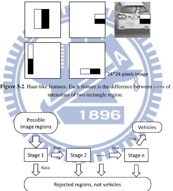
We use Haar-like feature detector [11] to detect vehicles in a video frame. The Haar-like features are a set of binary values which consists of the differences between two or more sums of intensities in rectangle regions of a grayscale image, as shown in Figure 3.2. Since there are various sizes of rectangles, a 24*24 resolution image, which is the size of our training images, can obtain a great amount of features in the exhaustive set of rectangle regions. As the visual structures of vehicles are similar in surveillance videos, vehicles share the same subset of Haar-like features, which do not appear in other regions of the videos. Therefore, we can discover those shared Haar-like features by applying machine learning algorithms and obtain a vehicle detector/classifier for videos. The learning algorithm uses a cascade of Adaboost classifiers to choose proper weak classifiers, the Haar-like features, and forms a stronger classifier. The cascade consists of a number of stages that reject negative
17
examples. Finally if an image passing all cascading stages, the detector will classify it as positive detection. Figure 3.3 illustrates the cascading scheme. The method uses integral images to fast calculate features, considers only a small subset of all possible Haar-like features, and rejects negatives in a short time by cascading stages. As the result, the algorithm can be used in real-time detection.
Figure 3-2. Haar-like features. Each feature is the difference between sums of
intensities of two rectangle region.
Figure 3-3. The cascading scheme of Haar-like feature detector.
The traditional method for object detection in surveillance video is background subtraction, because the objects usually move in the video. In fact, the vehicles always
18
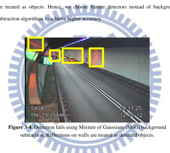
move on the roads. However, reflections of headlights and taillights often exist on the wall of tunnels and those reflection regions might be treated as foreground objects in background subtraction methods. Another problem is that one vehicle may be occluded by another vehicle such that the algorithm may produce one big object instead of two. Figure 3-4 shows an example of problems in background subtraction using Mixture of Gaussians (MoG) [17] method, where the light reflections on walls are treated as objects. Hence, we choose feature detectors instead of background subtraction algorithms to achieve higher accuracy.
Figure 3-4. Detection fails using Mixture of Gaussians (MoG) background
subtraction. Reflections on walls are treated as detected objects.
3.2.2 Vehicle Tracking
The goal of vehicle tracking is to find the corresponding detections of the same vehicle in different frames. Detection contains the image features, coordinates of the bounding box in image, detected time, and other related properties. We can keep track of detections which have similar properties. That is, if two detections from two consecutive frames have similar properties, these two detections present the same
19
vehicle. Since the detection is not accurate all the time and contains noise, it is common to apply Kalman Filter or Particle Filter [21] to predict the actual state of the object.
As vehicles always drive forward in tunnels, we simply take the coordinates of detections in an image as the properties for tracking. If two detections from two frames are in similar location within the image, we treat them as a single object. After one object is tracked in five consecutive frames, where the frames per second (FPS) of our video is about 10 and the vehicle is around the middle position of the video, the image of this object in the fifth frame is stored into the detection queue of the camera. Each camera maintains a queue of tracked vehicles, so that the ordering of passing vehicles can be recorded. The tracking step can also help us remove wrong detections because noises usually do not move. Every image stored in detection queue is resized to 40*40 pixels for further processing.
3.3 Feature Extraction
As we obtain a vehicle from one camera, we need to transfer the image patch into a feature vector that is proper for object identification. The goal is to select the best feature that can clearly identify whether two detections from two different cameras belong to the same one or not using distance metric. In this section we will introduce four possible feature descriptors for our multi-camera identification application. Experiments will be presented in Section 4.2.
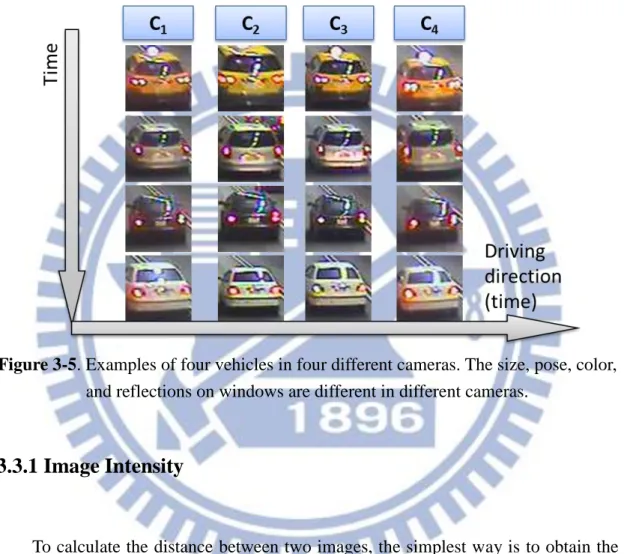
The feature should minimize the effects on visual appearances in multi-camera identification: poses, color, illumination and noises. Figure 3-5 illustrates these
20
challenges. Another problem is that the images are in small resolution such that the details of a vehicle are hard to describe by features. Nevertheless we can take advantage of shorter computation time. In conclusion we choose Harris corner detection with OpponentSIFT [24] as our selected feature.
Figure 3-5. Examples of four vehicles in four different cameras. The size, pose, color,
and reflections on windows are different in different cameras.
3.3.1 Image Intensity
To calculate the distance between two images, the simplest way is to obtain the sum of squared difference (SSD) of intensities between every pixel in them. In our application, the resolution of our detected vehicle is 40*40 for all images and the distance can be calculated in one pass for each color channel. Consider the application in RGB color space, and the image intensities (int) distance between two images 𝐼1 and 𝐼2 is
𝑑𝑖𝑛𝑡(𝐼1, 𝐼2) = ∑ ∑(𝐼1(𝑥, 𝑦) − 𝐼2(𝑥, 𝑦))2 𝑥,𝑦
21
where 𝐼𝑖(𝑥, 𝑦) is the intensity of image 𝑖 at (𝑥, 𝑦), and sum the values of all RGB channels.
3.3.2 Color Histograms
Histograms describe the distribution of intensities for an image. Here we tested histograms in three different color spaces: RGB, hue, and opponent color space. RGB histogram is a basic way to describe an image, since the input image is in RGB color space. Because color is one of the important features of vehicles, another selected color space is hue which describes the color distribution of an image. Hue is converted from RGB by
𝐻𝑢𝑒 = {
60(𝐺 − 𝐵)/(𝑚𝑎𝑥(𝑅, 𝐺, 𝐵) − 𝑚𝑖𝑛(𝑅, 𝐺, 𝐵)) 𝑖𝑓 𝑚𝑎𝑥(𝑅, 𝐺, 𝐵) = 𝑅 120 + 60(𝐵 − 𝑅)/(𝑚𝑎𝑥(𝑅, 𝐺, 𝐵) − 𝑚𝑖𝑛(𝑅, 𝐺, 𝐵)) 𝑖𝑓 𝑚𝑎𝑥(𝑅, 𝐺, 𝐵) = 𝐺 240 + 60(𝑅 − 𝐺)/(𝑚𝑎𝑥(𝑅, 𝐺, 𝐵) − 𝑚𝑖𝑛(𝑅, 𝐺, 𝐵)) 𝑖𝑓 𝑚𝑎𝑥(𝑅, 𝐺, 𝐵) = 𝐵 Finally we choose histograms in opponent color space. The color space consists of three channels, the first two channels represent relation between RGB information and the third channel represents the grayscale intensity. Opponent color space can be converted from RGB using
( 𝑂1 𝑂2 𝑂3) = ( (𝑅 − 𝐺)/√2 (𝑅 + 𝐺 − 2𝐵)/√6 (𝑅 + 𝐺 + 𝐵)/√3 )
For every histogram, we extract 64 bins for each channel, therefore the RGB and opponent histogram has 192 bins and hue histogram has 64 bins. The distance between two histograms is the Chi-square distance
𝑑𝐶𝐻(𝐻1, 𝐻2) = ∑(𝐻1(𝑗) − 𝐻2(𝑗))
2
𝐻1(𝑗)
𝑗
22
3.3.3 Haar-Like Feature Vector
Haar-like feature vector is obtained from the vehicle detector. It is a set of binary values with 143 dimensions, where we have 143 selected features in our trained detector. Cabrera et al. [10] stated that this feature can be used in multi-camera identification, without additional steps of feature calculation. Figure 3-2 shows an example of the feature. Hamming distance is used as distance metric since the feature vector contains only binary values, and the same vehicle would have similar result in the vector. The Hamming distance is computed by
𝑑𝐻𝑉(𝑇1, 𝑇2) = ∑|𝑇1(𝑗) − 𝑇2(𝑗)| 𝑗
where 𝑇𝑖 is the binary vector of image 𝑖, and 𝑇𝑖(𝑗) is the value of the 𝑗th element.
3.3.4 Keypoints Descriptors
Keypoints descriptors are commonly used in object recognition.Generally, some points in an image contain rich information. Those points are called keypoints, interesting points, or corners. Keypoints are extracted from the image, and then each point is represented with a specific descriptor. One of the famous keypoint extraction methods is Scale-Invariant Feature Transform (SIFT) [25], which is a powerful tool in many computer vision applications. SIFT finds keypoints using Difference-of-Gaussians (DoG) and describes each point using a histogram with orientation information around that point. The method can achieve high accuracy but the computation speed is relatively low if the image is large. Our selected keypoints descriptors are SIFT, ORB [26], and Harris corner detection with OpponentSIFT descriptor [24]. Figure 3-6 illustrates the keypoints descriptor algorithms.
23
Figure 3-6. A general illustration of keypoints descriptors.
Oriented BRIEF (ORB) [26] tries to reduce the computation time while not reducing much of accuracy compared with SIFT. The algorithm starts by detecting FAST [27] keypoints in an image, which considers the intensity differences between one center pixel and its neighbors in a circular ring. Next ORB uses BRIEF [28] descriptors to encode each detected keypoint into a bit string. The orientation and rotation properties of an image are considered in both keypoint detection and description processes. The whole processing time is much faster than SIFT, since both keypoints detection and description methods are simpler. However, the performance is not as superior as SIFT.
Van de Sande et al. [24] evaluate different features for object recognition. They analyze the invariant properties of different color descriptors, histograms, moments, and SIFT descriptors, with test on public datasets. The authors state that OpponentSIFT, which computes SIFT descriptor in opponent color space, is recommended since it outperforms other descriptors and is invariant to light intensity changes and shifts. Although our application is a little bit different from the
24
experiments in their work, Section 4.2 shows similar result that OpponentSIFT has higher accuracy than other methods described in this section. In their detection process they use Harris-Laplace corner detector to obtain more accurate points without unnecessary points. Since our input image is far smaller and the object is located in the center, we use only Harris corner to reduce computation time.
For all keypoint descriptors, we compute the Euclidean distance between feature vectors of two images 𝐼1 and 𝐼2. First, we extract 10 keypoints, which are enough for our detected images with size of 40*40 pixels, in each image. And the feature vector is obtained using descriptors introduced before. For each point, SIFT descriptor is a vector of integers with 128 dimensions of orientation histogram, where ORB has 256 dimensions and OpponentSIFT has 3*128 dimensions of three channels in opponent color space. Next we use brute-force method to assign a corresponding point in 𝐼2 with smallest Euclidean distance for a point in 𝐼1. Therefore, we can obtain 10 distance values since there are 10 keypoints in an image, and one point in 𝐼2 may have chance being assigned more than once. For 𝐼2, we again use the same method to obtain 10 distance values corresponding to 𝐼1. Finally the distance between the two images is the average value of the 20 distance values. The method can be formulated as 𝑑𝐾𝐷(𝑃𝐼1, 𝑃𝐼2) = 1 2( (∑ min 𝑗 𝑑𝑖𝑠𝑡(𝑃𝑖 𝐼1, 𝑃 𝑗𝐼2) 𝑖 ) |𝑃𝐼1| + (∑ 𝑚𝑖𝑛 𝑖 𝑑𝑖𝑠𝑡(𝑃𝑗 𝐼2, 𝑃 𝑖𝐼1) 𝑗 ) |𝑃𝐼2| )
where 𝑃𝑖𝐼1 is the 𝑖th keypoint descriptor of image 𝐼1 and 𝑃𝑗𝐼2 is the 𝑗th keypoint descriptor of image 𝐼2. 𝑃𝐼1 = {𝑃
1𝐼1, … , 𝑃𝑛𝐼1} and 𝑃𝐼2 = {𝑃1𝐼2, … , 𝑃𝑚𝐼2} is the set of
keypoint descriptors of 𝐼1 and 𝐼2, respectively. The |∙| represents the number of elements in a set. The 𝑑𝑖𝑠𝑡(𝑃𝑖𝐼1, 𝑃𝑗𝐼2) is the distance between 𝑃𝑖𝐼1 and 𝑃𝑗𝐼2. Note that
25
the Euclidean distance is applied on SIFT and OpponentSIFT descriptors, and Hamming distance is for ORB descriptors.
As our experimental result in Section 4.2, OpponentSIFT outperforms other features and is selected for further processing.
3.4 Multi-Camera Vehicle Groups Matching
This section illustrates the problem of multi-camera vehicle identification and describes the proposed algorithms for tunnel application. We collect vehicles from cameras as described in Section 3.2, and compute the feature vector for each vehicle in Section 3.3. Each camera maintains a queue of detected vehicles with computed feature vectors. Now, we can identify vehicles from different camera by matching feature vectors in two queues. This is called multi-camera identification, object re-identification [22], object matching [23], or multi-camera tracking-by-identification [9].
For each camera, we keep a queue of detected vehicle patches ordered by time. Different cameras are also ordered by time since they are set on road that vehicles must pass in order. If we focus on only two cameras, the identification is reduced to an assignment problem. That is, finding all matched pairs of vehicles from two queues with the smallest sum of distances, and every vehicle can be assigned only once. In Figure 3-7, assume that we have to assign three vehicles from camera C1 and C2. First
we can compute the distance matrix using feature vectors described before, and then apply greedy method or some well-known solutions such as Hungarian algorithm [29] to find matching pairs of vehicles.
26
Figure 3-7. Assignment problem in multi-camera vehicle identification.
The major difficulties are the problems in appearance changing of the same vehicle in different cameras, which would be solved by using OpponentSIFT. However, vehicles may look similar or are of the same type that exists in the tunnel within a small period of time. Matching vehicles using only appearance information may have errors sometimes. In other words, matching pairs of vehicles using only the distance matrix obtained by visual features, Figure 3-7 for example, cannot achieve suitable performance, especially when the distance matrix is quite large. Besides, there is a time gap between two cameras, so we can only roughly guess when a vehicle might pass the second camera. This requires a certain number of vehicles to be considered at the same time since we cannot know the exact time a vehicle passed by.
3.4.1 Spatiotemporal Successive Dynamic Programming (S
2DP)
The Spatiotemporal Successive Dynamic Programming (S2DP) algorithm is proposed to solve the identification problem in tunnels by considering the ordering
27
constraint. Given a distance matrix of detected vehicles in two cameras, the S2DP finds one vehicle from the first camera for each vehicle in the second camera.
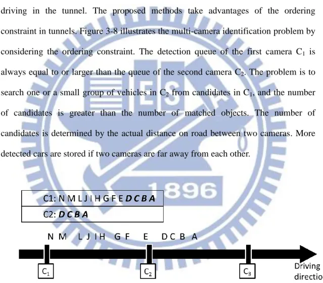
Ordering constraint [30] exists in road that all vehicles are in some kinds of successive sequence, especially when lane changing is prohibited in long tunnels for traffic safety. More specifically, a car is possibly behind another one during the whole driving in the tunnel. The proposed methods take advantages of the ordering constraint in tunnels. Figure 3-8 illustrates the multi-camera identification problem by considering the ordering constraint. The detection queue of the first camera C1 is
always equal to or larger than the queue of the second camera C2. The problem is to
search one or a small group of vehicles in C2 from candidates in C1, and the number
of candidates is greater than the number of matched objects. The number of candidates is determined by the actual distance on road between two cameras. More detected cars are stored if two cameras are far away from each other.
Figure 3-8. An example scenario on multi-camera vehicle identification. Assume each
capital letter represents an individual vehicle.
In the beginning, we are not sure where the exact position of the desired candidate is in the queue, so we need to search in a window of proper size and position, with respect to the detection queue of previous camera. The size of the
28
window is important since the more the candidates are included, the more the noises are contained, which affects the performance. Therefore, the first thing to do is to find the proper location of the search window in the queue of first camera, and then we will have the ability to minimize the size of the window. We call this step as an initialization problem. As illustrated in Figure 3-8, the first vehicle A need to be correctly identified, thus vehicle B can be easily found by considering the ordering constraint. If, unfortunately, vehicle A in camera C2 is matched to vehicle H in camera
C1, then vehicle B in C2 can never find a correct matching since B is not behind H.
Therefore, the initialization problem is an important issue when the ordering of objects is taken into account.
It is worth noting that not all vehicles in the second camera can find a corresponding detection in the first camera, and vice versa. Because the vehicle detection cannot certainly reach 100% of accuracy, there are always miss detections in all cameras. In addition, when each camera passes information to the central server using the Internet, there may have packet losses or disconnections sometimes that implicitly yield miss detections. Consequently the algorithm must incorporate the miss detection problem.
Since the ordering constraint is an important characteristic and the miss detection problem needs to be considered, we propose a dynamic programming algorithm S2DP to solve the assignment problem. Assume that we have a 𝑁1𝐶× 𝑁2𝑐 distance matrix 𝐷 where the two axes contain 𝑁1𝐶 and 𝑁
2𝐶 vehicles in camera 𝐶1 and 𝐶2,
respectively. 𝐷(𝑖, 𝑗) = 𝑑𝐾𝐷(𝑃𝐼𝑖, 𝑃𝐼𝑗) is the distance between two feature vectors of
vehicle 1 ≤ 𝑖 ≤ 𝑁1𝐶 in 𝐶1 and vehicle 1 ≤ 𝑗 ≤ 𝑁2𝐶 in 𝐶2 using keypoints descriptor described in Section 3.3. The dynamic programming cost function 𝑓 is
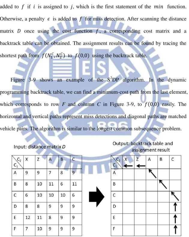
29 defined as 𝑓(𝑖, 𝑗) = 𝑚𝑖𝑛 { 𝑓(𝑖 − 1, 𝑗 − 1) + 𝐷(𝑖, 𝑗) + 𝜆 ∗ 𝑠𝑡𝑒𝑝 𝑓(𝑖 − 1, 𝑗) + 𝜖 𝑓(𝑖, 𝑗 − 1) + 𝜖
where 𝜖 is the miss-match penalty, 𝜆 is the Non-Spatiotemporal-Successiveness (NS2) penalty, and 𝑠𝑡𝑒𝑝 is the number of steps from the last assignment. 𝐷(𝑖, 𝑗) is added to 𝑓 if 𝑖 is assigned to 𝑗, which is the first statement of the 𝑚𝑖𝑛 function. Otherwise, a penalty 𝜖 is added to 𝑓 for miss detection. After scanning the distance matrix 𝐷 once using the cost function 𝑓 , a corresponding cost matrix and a backtrack table can be obtained. The assignment results can be found by tracing the shortest path from 𝑓(𝑁1𝐶, 𝑁2𝐶) to 𝑓(0,0) using the backtrack table.
Figure 3-9 shows an example of the S2DP algorithm. In the dynamic programming backtrack table, we can find a minimum-cost path from the last element, which corresponds to row F and column C in Figure 3-9, to 𝑓(0,0) easily. The horizontal and vertical paths represent miss detections and diagonal paths are matched vehicle pairs. The algorithm is similar to the longest common subsequence problem.
30
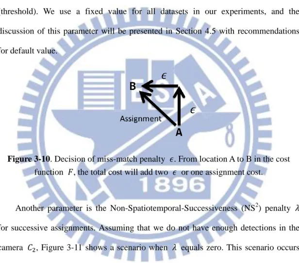
The value of the miss-match penalty 𝜖 is determined by both the distance function 𝑑𝐾𝐷 and the proper threshold to claim miss detections. The total cost 𝑓 will add 𝜖 twice if one assignment is skipped since one element in row and one in column have to be added to move to the same position. As illustrated in Figure 3-10, two 𝜖 or one assignment cost from location A to location B will be added to the cost function 𝑓. Therefore, we set 𝜖 as half of the maximum-allowed matching distance (threshold). We use a fixed value for all datasets in our experiments, and the discussion of this parameter will be presented in Section 4.5 with recommendations for default value.
Figure 3-10. Decision of miss-match penalty 𝜖. From location A to B in the cost
function 𝐹, the total cost will add two 𝜖 or one assignment cost.
Another parameter is the Non-Spatiotemporal-Successiveness (NS2) penalty 𝜆 for successive assignments. Assuming that we do not have enough detections in the camera 𝐶2, Figure 3-11 shows a scenario when 𝜆 equals zero. This scenario occurs when two cameras are far away from each other in the initialization step. The total cost between the solid path and the dotted path are nearly the same, thus we may have chance to choose the dotted one, which is wrong, instead of the solid one when noise is included. If the number of elements in one axis is much less than the other, then the assignment may not be successive since the distance cannot provide enough information due to noise of visual features in the distance matrix. Here, the successive assignment means that assigned elements are next to each other, which satisfies the
31
ordering constraint that vehicles go through the tunnel in order and cannot disappear. Therefore, we select the path that assignments are more successive with the consideration of ordering constraint. For each assignment, we add the NS2 penalty 𝜆 to the distance, multiplied by the number of steps from previous assignment. If the 𝑓(𝑖, 𝑗) is far away from previous assignment, then the penalty is big enough to make miss match as final decision. We define 𝜆 = 𝛼𝜖 that is related to 𝜖 and 𝛼 is the weight. In our experiments 𝛼 = 0.01 is enough to accomplish the task.
Figure 3-11. A scenario without Non-Spatiotemporal-Successiveness (NS2) penalty 𝜆 (dotted path).
3.5 Real-Time and Offline Vehicle Identification
This section describes our real-time and offline identification process. The first step is S2DP presented in Section 3.4. However, two problems show up in the S2DP: cannot run in real-time, and cannot assign order-changed vehicles. We employ two additional algorithms to solve the two problems after the S2DP.
32
First, the S2DP cannot run in real-time since it requires a number of vehicles appear in both camera queues. For example, at least 15 vehicles are required to achieve reasonable accuracy in our experimental result in Section 4.2. Sometimes we would like to identify a vehicle immediately when it appears in the second camera, just like multi-camera vehicle tracking. If the initialization problem is solved by S2DP, we can lower the size of the search window and identify the corresponding vehicle with a small number of candidates in the queue.
Another problem is that, if one vehicle changed its order in two cameras, the S2DP would fail to assign this vehicle. Figure 3-12 shows an example of the situation. Vehicle C is in front of vehicle B in the second camera and B cannot find proper assignment because the ordering constraint does not allow B in C2 to assign the one
prior to C in C1. Hence B in C2 will get a “no-match” result. The problem will occur
in two situations: one vehicle overtakes another one, or multiple driving lanes are in the video and the driving speed of one lane is faster than that of another one. Although in many tunnels overtaking of vehicles is not allowed, there are still vehicles not obeying the traffic rules. And in our dataset, we do not record which driving lane a detected vehicle was to make our work more flexible. Hence the problem is considered in this section. In fact the methods automatically detecting driving lanes in a surveillance video [14] [7] can be applied to our system for better vehicle detection.
33
Figure 3-12. The order of vehicle B and vehicle C in camera C1 are changed in
another camera C2. S2DP algorithm can only assign one of them.
The remaining sections are organized as follows: in Section 3.5.1 we will describe the Real-Time (RT) algorithm for fast assignment of a proper candidates using sliding window approach. If real-time processing is not required, another Offline Refinement (OR) algorithm to solve the problem with higher identification accuracy is presented in Section 3.5.2.
3.5.1 Real-Time Identification
Assume we finish the S2DP algorithm that all vehicles in the second camera are assigned. Then, if a new vehicle shows up in the second camera, we can assign a candidate to this vehicle in real time. Instead of considering a group of vehicles from two cameras in S2DP, the Real-Time (RT) algorithm only takes one vehicle in the latter camera for identification. RT does not have to wait for a number of vehicles passing by, thus achieve real-time processing. This section describes a simple greedy algorithm that achieves real-time processing of the identification problem.
Given the computation result of the S2DP and a feature vector of one newly detected vehicle in the second camera, the RT assigns one candidate vehicle to the newly detected one. As we finish the initialization step using S2DP, a newly detected
34
vehicle in the second camera is possibly next to the last assigned one in the first camera. This property suggests us of using a sliding window approach to solve the problem.
The Real-Time (RT) algorithm runs as follows. First set a search window in the detection queue of the first camera just around the last assigned vehicle in the S2DP, since a newly detected vehicle in latter camera is probably behind it according to the ordering constraint. Considering the example in Figure 3.8, the S2DP matches vehicle A to vehicle D. As vehicle E is detected in camera C2, the desired matching candidate
in C1 is probably around vehicle D. The size of the window is limited to a small value
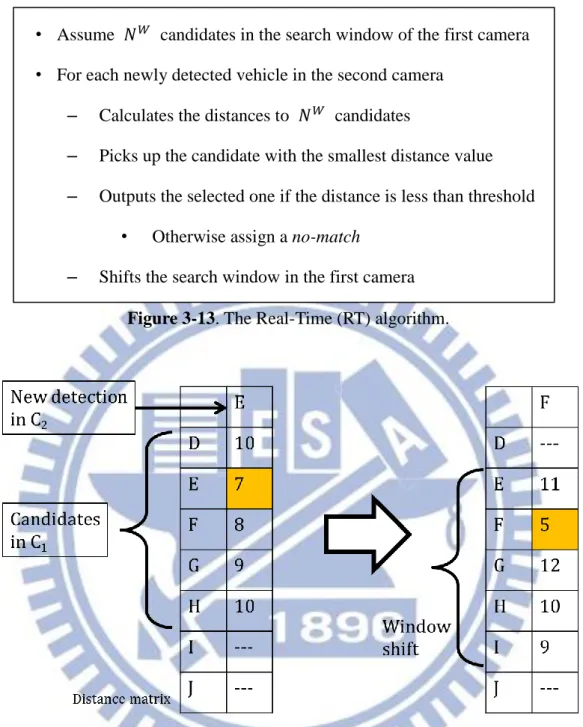
for real-time processing, for example, five vehicles in our experiments. Notice that the detection queue of the first camera always contains unassigned vehicles since it is prior than the second camera. If a vehicle appears in the second camera, we calculate the feature vector of the detection and compute the distance to all vehicles in the search window of the first camera. The one in the first camera with the smallest distance is picked up and treated as the assignment result. If all distance values are greater than the matching threshold, which is greater than 2𝜖 in S2DP, a no-match is assigned. Finally we slide the search window to the next one in the detection queue of the first camera, and this process loops again. Figure 3-13 describes the RT algorithm in detail. As an execution example shown in Figure 3-14, only five candidates in C1
are considered when vehicle E is detected in camera C2. The candidate with smallest
distance is matched. Next five candidates are changed using sliding window approach for the next detected vehicle F in C2. Note that only the candidates in the search
window are taken into consideration. The distance values of others, for example, candidate J, are not computed and are represented using dots.
35
Figure 3-13. The Real-Time (RT) algorithm.
Figure 3-14. An example of RT. Each capital letter represents one vehicle, and the
table is the distance matrix. Only the distance values of candidates are computed and presented using numbers.
The RT algorithm allows one candidate in the first camera being matched to two or more new detections in the second camera. It is strange and erroneous that one vehicle became two in another camera. However in our experiments, we found that error may propagate if we do not enforce the property and produces poor identification results. Consider the scenario in Figure 3-15 that vehicle X in the first
• Assume 𝑁 candidates in the search window of the first camera • For each newly detected vehicle in the second camera
– Calculates the distances to 𝑁 candidates
– Picks up the candidate with the smallest distance value – Outputs the selected one if the distance is less than threshold
• Otherwise assign a no-match
36
camera C1 is assigned to vehicle W in the second camera C2, which is an incorrect
assignment. The algorithm would delete X from the candidate queue if we do not allow re-assignment. Next vehicle X in C2 was detected, however X in the candidate
queue had already been erased and the assignment would certainly incorrect. If X in C2 still got another false assignment, then this error propagated. Therefore an
incorrect assignment will possibly produce at least two errors in the final result.
Figure 3-15. An example of error propagation if popping-candidate is allowed. In the
beginning vehicle W is detected in C2 and erroneous matched vehicle X in C1. Next
vehicle X is detected in C2, but X has already been removed from candidates thus
cannot obtain correct result.
Another characteristic is that the last assignment in the first camera has to be a correct assignment. Otherwise the initial position of the sliding window would be inappropriate and the correct candidate would never appear in the search window. Hence the whole real-time identification results would be wrong. To make sure the algorithm can correctly find the location of the sliding window, we discard the last three results in the S2DP and re-assign them in the RT. Using the S2DP algorithm can
37
make all assigned candidates close to each other by considering the NS2 penalty. However, the vehicles in the end of the matched group cannot be matched correctly since the last few vehicles of the group have too little information to be matched. Consequently, we discard the last three assignments and re-assign them in the RT.
Finally, to enhance the effect of ordering constraint 𝜆 ∗ 𝑠𝑡𝑒𝑝 is added to all distance values, where 𝜆 is the NS2 penalty and 𝑠𝑡𝑒𝑝 is number of steps from previous assignment.
3.5.2 Offline Refinement
The RT algorithm can run in real-time, but the performance is limited because it only considers one vehicle for one assignment. As stated in the S2DP, the ordering constraint is an important feature and we should consider a group of vehicles instead of one. Therefore, we develop another algorithm Offline Refinement (OR) achieve higher accuracy. Another problem is that the S2DP algorithm cannot properly assign order-changed vehicles.
We propose the Offline Refinement (OR) algorithm to solve these problems. We found that order-changed vehicles can be solved using a second pass assignment. Figure 3-16 shows an example that vehicle B and E are order-changed vehicles and cannot be assigned by S2DP. As vehicle B and vehicle E are both missed in camera C1
and C2, we can re-assign the missed vehicles. In fact all order-changed vehicles will
possibly leave un-assigned in S2DP. We can simply apply Hungarian algorithm to the vehicles that are missed in the S2DP. That is, vehicle B and vehicle E in Figure 3-16 are matched using optimal assignment algorithm.
38
Figure 3-16. Example of the OR. The order of vehicle B and E changed, the S2DP algorithm can only assign one of them. The OR can re-assign B and E.
The penalty 𝜆 ∗ 𝑠𝑡𝑒𝑝 is added to each element in the distance matrix, where 𝜆 is NS2 penalty, and 𝑠𝑡𝑒𝑝 is the number of detections between two vehicles, just like in S2DP and RT. Similarly, after applying Hungarian algorithm in the OR, we will check the distance values of each assignment, and report miss detections if the value is greater than threshold 2𝜖, the same threshold value as in S2DP.
39
Chapter 4. Experiments
This chapter presents the experiments on our proposed methods. First, we will introduce the manually labeled datasets for experiments in Section 4.1. Experiments on feature selection, the S2DP multi-camera identification, and real-time and offline methods are presented in Section 4.2, 4.3 and 4.4, respectively. Finally the discussions on the threshold 𝜖 in our algorithm and the performance on other datasets are discussed in Section 4.5.
4.1 Datasets
The surveillance videos from five cameras in Hsuehshan tunnel, Taiwan [31] are collected. Every vehicle drives through five cameras from camera C1 to camera C5
and the driving distance between each camera is one kilometer in average. We manually label 195, 195, 148, 150, 173 vehicles in C1 to C5, respectively, and each
labeled vehicle is a colored image of size 40*40. Assume that all vehicles are presented in C1 and C2, and C3, C4, C5 including miss detections. The detection rate in
each camera is 100%, 100%, 76%, 77%, and 89%, respectively. The numbers of order-changed vehicles in C1 to C5 with respect to C1 is 0, 6, 10, 12, and 19. Here we
call this dataset as HsuehShanTunnel (HSTunnel).
Another dataset HSTunnel_NO_MISS is a subset of HSTunnel. All five cameras contain 124 vehicles respectively, which is the intersection of all cameras in HSTunnel. Assume there is no miss detection in this dataset. The numbers of order-changed vehicles with respect to C1 are 0, 0, 5, 4, and 8 in C1 to C5, respectively.
HSTunnel_NO_MISS can give us the best performance of our experiments since one major issue, miss detection, is removed. Figure 4-1 shows the examples of each