科技部補助專題研究計畫成果報告
期末報告
利差交易報酬之總體經濟因素分析
計 畫 類 別 : 個別型計畫 計 畫 編 號 : MOST 103-2410-H-004-091-執 行 期 間 : 103年08月01日至104年12月31日 執 行 單 位 : 國立政治大學金融系 計 畫 主 持 人 : 林建秀 計畫參與人員: 碩士班研究生-兼任助理人員:謝仲 碩士班研究生-兼任助理人員:謝皓雯 碩士班研究生-兼任助理人員:黃褀真 碩士班研究生-兼任助理人員:歐哲源 處 理 方 式 : 1.公開資訊:本計畫涉及專利或其他智慧財產權,2年後可公開查詢 2.「本研究」是否已有嚴重損及公共利益之發現:否 3.「本報告」是否建議提供政府單位施政參考:否中 華 民 國 105 年 03 月 28 日
中 文 摘 要 : 本計畫探討總體經濟因素透過馬可夫轉換機率而影響到利差交易報 酬的效果。為了衡量利差交易報酬的總體經濟因素之效果,我們採 用隨時間變動之轉換機率的馬可夫狀態轉換模型。我們將幾個總體 經濟變數放 入模型中,衡量哪種變數可解釋利差交易報酬的變化,並期望找出 影響UIP 成立與否之總體經濟變數。我們用馬可夫狀態轉換模型得 到兩種狀態:其中一種捕捉UIP 被違反且利差交易有高報酬的狀態 ;另一種則是UIP 成立且發生貨幣危機的時期。此外透過隨時間變 動之轉換機率的馬可夫狀態轉換模型之估計,我們發現實質匯率可 有效幫助預測市場由高利差報酬時期轉向低利差交易報酬時期,也 將幫助政府和市場參與者藉由實質匯率的變動預測匯率的改變並對 利差投資組合作適當的配置. 中 文 關 鍵 詞 : 利差交易;實質匯率;馬可夫轉換;隨時間改變
英 文 摘 要 : This paper examines the effects of the macroeconomic
determinants on the returns of carry trade portfolio to be channeled through the transition probabilities in a
Markovian process. To investigate the impacts of macroeconomic factors on carry
trade performance, we adopt a Markov regime switching model with time-varying transition probabilities (TVTP). Several macroeconomic variables are selected to input into the model to see which kind of macro shocks can explain the UIP puzzle. Two economic regimes are found to capture carry trade performance. One state captures periods of the forward premium puzzle and UIP being violated. The other regime reports that the forward premium puzzle is largely absent from the data and also captures major currency crashes. In addition, through TVTP, our results indicate the real exchange rate can effectively predict the
transition from forward premium puzzle to currency crash. This finding will help monetary authorities and market participants to know the responses of exchange rates to the change of real exchange rate and therefore profit from right carry trade asset allocation.
英 文 關 鍵 詞 : Carry trade; Macroeconomic determinants; Markov-switching; Time-varying
1
科技部補助專題研究計畫成果報告
(□期中進度報告/X 期末報告)
利 差 交 易 報 酬 之 總 體 經 濟 因 素 分 析
計畫類別:X 個別型計畫 □整合型計畫
計畫編號:MOST 103-2410-H-004-091
執行期間:103 年 8 月 1 日至 104 年 12 月 31 日
執行機構及系所:政大金融系
計畫主持人:林建秀
共同主持人:
計畫參與人員:謝仲;謝皓雯;黃褀真;歐哲源
本計畫除繳交成果報告外,另含下列出國報告,共 ___ 份:
□執行國際合作與移地研究心得報告
□出席國際學術會議心得報告
期末報告處理方式:
1. 公開方式:
□非列管計畫亦不具下列情形,立即公開查詢
X 涉及專利或其他智慧財產權,□一年 X 二年後可公開查
詢
2.「本研究」是否已有嚴重損及公共利益之發現:X 否 □是
3.「本報告」是否建議提供政府單位施政參考 X 否 □是,
(請列舉提供之單位;本部不經審議,依勾選逕予轉送)
中 華 民 國 105 年 3 月 28 日
2
Abstract
This paper examines the effects of the macroeconomic determinants on the returns of carry trade portfolio to be channeled through the transition probabilities in a Markovian process. To investigate the impacts of macroeconomic factors on carry trade performance, we adopt a Markov regime switching model with time-varying transition probabilities (TVTP). Several macroeconomic variables are selected to input into the model to see which kind of macro shocks can explain the UIP puzzle. Two economic regimes are found to capture carry trade performance. One state captures periods of the forward premium puzzle and UIP being violated. The other regime reports that the forward premium puzzle is largely absent from the data and also captures major currency crashes. In addition, through TVTP, our results indicate the real exchange rate can effectively predict the transition from forward premium puzzle to currency crash. This finding will help monetary authorities and market participants to know the responses of exchange rates to the change of real exchange rate and therefore profit from right carry trade asset allocation.
3
1. Introduction
Uncovered interest-rate parity (UIP) is a key international relation that is used repeatedly in the fields of international finance and open-economy macroeconomics in both model construction and other analytical work. However, one of the most puzzling features of exchange rate behavior since the advent of floating exchange rates in the early 1970s is the tendency for countries with high interest rates to see their currencies appreciate rather than depreciate as UIP would suggest. This UIP puzzle, known in its other name as “the forward-premium puzzle,” is now so well documented that it has taken on the aura of a stylized fact and as a result has spawned a second generation of papers attempting to account for its existence (see Fama, 1984; Hodrick, 1987; Bekaert and Hodrick, 1993; Bekaert, 1995; Dumas and Solnik, 1995; Engel, 1996; Flood and Rose, 1996; Bansal, 1997; Bakshi and Naka, 1997; Backus et al., 2001; Chinn and Meredith, 2005; Bekaert et al., 2007; Brennan and Xia, 2006). The violation of UIP relation has been the motivation for the carry trade, where speculators borrow in the low interest rate currency and invest in the high interest rate currency. High interest rate currencies are more likely to appreciate than depreciate against low interest rate currencies. Consequently, in historical data, carry trades have earned positive average returns in excess of the interest differentials between the relevant currencies. Recent researches focus on identifying the risk behind carry trades. However, it seems difficult to explain the returns to the carry trade by the traditional models such as the CAPM, the Fama-French three-factor model as well as the consumption CAPM (Burnside, 2012). Those traditional factors are either uncorrelated with carry-trade returns, that is, they have zero betas, or the betas are much too small to rationalize the magnitude of the returns to the carry trade. In contrast, other less traditional factor models are quite successful in pricing the cross section of carry trade returns. These models are based on Lustig et al. (2011),
4
which uses a high-minus-low carry-trade factor, Menkhoff et al. (2012) model, which uses a global currency volatility factor, and Rafferty’s (2011) model, which uses a global currency skewness or “currency crash” factor.
This paper examines the effects of the macroeconomic determinants on the returns of carry trade portfolio to be channeled through the transition probabilities in a Markovian process. Recent carry reversal during the 2008 global crisis periods inspires us to pay attention on the impact of macroeconomic shocks on the carry trade performance varies over time. For monetary authorities as well as for market participants, it is potentially interesting to know the responses of exchange rates and speculators’ behavior to different types of shocks. The former usually take interest decisions to the aim of achieving inflation or growth targets. The interest rate decisions are ultimately dependent on an estimate of the change in the country’s foreign exchange rate. In fact, unexpected rise of interest rate, depending on the degree of openness of the economy, would lead to an appreciation of the domestic currency, thereby exacerbating the desired degree of tightening. In contrast, unexpected decline of interest would cause to a depreciation of currency, thus inducing quantitative easing. Market participants are also interested in knowing whether the macroeconomic shock behind an unexpected change in the interest rate differential has adverse consequences for the carry trade performance.
A number of macroeconomic factors can influence the risk perceptions of carry traders. Anzuini and Fornari (2012) provide an investigation of the channel by exploring the impact of specific macroeconomic shocks on carry trade profitability and positioning, as such shocks would drive fluctuations in exchange rate as well as the interest rate differential. Furthermore, the event-study analysis in Hutchison and Sushko (2013) reveals indeed that different shocks have a varied impact on carry trade dynamics in the periods of high carry activity that they analyze. Their analysis refers
5
to two periods: (i) between 7 January 2005 and 13 March 2006, (ii) between 12 April and 17 May 2006. While in the former period carry trade activity was significantly related to surprises for the US gross domestic product (GDP), the US Consumer Credit and the US Trade Balance, in the second period it was especially Japanese surprises to account for a sizeable portion of the change in carry trade activity. Overall, the linkage between carry trading activity and specific types of macroeconomic surprises would suggest that market participants engage in carry trading with an eye on the macroeconomic environment which surrounds financial developments. We add to this literature by adopting a Markov regime switching model with time-varying transition probabilities to capture the time-varying effects of macro shocks on carry trade performance. In effect, allowing fundamentals to affect the transition probabilities in the Markovian process is intuitively attractive: the market responds to the updated news in the macro variables and in turn alters the belief in the chance of the process staying in certain regime next.
In this study, we form carry trade strategy by long traditional high-interest rate currency, Australian Dollar, and short traditional low-interest rate currency, Japanese Yen. Our results show that through the Markov regime switching model, two economic regimes can capture important time-variations in mean returns and volatilities of the excess returns of the above carry trade strategy. One state captures periods of low exchange rate volatility and high returns of the carry trade strategy. Carry trade is mostly executed in times of global financial and exchange rate stability because lower volatility results in lower margins and this enables speculators to take more carry-trade positions. Therefore, low-interest-rate currencies tend to depreciate, inducing higher returns on the carry trade. The other regime captures the periods of high exchange rate volatility and non-significant negative return of the carry trade. Carry trade tend to be pulled back during liquidity shortages such as the recent global
6
financial meltdown. Many investors turn away from commonly practiced carry-trade strategies and seek a “safe-haven” in these uncertain times, causing low-interest-rate currencies to appreciate rapidly, offsetting the profits gained from the differential in interest rates from the carry trade.
To investigate the impacts of macroeconomic factors on carry trade performance, we select several macroeconomic variables such as the growth rate of industrial production (ln IP
), inflation rate, real interest rate and Taylor rule fundamentals. We then input these kinds of shocks into the regime-switching model with time-varying transition probabilities to see which kind of macro shocks can explain the UIP puzzle. Our results show that although the growth rate of industrial productivity (ln IP
), inflation rate and real interest rate have predictability for the transition from exchange rate stability to volatility state, only real exchange rate perform statistically significant power.2. Data description
We collect Australian Dollar (AUD) and Japan Yen (JPY) monthly spot and 1-month forward exchange rate against the US dollar (USD) from Barclays and Reuters via Datastream. The empirical analysis uses monthly data obtained by sampling end-of-month prices from September 2002 to September 2013.
2.1 Currency Excess Returns
We denote time- t log spot and forward exchange rates as s and t f , respectively. t
Exchange rates are defined in units of foreign currency per US dollar such that an increase in s means depreciation of the foreign currency. The excess return on t
buying a foreign currency i in the forward market at time t and then selling it in the spot market at time t 1 is computed as
7
= −
which is equivalent to the forward premium minus the spot exchange rate return
= − − ∆
According to the covered interest rate parity (CIP) condition, the forward premium approximately equals to the interest rate differential between home and foreign countries, − ≈ − ∗, where i and t *
t
i
represent the domestic and foreignrisk free rates, respectively, over the maturity
of the forward contract. Hence, the currency excess return is approximately equal to
the interest rate differential minus the rate of depreciation:
*
1 1
i
t t t t
rx i i s
In this study, we form carry trade strategy by long traditional high-interest rate currency, Australian Dollar, and short traditional low-interest rate currency, Japanese Yen. Therefore, the excess return of carry trade strategy can be represented as:1 1 1
AUD JPY t t t
rx rx rx
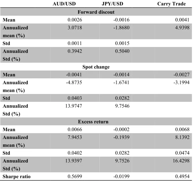
Table 1 shows the descriptive statistics of the AUD against USD, JPY against USD, and the carry trade strategy. From the table, we observe AUD/USD earn the higher excess return and higher volatility than JPY/USD, thus inducing positive carry trade excess return and high Sharpe ratio of 0.4954.[Table 1 about here] 2.2 Macroeconomic Variables
8
we select the following macro variables: (i) the growth rate of industrial production (ln IP
), (ii) inflation rate, (ii) real exchange rates, (iv) Taylor rule fundamentals. In the following, we provide some further motivation for these variables as predictors of carry trade returns. All data are obtained from Datastream.The growth rate of industrial production (ln IP
)This variable is based on industrial production growth differentials between Australia and Japan. More specifically, the growth differential is the IP growth rate of Australia minus the IP growth rate of Japan. The reasons why IP growth could matter can be summarized as below. First, IP growth has a natural interpretation in terms of business cycle risk and can serve as a proxy for risks from the real side of the macroeconomy. Second, from a risk-based asset pricing perspective, higher IP growth should be associated with lower marginal utility and causes a lower risk premium. Therefore, we expect to see low IP growth countries should have higher excess returns on average than high IP growth countries. Last reason is about that how IP growth might forecast currencies is analogous to growth stocks in equity markets. Past research shows that growth stocks underperform value stocks in international equity markets (Fama and French, 1998). While value and growth in equities are typically measured as the ratio of market to book value, there is no obvious counterpart to this in currency markets. However, the notion that the currencies of fast-growing countries are overvalued relative to currencies of slow-growing countries, just as growth stocks are overvalued relative to value stocks.
Inflation rate (ln CPI
)This variable is based on inflation differentials between Australia and Japan. More specifically, the inflation differential is the inflation rate of Australia minus the inflation rate of Japan. Guided by the connection between inflation and exchange
9
rates, we consider innovations in G7 inflation as explaining variable. Real exchange rates
One would expect that higher real exchange rates forecast higher excess returns in the future since higher real exchange rates indicate an undervaluation of a foreign currency relative to the USD. In this study, we use the real exchange rate of AUD against JPY as a predictable variable, which can be calculated as:
JPY
/ /
AUD
Real exchange rateAUD JPY Nominal exchange rateAUD JPY
CPI CPI
Taylor rule fundamentals
The use of Taylor rules to capture the set of fundamentals relevant for understanding exchange rate movements has been emphasized in recent literature (Engel and West, 2005, 2006; Molodtsova et.al., 2008). Drawing on this insight, we select Taylor rule fundamentals, TRF, and employ the following calibration:
ˆ 1.5 0.5
t t TRF y
for both home and foreign country where denotes the inflation rate and ˆy denotes the percent deviation of IP from a 5-period moving average. The calibrated parameters of 1.5 for inflation and 0.5 for the output gap are from what is often assumed in the Taylor rule literature. Taylor rule fundamentals basically serve to capture the determinants of policy rate controlled by monetary authority.
3. Methodology
In this section, we present the framework of regime switching model with time-varying transition probabilities.
3.1 Regime-switching model
Since 1989, Hamilton (1989) adopted the regime-switching model (RSM) to describe the business cycles in the U.S., there has been a surge of empirical research and
10
extension of the RSM. Due to the RSM can match the prosperity of financial markets to often change their behavior abruptly and the phenomenon that the new behavior of financial variables often persists for several periods after such a change, the RSMs are an important class of financial time series models. A key feature of the RSM is that model parameters are functions of a hidden Markov chain whose states represent hidden states of an economy, or different stages of business cycles. Engel and Hamilton (1990) and Engel (1994) have investigated quarterly changes in exchange rates and found the RSMs to be a good approximation to the underlying processes. Moreover, another studies that employed the RSM in exchange rates include Kirikos (2000), Caporale and Spagnolo (2004), Bergman and Hansson (2005), Ismail and Isa (2007) and Ichiue and Koyama (2011). For example, Bergman and Hansson (2005) suggest that the real exchange rate between the major currencies in the Post-Bretton Woods period can be described by a stationary, two state Markov switching AR(1) model. Ismail and Isa (2007) employ the RSM to capture regime shifts behavior in Malaysia ringgit exchange rates against four other currencies, namely the British pound sterling, the Australian dollar, the Singapore dollar and the Japanese yen, from 1990 to 2005. They conclude that the RSM is found to successfully capture the timing of regime shifts in the four series. Ichiue and Koyama (2011) confirm the RSM can also explain the most popular theme in the currency markets during the past decade, carry-trade. In the low exchange rate volatility regime, low-interest-rate currencies tend to depreciate and enable speculators to take more carry trade positions. While in the high exchange rate volatility regime consisting with the recent global financial meltdown, low-interest-rate currencies appreciate rapidly, causing investors liquidating their carry trade positions.
The basic idea of the RSM is that the model assigns probabilities to the occurrence of different regimes and the probabilities have to be inferred from the data. The
11
nonlinearity feature of the financial time series that can be in two or more regimes has motivated the used of RSMs. We model the joint distribution of a vector of n portfolio returns, rt
r r1t ...2t r nt
as a multivariate regime-switching process driven by a common discrete state variable s that takes integer values between 1 and k :t. t t s t r (1) Here 1 ... t t t s s ns
is a vector of mean returns in state s , and t
1...
0, t
t t nt N s
is the vector of return innovations that are assumed to be joint normally distributed with zero mean and state-specific covariance matrix
t
s
. Our assumption about the innovations to returns is thus capable to capturing time-varying volatilities and correlations in the joint distribution of asset returns (Timmermann, 2000; Manganelli, 2004; Patton, 2004). Each state is the realization of a first order Markov chain governed by the k k transition probability matrix
P with element pij defined as
1
Pr st i s| t j pij, ,i j1,..., .k (2)
The model (1)-(2) nests several popular models from the finance literature as special cases. In the case of single asset and two states, n1, k2, according to Engel and Hamilton (1990), the model could describe a variety of processes depending on the values taken by the six parameters
1,
2,
1,
2, p11 and p22. The state 1 andstate 2 represent currency depreciation and appreciation, respectively. When in the depreciation state, the mean value is 1, and the volatility is 1. On the other hand, in the state 2, the appreciation state, the mean value is 2, and the volatility is 2. The transition probability of appreciation-depreciation cycles can be defined by P.
12
Most importantly from their perspective is the ability of this model to capture so-called long swings in the exchange rate, which would be characterized by opposite signs on
1and
2 and large values of p11 and p22. Supposing that exchangerate is in the state 1 and that
1 is positive, under the long swings hypothesisexchange rate is expected to remain in the state 1 for 1/
1p11
periods and increase by
1 in each period. Once the state switches to the state 2, exchange rate isexpected to remain there for 1/
1p22
periods and to fall by
2 on average ineach period. Clearly this process has parallels with the desires of chartists to identify long-lived periods of currency appreciation or depreciation.
3.2 Time-varying transition probabilities
The unobserved state variable s is assumed to follow first-order Markov t
process with time-varying transition probabilities
| 1
1
ij t t t t
P s j s i p z (3) Where Ptij
is a function of a (k ) vector of observed exogenous or 1 predetermined variables zt1 , and
jPtij
1 i j,
1, 2 . In the present analysis, the observed information vector zt1 contains a constant and the macroeconomic variables described in the previous section.The transition probabilities are further assumed to be evolving as logistic function of
1
t
z . Specifically, the transition probability matrix is given as
13 with = exp ( ∙ ′ ) 1 + exp ( ∙ ), = 1 1 + exp ( ∙ ) = exp ( ∙ ′ ) 1 + exp ( ∙ ), = 1 1 + exp( ∙ )
Diebold, Lee, and Weinbach (1994) provide a tractable methodology to derive the maximum likelihood estimation based on an EM algorithm. They demonstrate that their extension to Hamilton’s Markov switching model by allowing for time-varying transition probabilities not only nests the framework with fixed transition probabilities but also better describes the true data generating process through simulation.
4. Empirical Results
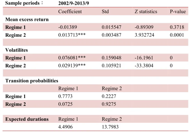
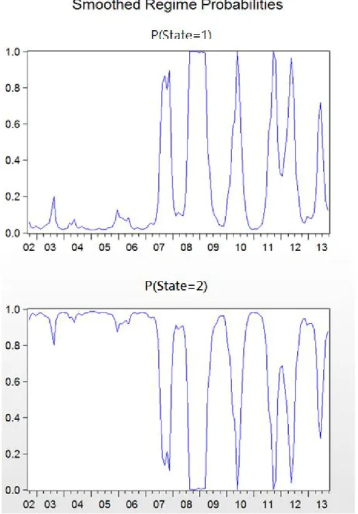
4.1 Evidence from regime switching model with constant transition probabilities Table 2 presents the parameter estimates of excess returns of carry trade strategy when using regime switching model with constant transition probabilities. Figure 1 plots the associated state probabilities. Regime 1 is a highly volatile bear state whose average duration is about 5 months and the mean returns on the carry trade strategy is non-significantly negative at -1.4% per month (-16.66% p.a.). Moreover, volatility is as high as 7.61% per month. During this regime, carry trade tend to be pulled back. Many investors turn away from commonly practiced carry-trade strategies and seek a “safe-haven” in these uncertain times, causing low-interest-rate currencies to appreciate rapidly, offsetting the profits gained from the differential in interest rates from the carry trade. Figure 1 shows that this regime captures major currency crashes and periods with sustained declined in currency values, such as the 2008 global financial crisis and the 2010 European sovereign debt crisis.
14
Regime 2 is a highly persistent low-volatility bull sate with an average duration of 14 months that captures long periods with relatively stable currency values during the late-2002 and the periods before the 2008 global financial crisis. Mean returns in this state are significantly positive at 1.4% (16.46% p.a.), hence the forward premium puzzle is strong and UIP is violated. Volatilities of returns at this regime is as low as 2.91% per month. Furthermore, the transition probabilities indicate that the market more easily exists to regime 2 from regime 1 (22.27%) than vice versa (7.25%).
[Table 2 about here] [Figure 1 about here]
4.2 Evidence from regime switching model with time-varying transition probabilities
In this section, we use the method of stepwise regression to select variables into the regime switching model with time-varying transition probabilities (TVTP). With univariate model, we find that only real exchange rate performs statistically significant. Next, we add the differentials of IP growth, the differentials of inflation rate, and the Taylor rule fundamentals with real exchange rate, respectively, to form three kinds of different models.
4.2.1 IP growth and real exchange rate
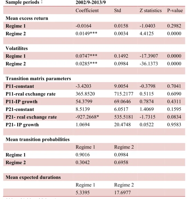
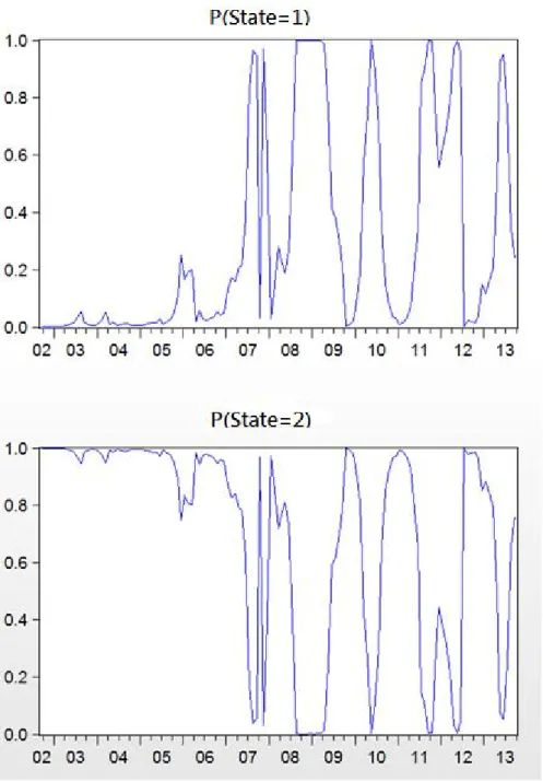
Table 3 presents the parameter estimates of excess returns of carry trade strategy with TVTP of IP growth and real exchange rate. Figure 2 plots the associated state probabilities. Similar with the results of constant transition probabilities, we still find two regimes. Regime 1 is a highly volatile bear state whose average duration is about 5 months and the mean returns on the carry trade strategy is non-significantly negative at -1.64% per month (-19.71% p.a.). Moreover, volatility is as high as 7.47% per month. Regime 2 is a highly persistent low-volatility bull sate with an average duration of 18 months and mean returns on the carry trade strategy is significantly
15
positive at 1.5% (17.83% p.a.). Volatilities of returns at this regime is as low as 2.85% per month. The time-varying transition probabilities results show that the coefficients of IP growth and real exchange rate on P are non-significantly positive at 54.3799 11
and 365.852, respectively. On the other hand, the coefficient of IP growth on P is 21
non-significantly positive at 1.0694. The only significant estimate is the coefficient of real exchange rate on P , which is negative at -927.2668. The results indicate the 21
real exchange rate can effectively predict the transition probabilities from bull state to bear state. The average P increases from 7.25% on table 2 to 30.42% on table 3. 21
Therefore, from figure 2, we can also observe more chances occurring from state 2 to state 1 compared with the results of figure 1.
[Table 3 about here] [Figure 2 about here] 4.2.2 Inflation rate and real exchange rate
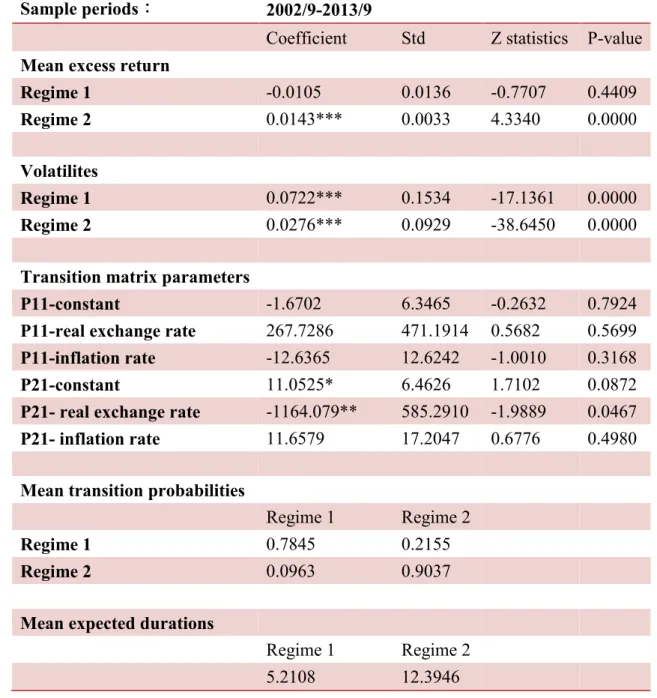
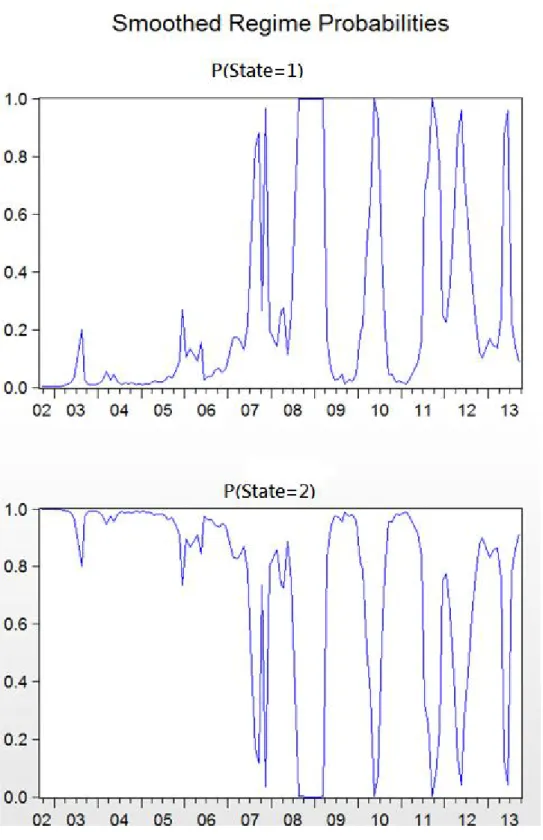
Table 4 presents the parameter estimates of excess returns of carry trade strategy with TVTP of inflation rate and real exchange rate. Figure 3 plots the associated state probabilities. Similar with the results of constant transition probabilities, we still find two regimes. Regime 1 is a highly volatile bear state whose average duration is about 5 months and the mean returns on the carry trade strategy is non-significantly negative at -1.05% per month (-12.6% p.a.). Moreover, volatility is as high as 7.22% per month. Regime 2 is a highly persistent low-volatility bull sate with an average duration of 12 months and mean returns on the carry trade strategy is significantly positive at 1.43% (17.16% p.a.). Volatilities of returns at this regime is as low as 2.76% per month. The time-varying transition probabilities results show that the coefficients of inflation rate and real exchange rate on P are non-significantly 11
16
coefficient of inflation rate on P is non-significantly positive at 11.6579. The only 21
significant estimate is the coefficient of real exchange rate on P , which is negative 21
at -1164.079. The results indicate the real exchange rate can effectively predict the transition probabilities from bull state to bear state. The average P increases from 21
7.25% on table 2 to 9.63% on table 4. Therefore, from figure 3, we can also observe more chances occurring from state 2 to state 1 compared with the results of figure 1.
[Table 4 about here] [Figure 3 about here] 4.2.3 Taylor rule fundamental and real exchange rate
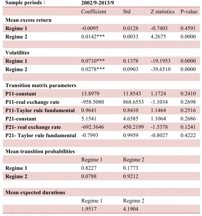
Table 5 presents the parameter estimates of excess returns of carry trade strategy with TVTP of Taylor rule fundamental and real exchange rate. Similar with the results of constant transition probabilities, we still find two regimes. Regime 1 is a highly volatile bear state whose average duration is about 2 months and the mean returns on the carry trade strategy is non-significantly negative at -0.95% per month (-11.4% p.a.). Moreover, volatility is as high as 7.1% per month. Regime 2 is a highly persistent low-volatility bull sate with an average duration of 4 months and mean returns on the carry trade strategy is significantly positive at 1.42% (17.04% p.a.). Volatilities of returns at this regime is as low as 2.78% per month. The time-varying transition probabilities results show that the coefficients of Taylor rule fundamental and real exchange rate on P are non-significantly positive at 0.9641 and negative at 11
-958.508, respectively. On the other hand, the coefficients of Taylor rule fundamental and real exchange rate on P are non-significantly negative at -0.7993 and -692.3646. 21
The results indicate that as Taylor rule fundamental combines information of both IP growth and inflation rate, its impact on transition probabilities might disappear through interaction between both variables, and might distort impact of real exchange rate on transition probabilities.
17
[Table 5 about here] 5. Conclusion
This paper examines the effects of the macroeconomic determinants on the returns of carry trade portfolio to be channeled through the transition probabilities in a Markovian process. From investing the carry trade returns by long Australian Dollar short Japanese Yen through the Markov regime switching model, we find two economic regimes can capture important time-variations in mean returns and volatilities of the excess returns of the above carry trade strategy. One state captures periods of low exchange rate volatility and high returns of the carry trade strategy, thus UIP is violated. The other regime captures the periods of high exchange rate volatility and non-significant negative return of the carry trade. Carry trade tend to be pulled back during liquidity shortages such as the recent global financial meltdown. Many investors turn away from commonly practiced carry-trade strategies and seek a “safe-haven” in these uncertain times, causing low-interest-rate currencies to appreciate rapidly, offsetting the profits gained from the differential in interest rates from the carry trade.
Next, we investigate the impacts of macroeconomic factors on carry trade performance through TVTP. We select several macroeconomic variables such as the growth rate of industrial production (ln IP
), inflation rate, real interest rate and Taylor rule fundamentals. Our results indicate the real exchange rate can effectively predict the transition probabilities from bull state to bear state. Through TVTP, we can also observe more chances occurring from bull state to bear state compared with the results with regime switching model with constant transition probabilities.18
References
Anzuini, A., Fornari, F., 2012. Macroeconomic Determinants of Carry Trade Activity, Review of International Economics 20, 468 – 488.
Backus, D.K., Foresi, S., Telmer, C., 2001. Affine term structure models and the forward premium anomaly. Journal of Finance 56 (1), 279–304.
Bakshi, G., Naka, A., 1997. On the unbiasedness of forward exchange rates. Financial Review 32, 145–162.
Bansal, R., 1997. An exploration of the forward premium puzzle in currency markets. Review of Financial Studies 10 (2), 369–403.
Bekaert, G., 1995. The time-variation of expected returns and volatility in foreign exchange markets. Journal of Business and Economic Statistics 13 (4), 397–408.
Bekaert, G., Hodrick, R.J., 1993. On biases in the measurement of foreign exchange risk premiums. Journal of International Money and Finance 12 (2), 115–138.
Bekaert, G., Wei, M., Xing, Y., 2007. Uncovered interest rate parity and the term structure. Journal of International Money and Finance 26 (6), 1038–1069.
Bergman, U.M., Hansson, J., 2005. Real exchange rates and switching regimes. Journal of International Money and Finance 24, 121-138.
Brennan, M.J., Xia, Y., 2006. International capital markets and foreign exchange risk. Review of Financial Studies 19 (3), 753–795.
Burnside, C., 2012. Carry trades and risk, in handbook of exchange rates (eds J. James, I. W. Marsh, L. Sarno), John Wiley & Sons, Inc., Hoboken, NJ, USA.
Caporale, G.M., Spagnolo, N., 2004. Modeling East Asian exchange rates: A Markov-switching approach. Applied Financial Economics 14, 233-242.
Chinn, M.D., Meredith, G., 2005. Testing uncovered interest parity at short and long horizons during the Post-Bretton Woods era. Manuscript. University of Wisconsin-Madison and International Monetary Fund.
19
Diebold, F. X., Lee, J. H., Weinbach, G., 1994. Regime-switching with time-varying transition probabilities. In C. Hargreves (Ed.), Nonstationary time series analysis and cointegration. Oxford: Oxford University Press.
Dumas, B., Solnik, B., 1995. The world price of foreign exchange risk. Journal of Finance 50 (2), 445–479.
Engel, C., 1994. Can the Markov switching model forecast exchange rates? Journal of International Economics 36, 151-165.
Engel, C., 1996. The forward discount anomaly and the risk premium: a survey of recent evidence. Journal of Empirical Finance 3 (2), 123–191.
Engel, C., Hamilton, J., 1990. Long swings in the dollar: are they in the data and do markets know it? The American Economic Review 80, 689-713.
Engel, C., West, K. D., 2005. Exchange Rates and Fundamentals, Journal of Political Economy 113, 485-517.
Engel, C., West, K. D., 2006. Taylor Rules and the Deutschmark-Dollar Real Exchange Rate, Journal of Money, Credit and Banking 38, 1175-1994.
Fama, E., 1984. Forward and spot exchange rates. Journal of Monetary Economics 14, 319–338.
Fama, E., French, K., 1998. Value versus Growth: The International Evidence, Journal of Finance 53, 1975-1999.
Flood, R., Rose, A., 1996. Fixes: of the forward discount puzzle. Review of Economics and Statistics 78 (4), 748–752.
Hamilton, J.D., 1989. A new approach to the economic analysis of nonstationary time series and the business cycle. Econometrica, 57, 357-384.
Hodrick, R., 1987. The empirical evidence on the efficiency of forward and futures foreign exchange markets. Harwood Academic Publishers, New York.
20
Trade Activity, Journal of Banking and Finance 37, 1133-1147.
Ichiue, H., Koyama, K., 2011. Regime switches in exchange rate volatility and uncovered interest rate parity. Journal of International Money and Finance 30, 1436-1450.
Ismail, M.T., Isa, Z., 2007. Detecting regime shifts in Malaysian exchange rates. Journal of Fundamental Science 3, 211-224.
Kirikos, D.G., 2000. Forecasting exchange rates out of sample: random walk v.s. Markov switching regimes. Applied Economics Letters 7, 133-136.
Lustig, H., Roussanov, N., Verdelhan, A., 2011. Common risk factors in currency markets. Review of Financial Studies 24, 3731-3777.
Menkhoff, L., Sarno, L., Schmeling, M., Schrimpf, A., 2012. Carry trades and global FX volatility. Journal of Finance 64, 681-718.
Molodtsova, T., Nikolsko-Rzhevskyy, A., Papell, D. H., 2008. Taylor Rules with Real-time Data: A Tale of Two Countries and One Exchange Rate, Journal of Monetary Economics 55, S63-S79.
Raffery, B., 2011. Currency returns, skewness and crash risk, manuscript. Duke University.
21
Table 1: Descriptive statistics
AUD/USD JPY/USD Carry Trade
Forward discout Mean 0.0026 -0.0016 0.0041 Annualized mean (%) 3.0718 -1.8680 4.9398 Std 0.0011 0.0015 Annualized Std (%) 0.3942 0.5040 Spot change Mean -0.0041 -0.0014 -0.0027 Annualized mean (%) -4.8735 -1.6741 -3.1994 Std 0.0403 0.0282 Annualized Std (%) 13.9747 9.7546 Excess return Mean 0.0066 -0.0002 0.0068 Annualized mean (%) 7.9453 -0.1939 8.1392 Std 0.0402 0.0282 0.0474 Annualized Std (%) 13.9397 9.7526 16.4298 Sharpe ratio 0.5699 -0.0199 0.4954
22
Table 2: Parameter estimates of the regime-switching model with constant transition probabilities for carry trade returns
Sample periods: 2002/9-2013/9
Coefficient Std Z statistics P-value Mean excess return
Regime 1 -0.01389 0.015547 -0.89309 0.3718 Regime 2 0.013713*** 0.003487 3.932724 0.0001 Volatilites Regime 1 0.076081*** 0.159048 -16.1961 0 Regime 2 0.029139*** 0.105921 -33.3804 0 Transition probabilities Regime 1 Regime 2 Regime 1 0.7773 0.2227 Regime 2 0.0725 0.9275
Expected durations Regime 1 Regime 2
4.4906 13.7983
23
Table 3: Parameter estimates of the regime-switching model with time-varying transition probabilities (TVTP) of IP growth and real exchange rate
Sample periods: 2002/9-2013/9
Coefficient Std Z statistics P-value Mean excess return
Regime 1 -0.0164 0.0158 -1.0403 0.2982
Regime 2 0.0149*** 0.0034 4.4125 0.0000
Volatilites
Regime 1 0.0747*** 0.1492 -17.3907 0.0000
Regime 2 0.0285*** 0.0984 -36.1373 0.0000
Transition matrix parameters
P11-constant -3.4203 9.0054 -0.3798 0.7041
P11-real exchange rate 365.8520 715.2177 0.5115 0.6090
P11-IP growth 54.3799 69.0646 0.7874 0.4311
P21-constant 8.5139 6.0517 1.4069 0.1595
P21- real exchange rate -927.2668* 535.5181 -1.7315 0.0834
P21- IP growth 1.0694 20.4748 0.0522 0.9583
Mean transition probabilities
Regime 1 Regime 2
Regime 1 0.9016 0.0984
Regime 2 0.3042 0.6958
Mean expected durations
Regime 1 Regime 2
5.3395 17.6977
24
Table 4: Parameter estimates of the regime-switching model with time-varying transition probabilities (TVTP) of inflation rate and real exchange rate
Sample periods: 2002/9-2013/9
Coefficient Std Z statistics P-value Mean excess return
Regime 1 -0.0105 0.0136 -0.7707 0.4409
Regime 2 0.0143*** 0.0033 4.3340 0.0000
Volatilites
Regime 1 0.0722*** 0.1534 -17.1361 0.0000
Regime 2 0.0276*** 0.0929 -38.6450 0.0000
Transition matrix parameters
P11-constant -1.6702 6.3465 -0.2632 0.7924
P11-real exchange rate 267.7286 471.1914 0.5682 0.5699
P11-inflation rate -12.6365 12.6242 -1.0010 0.3168
P21-constant 11.0525* 6.4626 1.7102 0.0872
P21- real exchange rate -1164.079** 585.2910 -1.9889 0.0467
P21- inflation rate 11.6579 17.2047 0.6776 0.4980
Mean transition probabilities
Regime 1 Regime 2
Regime 1 0.7845 0.2155
Regime 2 0.0963 0.9037
Mean expected durations
Regime 1 Regime 2
5.2108 12.3946
25
Table 5: Parameter estimates of the regime-switching model with time-varying transition probabilities (TVTP) of Taylor rule fundamental and real exchange rate
Sample periods: 2002/9-2013/9
Coefficient Std Z statistics P-value Mean excess return
Regime 1 -0.0095 0.0128 -0.7403 0.4591
Regime 2 0.0142*** 0.0033 4.2675 0.0000
Volatilites
Regime 1 0.0710*** 0.1378 -19.1953 0.0000
Regime 2 0.0278*** 0.0903 -39.6510 0.0000
Transition matrix parameters
P11-constant 13.8979 11.8543 1.1724 0.2410
P11-real exchange rate -958.5080 868.6553 -1.1034 0.2698 P11-Taylor rule fundamental 0.9641 0.8410 1.1464 0.2516
P21-constant 5.1541 4.6585 1.1064 0.2686
P21- real exchange rate -692.3646 450.2199 -1.5378 0.1241 P21- Taylor rule fundamental -0.7993 0.9959 -0.8027 0.4222 Mean transition probabilities
Regime 1 Regime 2
Regime 1 0.8227 0.1773
Regime 2 0.0788 0.9212
Mean expected durations
Regime 1 Regime 2
1.9517 4.1904
26
Figure 1: Smoothed regime probabilities with constant transition probabilities for carry trade returns
27
Figure 2: Smoothed regime probabilities with time-varying transition probabilities (TVTP) of IP growth and real exchange rate
28
Figure 3: Smoothed regime probabilities with time-varying transition probabilities (TVTP) of inflation rate and real exchange rate
科技部補助計畫衍生研發成果推廣資料表
日期:2016/03/24科技部補助計畫
計畫名稱: 利差交易報酬之總體經濟因素分析 計畫主持人: 林建秀 計畫編號: 103-2410-H-004-091- 學門領域: 財務無研發成果推廣資料
103年度專題研究計畫研究成果彙整表
計畫主持人:林建秀 計畫編號: 103-2410-H-004-091-計畫名稱:利差交易報酬之總體經濟因素分析 成果項目 量化 單位 備註(質化說明 :如數個計畫共 同成果、成果列 為該期刊之封面 故事...等) 實際已達成 數(被接受 或已發表) 預期總達成 數(含實際 已達成數) 本計畫實 際貢獻百 分比 國內 論文著作 期刊論文 0 0 100% 篇 研究報告/技術報告 1 1 100% 研討會論文 0 0 100% 專書 0 0 100% 章/本 專利 申請中件數 0 0 100% 件 已獲得件數 0 0 100% 技術移轉 件數 0 0 100% 件 權利金 0 0 100% 千元 參與計畫人力 (本國籍) 碩士生 4 4 100% 人次 博士生 0 0 100% 博士後研究員 0 0 100% 專任助理 0 0 100% 國外 論文著作 期刊論文 0 0 100% 篇 研究報告/技術報告 0 0 100% 研討會論文 0 0 100% 專書 0 0 100% 章/本 專利 申請中件數 0 0 100% 件 已獲得件數 0 0 100% 技術移轉 件數 0 0 100% 件 權利金 0 0 100% 千元 參與計畫人力 (外國籍) 碩士生 0 0 100% 人次 博士生 0 0 100% 博士後研究員 0 0 100% 專任助理 0 0 100% 其他成果 (無法以量化表達之 成果如辦理學術活動 、獲得獎項、重要國 際合作、研究成果國 際影響力及其他協助 產業技術發展之具體 效益事項等,請以文 字敘述填列。) 無成果項目 量化 名稱或內容性質簡述 科 教 處 計 畫 加 填 項 目 測驗工具(含質性與量性) 0 課程/模組 0 電腦及網路系統或工具 0 教材 0 舉辦之活動/競賽 0 研討會/工作坊 0 電子報、網站 0 計畫成果推廣之參與(閱聽)人數 0