2005 Deliverable Report:
Supply Chain Quadratic Goal Programming Models and Solutions
Task 1214.002: Robust Configuration and Monitoring of Semiconductor Supply Chains Contract 1214: Configuration, Monitoring and Control of Semiconductor Supply Chains
Task Leader: Argon Chen
Co-PI’s: David Chiang and Ruey-Shan Guo
Students: M.-C. Cheng, B.-C. Chang, C.-B. Chen, Jakey Lan, and Amos Hong 1. Abstract and Summary
This report presents a novel approach to formulating and optimizing the semiconductor supply chain performance. Unlike conventional modeling of supply chain operations, empirical quadratic models are established to describe the supply chain behavior. Quadratic goal programming model is then used to optimize the supply chain performance. In order to construct the quadratic response-surface models of supply chain performance, a supply chain simulation model is first set up. Simulation runs are then conducted based on a D-optimum experimental design. By the results of simulation experiments, quadratic models for different QoS priorities are built with stepwise regression. The quadratic response surfaces then serve as the objective functions of the goal programming model. Optimization is finally performed to obtain a robust supply chain configuration with its X-factors and cycle-time variability minimized.
2. Technical Results
2.1Semiconductor Supply Chain Simulation
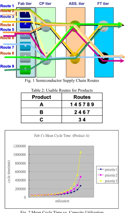
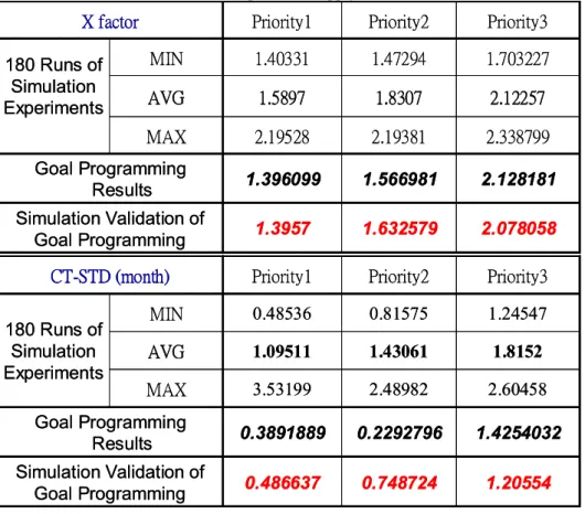
In this study, a four-tier semiconductor supply chain is simulated. The first tier is Fabrication (Fab); the second is Circuit Prob. (CP); the third is Assembly (Ass); and the fourth is Final Test (FT). There are six fabrication facilities and their corresponding capacities are designed to mimic 200mm foundry fabs of renowned companies, such as TSMC, and UMC (Table 1). Each of the CP, the ASS and the FT tier has two facilities available to the supply chain. There are nine available supply chain routes (Fig. 1) to serve three products, A, B and C. However, not all the available routes are usable to each type of the products (Table 2). Since the supply chain simulation model is an aggregated model, the most challenging task is to estimate the cycle time of a facility, especially of the fabrication facility, which usually consists of more than 300 processing steps. The cycle time can be divided into two portions: processing time and queue time. The processing times vary with the product type and the facility. The queue times are assumed to follow log-normal distributions with means varying with the capacity utilization and the QoS priority. Finally, the mean of the log-normal distribution is determined such that the mean cycle time appears to be an exponential function of the capacity utilization (Fig. 2). The simulation model is built using EM Plant . 2.2 Quadratic Response Surface Models
There are two types of input variables and two types of response variables for the supply chain response surface models. The input variables are also the decision variables for the goal programming. The first type of input variables is the route mix variable, ρkr. Route mix
ρkr represents the proportion of product k (k=1 for
Product A, 2 for Product B and 3 for Product C) demand to be allocated to supply chain route r. The second type of input variables is the priority mix variable, πkq.
Priority mix πkq denotes the proportion of product k
demand to be produced in QoS priority level q. In this study, there are three QoS priority levels: super hot lots (q=1), hot lots (q=2) and normal lots (q=3). The two types of response variables are to be used to evaluate the entire supply chain’s performance. The first type of variables is to measures the X-factor performance for each priority level. The second type of response variables is to measure the cycle time variability, i.e. cycle time standard deviation (CT-STD) in month. 180 runs of simulations chosen by D-optimum design are performed to obtain how the response variables are affected by the input variables. Stepwise regression is then used to select input variable terms, including linear, quadratic and interaction terms, into the response surface model. The resulting response surface models for QoS priority 1 are shown below. X-factor1= 3.04028 - 0.76932* ρ 18 - 5.32407* π 11* ρ 18 - 1.70306*ρ22 + 2.55627*π11*ρ22 - 3.21206*ρ24 + 2.0617*π11*ρ24 + 3.35593*ρ22* ρ24 + 6.45807*ρ24^2 - 6.01907*ρ26 + 2.64128*π11*ρ26 + 2.43013*ρ18* ρ26 + 3.95107*ρ22*ρ26 + 3.59718*ρ24*ρ26 + 6.27775*ρ26^2 - 2.08025*ρ 24*ρ33 + 0.95507*ρ33^2 - 0.89682*ρ22*π12 - 2.73278*ρ22*π21 - 2.94563* ρ24*π21 + 4.33951*π11*π31 +2.20954* ρ 22* π 31 + 2.26427* ρ 26* π 31 - 3.90953*ρ33*π31 +3.88601*π11*π32 – 0.69994*ρ33*π32 - 3.96577*π11*ρ11 – 1.57582* ρ22*ρ14 – 1.4345*ρ15 – 6.01892*π11*ρ15 + 4.19858*ρ26*ρ15 + 6.76398* π21*ρ15 CT-STD1= 10.76424 - 30.39664*ρ18 + 20.91593*ρ17*ρ18 + 44.38031*ρ18^2 - 7.04376*ρ22 +
3.75327* π 11* ρ 22 - 19.49143* ρ 17* ρ 22 - 14.41669*ρ24 - 19.90259*ρ17*ρ24 + 17.13541*ρ22*ρ24 + 19.52764*ρ24^2 - 16.44176* ρ26 - 20.93092*ρ17*ρ26 + 15.80926* ρ 22* ρ 26 + 16.97536* ρ 24* ρ 26 + 23.21307*ρ26^2 + 5.01638*ρ22*π22 - 6.09423*π31 + 9.03262*ρ22*π31 + 9.70458*ρ24* π31 + 7.29345*π12*π31 - 16.26179*ρ11 + 18.03107*ρ17*ρ11 + 27.58228*ρ 18*ρ11 - 5.73555*π12*ρ11 + 28.52365*ρ17*ρ14 + 29.47225* ρ 18* ρ 14 - 5.43344* ρ 22* ρ 14 + 23.20821*ρ11*ρ14 - 55.31215*ρ14^2 – 17.66627*ρ 15 + 17.71866*ρ17*ρ15 + 22.28432*ρ18*ρ15 + 11.24435* ρ 26* ρ 15 – 5.38951* π 22* ρ 15 + 32.58414*ρ11*ρ15 +25.65426*ρ14*ρ15
2.3 Quadratic Goal Programming Models
With the quadratic response surfaces to describe how the supply chain performance responds to changes of supply chain configurations, the response surfaces can be used as the goal functions in the goal programming. The goal objective function is then:
∑
= 3 1
i w (X-factori i + CT-STDi)
where wi is the weight for priority i products; X-factori is
the X-factor response surface for priority i and CT-STDi
is the CT-STD response surface for priority i. The constraints are listed below.
1. Product mix constraint:
∑ =
k k p 1
where pk is the proportion of product k demand in the
total demand and is given. 2. Priority mix constraints:
q p k k kq q ∀ ∑ ⋅π ≤φ k q kq ∀ ∑
π
= 1where φq is a preset upper limit for priority q proportion.
3. Route mix constraints: r pk rk r k ∀ ≤ ⋅ ∑ ρ α k r rk ∀ ∑ρ = 1
where αr is a preset upper limit for the proportion of total
demand to go through route r. 4. Capacity constraints:
(
ρ)
φ φ φ φ φ , : PT C t PT p E t t kt rk k r r k t⋅ ∑ ∑ ⋅ ⋅ ≤ ∀ ∈ whereEt is capacity utilization of supply chain tier t (an
economy factor);
Ctφ is proportion of facility f capacity in supply chain tier
t;
PTtφ is average bottleneck operation processing time by
facility f in supply chain tier t; and
PTktφ is average bottleneck operation processing time of
product k by facility f in supply chain tier t. 2.4 Supply Chain Optimization and Validation
With the quadratic goal programming model, optimization is performed using LINDO. Since the quadratic goal programming model has only linear constraints, the optimum solution found is ensured to be the global optimum. The results are shown in Table 3. The optimum supply chain route mix and priority mix settings are then validated through simulation and compared to the 180 simulation experiments in Table 4.
Table 1: Fab Capacity in Simulation Model
6465 k
Total689k
FAB61202k
FAB5z Capacity in 200mm wafers per year
z Fab1:TSMC 5, 6, or 8
z Fab2:UMC 8C, 8D, 8E, or 8F
z Fab3:TSMC 2
z Fab4:TSMC 3, 4, or 7
z Fab5:UMC 6A, or 8AB
z Fab6:WaferTech ,VIS , or SSMC
1133k
FAB4922k
FAB31376k
FAB21468k
FAB1 Capacity FAB6465 k
Total689k
FAB61202k
FAB5z Capacity in 200mm wafers per year
z Fab1:TSMC 5, 6, or 8
z Fab2:UMC 8C, 8D, 8E, or 8F
z Fab3:TSMC 2
z Fab4:TSMC 3, 4, or 7
z Fab5:UMC 6A, or 8AB
z Fab6:WaferTech ,VIS , or SSMC
1133k
FAB4922k
FAB31376k
FAB21468k
FAB1 Capacity FAB1 2 3 4 5 6 1 2 1 2 1 2
Fab tier CP tier ASS. tier FT tier
Route 4 Route 3 Route 1 Route 5 Route 6 Route 7 Route 9 Route 8 Route 2 1 2 3 4 5 6 1 2 1 2 1 2
Fab tier CP tier ASS. tier FT tier
Route 4 Route 4 Route 3 Route 3 Route 1 Route 1 Route 5 Route 5 Route 6 Route 6 Route 7 Route 7 Route 9 Route 9 Route 8 Route 8 Route 2 Route 2
Fig. 1 Semiconductor Supply Chain Routes Table 2: Usable Routes for Products
3 4
C
2 4 6 7
B
1 4 5 7 8 9
A
Routes
Product
3 4
C
2 4 6 7
B
1 4 5 7 8 9
A
Routes
Product
Fab-1's Mean Cycle Time (Product A)
0 200000 400000 600000 800000 1000000 1200000 utilization cy cl e tim e( m in ) priority1 priority2 priority3
Fig. 2 Mean Cycle Time vs. Capacity Utilization Table 3 Optimum Supply Chain Configuration
0.15 0.25 0.6 0.05 0.25 0.7 0.05 0.1 0.85 Priority 1 Priority 2 Priority 3 Product 3 Product 2 Product 1 Priority Mix 0.15 0.25 0.6 0.05 0.25 0.7 0.05 0.1 0.85 Priority 1 Priority 2 Priority 3 Product 3 Product 2 Product 1 Priority Mix Product 1 Route Mix 0.254671 0.183181 0.147153 0.114994 0.1 0.2 Route 9 Route 8 Route 7 Route 5 Route 4 Route 1 Product 1 Route Mix 0.254671 0.183181 0.147153 0.114994 0.1 0.2 Route 9 Route 8 Route 7 Route 5 Route 4 Route 1 Product 2 Route Mix 0.364144 0.3 0.235856 0.1 Route 7 Route 6 Route 4 Route 2 Product 2 Route Mix 0.364144 0.3 0.235856 0.1 Route 7 Route 6 Route 4 Route 2 Product 3 Route Mix 0.470714 0.529286 Route 4 Route 3 Product 3 Route Mix 0.470714 0.529286 Route 4 Route 3
Table 4: Validation of Optimized Supply Chain Performance