可調視訊編碼位元流擷取之最佳化

國 立 交 通 大 學

資訊科學與工程研究所

碩 士 論 文

可調視訊編碼位元流擷取之最佳化

Optimized Extraction for SVC Bit-streams

研 究 生：黃淩軒

指導教授：邵家健 副教授

彭文孝 助理教授

可調視訊編碼位元流擷取之最佳化

Optimized Extraction for SVC Bit-streams

研 究 生：黃淩軒

Student：Lin-Shung Huang

指導教授：邵家健

Advisors：John Kar-Kin Zao

彭文孝 Wen-Hsiao

Peng

國 立 交 通 大 學

資 訊 科 學 與 工 程 研 究 所

碩 士 論 文

A Thesis

Submitted to Institute of Computer Science and Engineering College of Computer Science

National Chiao Tung University in partial Fulfillment of the Requirements

for the Degree of Master

In

Computer Science

August 2007

Hsinchu, Taiwan, Republic of China

可調視訊編碼位元流擷取之最佳化

學生：黃淩軒

指導教授：邵家健

彭文孝

國立交通大學資訊科學與工程研究所 碩士班

摘 要

我們的研究目的是提出一個最佳化的可調視訊編碼的位元流擷取方法，主 要是能夠針對不同的播放設備以及網路頻寬調整擷取的位元流內容，使不同頻 寬之下仍能提供最理想的播放畫質。 我們分析可調視訊編碼的位元流之編碼相依性限制，進而提出兩種方法來 產生的擷取路徑：一、Convex Sets 限制每一步擷取必須包含所有編碼相依的資 料，使位元流可以完整的解碼；二、Wavefront Sets 容許每一步擷取可以包含仍 無法解碼的資料，但擷取路徑仍不違反編碼相依性。另外，針對異質接收端的 各種播放設備的畫面大小與畫率可能不盡相同，我們提出一個模擬不同播放設 備的方法，使量測到的失真值能夠較接近真實播放畫面的失真。 為了得到最佳化的播放畫質，我們提出兩種方法來選擇最佳擷取路徑：一、 Global Optimal；二、Local Optimal。我們實作出一個位元流擷取路徑的測試平 台，並針對不同的視訊內容、不同的播放設備、和不同的擷取路徑進行測試與 分析。我們從實驗結果得到幾項結論：一、不同的擷取路徑確實會造成不同的 播放品質；二、最佳化的擷取路徑因視訊內容與播放設備而異；三、利用 Convex Set 測試時，Local Optimal 與 Global Optimal 可得到相同結果；四、利用 Wavefront Sets 與 Convex Sets 所選擇的 Global Optimal 結果是吻合的。

最後，我們將最佳化之位元流擷取方法運用於異質網路中的視訊傳輸。我 們提出一個分散式視訊群播的系統架構，並探討如何在伺服端以及接收端進行 資源分配。

Optimized Extraction for SVC Bit-streams

Student：Lin-Shung

Huang

Advisors：John Kar-Kin Zao

Wen-Hsiao Peng

Institute of Computer Science and Engineering

National Chiao Tung University

ABSTRACT

Our research goal is to propose an optimized extraction scheme for SVC bit-streams for different device types. The basic principle of extraction path optimization is to minimize the distortion of the reconstructed frames while the rate increases.

We presented two methods for extracting path permutations: (1) through the use of Wavefront Sets that allow incomplete bit-streams, as long as not violating the coding dependencies; and (2) through the use of Convex Sets that extract completely decodable bit-streams. We also introduced two path optimization methods: (1) via global optimization and (2) local optimization. We evaluate the possible extraction paths and choose the optimal according to their device-specific rate-distortion performances.

From experimental results, we conclude that: (1) Different device types result in different optimal extraction paths; (2) Different content types result in different optimal extraction paths; (3) Global optimal provides the same results as local method when using the convex method. (4) Convex sets provides the same results as wavefront sets when finding the global optimal.

We propose a SVC-based multisource streaming scheme, applying optimized extraction. We present bandwidth request/allocation algorithms for servers and clients using heuristic solutions.

誌 謝

首先我要感謝邵老師與彭老師一直以來給予我研究上的指導，若不是經由 不斷地與老師的討論，以及兩位老師給予指引與協助，我將無法順利完成這些 工作。這兩年來，老師的教導，無論是研究方法或是待人處事，都令我獲益良 多。對於老師平時給我的鼓勵與支持，我真的感激不盡。另外，我要感謝呂俊 賢學弟協助重畫了論文中的一些數據圖；感謝林鴻志學長解答了我對 JSVM 軟 體的一些疑問；感謝黃國晉學長、李明龍同學、黃雪婷學妹參與每次的討論； 還要感謝彭老師實驗室的同學給予我口試上的寶貴意見。感謝所有 PES 實驗室 的成員與學長們，包含黃國晉、朱書玄、張哲維、劉育志、李明龍、郭芳伯、 曾輔國、林哲民、郭宇軒、龔哲正、吳事修、陳亦興以及 Lily，能夠在認真研 究之餘也帶來歡笑，你們是我最好的伙伴。最後我要感謝一直默默支持著我的 家人，謝謝你們！

C

ONTENTS

摘要 ... I ABSTRACT...II 誌謝 ... III CONTENTS... IV

Chapter 1 Research Overview ... 1

1.1 Introduction...1

1.2 Problem Statement ...1

1.3 Research Approach ...2

1.4 Thesis Outline ...3

Chapter 2 Background ... 4

2.1 Scalable Video Coding...4

2.1.1 Encoder Overview ...4

2.1.2 Hierarchical-B Prediction Structure...6

2.1.3 Inter-layer Prediction Structure...6

2.1.4 Network Abstraction Layer...7

2.2 Related Work...9

2.2.1 Quality Index Optimized Extraction...9

2.2.2 Perceptual Quality Optimized Extraction ...10

2.2.3 Quality Layers Optimized Extraction ...12

Chapter 3 Optimized Extraction ... 15

3.1 Bit-stream Extraction ...15

3.1.1 Extraction Path...15

3.1.2 Basic Unit for Extraction ...17

3.2 Path Permutation...22 3.2.1 Wavefront Sets ...23 3.2.2 Convex Sets ...24 3.3 Path Optimization ...26 3.3.1 Global Optimal...27 3.3.2 Local Optimal ...28 3.4 Distortion Measurement...28 3.4.1 Device Simulation...28 3.5 Program Architecture ...29 3.6 Extraction Framework ...31 Chapter 4 Experiments... 32 4.1 System Configuration ...32 4.2 Experimental Method...32

4.3 Results and Analysis ...33

4.3.1 Comparison of Extraction Paths ...33

4.3.2 Comparison of Device Types ...34

4.3.3 Comparison of Test Sequences ...36

4.3.4 Comparison of Wavefront and Convex Sets ...37

4.3.5 Comparison of Global and Local Optimal...38

4.3.6 Deduction of Optimal Paths for Different Devices...39

4.3.7 R-D Performance of Sub-layers...40

Chapter 5 Multisource Streaming ... 43

5.1 Introduction...43

5.2 Coding Scheme ...45

5.3 Negotiation Protocol ...47

5.5 Client Scheme ...49 5.5.1 Rate Allocation...50 5.5.2 Server Selection ...52 Chapter 6 Conclusion... 54 6.1 Accomplishment ...54 6.2 Future Work ...55 REFERENCE... 56

Chapter 1 Research Overview

1.1 Introduction

Nowadays, heterogeneous networks are becoming more popular and multimedia streaming services has emerged as one of the most desired applications. In such environments, the users are connected to the Internet through a wide range of network links, such as 3G, WiMax and WLan. The network condition of each user may vary greatly in the bandwidth and reliability. Furthermore, the characteristics of pervasive user devices are very diverse, such as cell phones, PDA, PC and HDTV. Each device type supports different features in display capabilities, processing power, power supplies and storage. Considering such heterogeneous environments, how to efficiently provide multimedia services is an interesting research area.

1.2 Problem Statement

From source coding perspective, the variation of network bandwidth and the population of user devices are unpredictable at the encoding stage. To serve diversified clients with traditional video coding techniques, the same video content would have to be encoded several times, targeting different bit-rates and resolutions. However, distributing multiple bit-streams of the same video content is wasteful, because there is a lot of redundancy between the different versions.

To provide effective video streaming service over heterogeneous networks, scalable video coding has become an essential technology in video coding for serving the same video content to multiple target user devices using a single bit-stream. The goal of scalable video coding is to allow flexible bit-stream adaptation and provide decodable bit-streams at different bit-rates and to different

target user devices while matching the user preferences. In our research, we will focus on how to make the appropriate adaptation decisions to achieve the best possible video quality for multiple user devices.

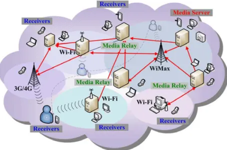
Next, we consider applying optimized extraction to the video transmission scenario depicted in Figure 1. In this scenario, the media server is the source of the media stream. Multiple media relays across the network are organized to help achieve a higher overall throughput to the clients. Varying numbers of receivers are connected to the media streaming service through different network links. Given the heterogeneity of the network, how to achieve effective bandwidth usage for video transmission is an important issue.

Figure 1: Transmission scenario

1.3 Research Approach

Scalable video coding (SVC) has been proposed to serve diversified clients with a single bit-stream. SVC allows partial bit-streams to be extracted from a scalable bit-stream while achieving reduced temporal, spatial or SNR resolutions.

minimum distortion for different bit-rates and devices. Our approach is to use optimal extraction paths to indicate the optimized order of enhancing the spatial, temporal or SNR resolution while the bit-rate increases. The optimal extraction paths can be pre-processed and later be used to perform on-the-fly adaptation decisions.

The basic principle of extraction path optimization is to minimize the distortion of the reconstructed frames while the rate increases. We present two concepts for possible path permutation: (1) wavefront sets and (2) convex sets. Then we introduce two methods for path optimization: (1) global optimal and (2) local optimal. We evaluate all possible extraction paths and choose the optimal according to their rate-distortion performances.

We will apply our results of optimized extraction to propose a flexible multisource streaming scheme. We will focus on discussing the bandwidth request/allocation algorithms of the media gateways and clients using heuristic solutions.

1.4 Thesis Outline

In Chapter 2, we will briefly introduce the basics of scalable video coding (SVC). In Chapter 3, we will discuss the details of bit-stream extraction optimization. In Chapter 4, we will present the experimental results and our analysis. In Chapter 5, we will propose a heuristic bandwidth allocation algorithm for SVC multisource streaming. In Chapter 6, we will present our conclusion and future work.

Chapter 2 Background

2.1 Scalable Video Coding

The scalable video coding (SVC) standard [1] is an extension of the H.264/AVC standard [2] developed by the Joint Video Team (JVT) that uses a single bit-stream to provide multiple frame rates, frame sizes and quality levels while achieving a reasonable coding efficiency.

SVC provides three types of scalabilities: (1) Spatial scalability allows multiple frame sizes. (2) Temporal scalability allows multiple frame rates. (3) SNR scalability allows multiple quality levels. SNR scalability consists of coarse grain scalability (CGS) and fine grain scalability (FGS), which allows flexible truncation of the coded data. SVC supports combined scalability, such that all three types of scalability can be easily combined to support a wide range of spatial, temporal and SNR scalabilities.

The coded data of SVC bit-streams are organized as multiple layers. The base layer provides the basic video quality at the minimum supported bit rate. The enhancement layers successively refine the video quality. SVC provides flexible bit-stream extraction to obtain the desired resolutions or bit-rates on-the-fly.

2.1.1 Encoder Overview

This section presents an overview of the SVC encoder. The encoding is based on a layered approach that uses separate encoder loops for each layer and uses adaptive inter-layer prediction techniques to exploit correlations among the layers. Spatial scalability and CGS are achieved by multiple layers with a pyramid structure. Temporal scalability is achieved by a temporal decomposition using hierarchical B

pictures. FGS is achieved by encoding successive refinements of the transform coefficients.

Figure 2 [3] depicts an example of an SVC encoder with three spatial layers. Each layer is encoded with separate encoder loops, as shown in the dotted boxes.

Prediction Picture Buffer Deblocking Filter IQIDCT Entropy Coding DCTQ Pred. error Motion information Pred. image texture residue Inter-layer scale Inter-layer scale

texture/motion/residue _{(AVC compatible)}Base layer Prediction Picture Buffer Deblocking Filter IQIDCT Entropy Coding DCTQ Pred. error Motion information Pred. image texture residue Inter-layer scale Inter-layer scale

texture/motion/residue First Enh-layer

Prediction Picture Buffer Deblocking Filter IQIDCT Entropy Coding DCTQ Pred. error Motion information Pred. image texture residue Inter-layer scale Inter-layer scale texture/motion/residue M U X SVC bitstream Input Video Second Enh-layer Prediction Picture Buffer Deblocking Filter IQIDCT Entropy Coding DCTQ Pred. error Motion information Pred. image texture residue Inter-layer scale Inter-layer scale

texture/motion/residue _{(AVC compatible)}Base layer

Prediction Picture Buffer Deblocking Filter IQIDCT Entropy Coding DCTQ Pred. error Motion information Pred. image texture residue Inter-layer scale Inter-layer scale

texture/motion/residue _{(AVC compatible)}Base layer Prediction Picture Buffer Deblocking Filter IQIDCT Entropy Coding DCTQ Pred. error Motion information Pred. image texture residue Inter-layer scale Inter-layer scale

texture/motion/residue First Enh-layer

Prediction Picture Buffer Deblocking Filter IQIDCT Entropy Coding DCTQ Pred. error Motion information Pred. image texture residue Inter-layer scale Inter-layer scale

texture/motion/residue First Enh-layer

Prediction Picture Buffer Deblocking Filter IQIDCT Entropy Coding DCTQ Pred. error Motion information Pred. image texture residue Inter-layer scale Inter-layer scale texture/motion/residue Prediction Picture Buffer Deblocking Filter IQIDCT Entropy Coding DCTQ Pred. error Motion information Pred. image texture residue Inter-layer scale Inter-layer scale texture/motion/residue M U X SVC bitstream Input Video Second Enh-layer

Figure 2: SVC encoder structure with three spatial layers [3]

The input video is spatially scaled to support multiple spatial resolutions. For each spatial layer, the prediction comes from either temporally neighbored pictures at the same layer or spatially up-sampled pictures from lower layers. The inter-layer prediction scheme can reuse the texture, motion and residue information of the lower layers to improve the coding efficiency. After the prediction scheme, the transform coefficients at each spatial layer are encoded with either a scalable entropy coder for FGS or a non-scalable entropy coder for CGS.

2.1.2 Hierarchical-B Prediction Structure

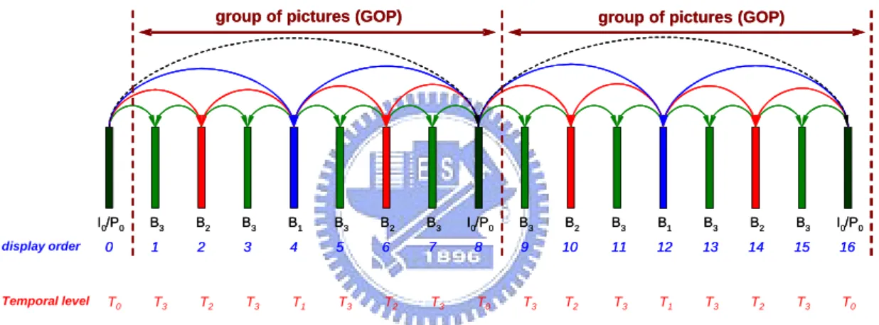
SVC uses hierarchical-B prediction structure to support multilevel temporal scalability. Figure 3 depicts a hierarchical-B prediction structure with 4 temporal levels and a GOP size of 8. Each key picture (black) is either an intra-coded I-frame or a P-frame that uses the previous key picture as the reference picture. Each B-frame is bi-directionally predicted using both previously and future displayed reference pictures from the lower temporal level. The pictures are hierarchically predicted as illustrated.

I₀/P₀ B₃ B₂ B₃ B₁ B₃ B₂ B₃ I₀/P₀ B₃ B₂ B₃ B₁ B₃ B₂ B₃ I₀/P₀

0 1 2 3 4 5 6 7 8 9 10 11 12 13 14 15 16

group of pictures (GOP) group of pictures (GOP)

I₀/P₀ B₃ B₂ B₃ B₁ B₃ B₂ B₃ I₀/P₀ B₃ B₂ B₃ B₁ B₃ B₂ B₃ I₀/P₀

0 1 2 3 4 5 6 7 8 9 10 11 12 13 14 15 16

display order

group of pictures (GOP) group of pictures (GOP)

T0 T3 T2 T3 T1 T3 T2 T3 T0 T3 T2 T3 T1 T3 T2 T3 T0

Temporal level

Figure 3: Hierarchical-B prediction structure with a GOP size of 8

The pictures of lower temporal levels are encoded first such that the pictures of higher temporal levels can refer to the reconstructed pictures at lower layers. The higher temporal levels are not required for the decoding of the lower temporal levels. Each GOP can be independently decoded if the preceding key picture is available.

2.1.3 Inter-layer Prediction Structure

The inter-layer prediction structure is be configured according to the types of layers used. The spatial and CGS layers can flexibly select the reference layer from any lower layers while the FGS layers must be predicted from the previous SNR

layer at the same resolution.

Figure 4 [3] depicts an example of inter-layer prediction with three spatial layers. Each spatial resolution contains several SNR layers. In the first column, BASE_0_0 is the base layer of spatial layer 0. On top, CGS_1_0 and CGS_2_0 are encoded as CGS layers, which are predicted from BASE_0_0 and CGS_1_0, respectively. BASE_0_0 CGS_1_0 CGS_2_0 BASE_3_0 CGS_4_0 FGS_4_1 BASE_5_0 FGS_5_1 FGS_4_2

Spatial layer 0 Spatial layer 1 Spatial layer 2 FGS_5_2 BASE_0_0 CGS_1_0 CGS_2_0 BASE_3_0 CGS_4_0 FGS_4_1 BASE_5_0 FGS_5_1 FGS_4_2

Spatial layer 0 Spatial layer 1 Spatial layer 2 FGS_5_2

Figure 4: Inter-layer prediction structure with three spatial layers [3]

Note that SVC allows flexible selection of reference layers, such that decoding a certain layer may not need all of its lower layers. As shown, CGS_4_0 refers to CGS_2_0 instead of BASE_3_0, while BASE_3_0 refers to CGS_1_0 instead of CGS_2_0. Therefore, CGS_2_0 is not necessary for decoding BASE_3_0, while BASE_3_0 is not necessary for decoding CGS_4_0. Such flexibility leaves room for further optimizations on performance or error resilience.

2.1.4 Network Abstraction Layer

The elementary unit for the output of an SVC encoder and the input of an SVC decoder is a network abstraction layer (NAL) unit. The NAL unit structure is designed to provide convenient packetization of coded video data for different

transport layers or storage media. NAL units can be categorized into two types: „ Video coding layer (VCL) NAL

VCL NAL units contain the coded data of video pictures, such as coded slice, coded slice data partition and suffix NAL units. A coded slice NAL unit contains data of one or more coded macroblocks. A coded slice data partition NAL unit contains partitioned data of a coded slice. A suffix NAL unit contains descriptive information of the preceding NAL unit.

„ Non-VCL NAL

Non-VCL NAL units contain associated information such as parameter sets and supplemental enhancement information (SEI). Parameter sets contain infrequently changing information that is essential for decoding sequences of video pictures. SEI messages contain additional information that are not required for decoding but assist in related process such as frame output timing, error concealment, and resource reservation. Non-VCL NAL units can be sent out-of-band using a more reliable transport mechanism.

The NAL unit consists of a header followed by a byte string of payload data. Figure 5 [4] depicts the SVC NAL header, which consists of the one-byte H.264/AVC header and the three-byte SVC extension header.

Each NAL unit belongs to certain scalability levels and is tagged with the syntax elements dependency_id, temporal_level and quality_level. In SVC, a layer is defined as a set of NAL units with the same value of dependency_id.

„ The syntax element dependency_id indicates the layer identifier of spatial and CGS layers.

„ The syntax element temporal_level indicates the hierarchical level of temporal prediction, which relates to the frame rate.

„ The syntax element quality_level indicates the quality level of FGS layers.

2.2 Related Work

2.2.1 Quality Index Optimized Extraction

The quality index optimized extraction [5] is proposed in a sense that the quality index (QI) of an extracted bit-stream is maximized for the given network bandwidth constraint. The quality index is an optimality index in terms of PSNR-based objective visual quality and MOS-based subjective perceptual quality.

The total QI is defined as a weighted measure of spatial, temporal and SNR scalability QI’s as follows:

(

si fj qk

)

ws QISR

( )

si wf QIFR

( )

fj wq QIPSNR

(

si fj qk

)

QI , , = ⋅ + ⋅ + ⋅ , ,

The parameters , and indicate the weighting factors of the three

quality indexes QI , s w

(

i SR s f w

)

q w

( )

fj FR

QI and QI_PSNR

(

s_i, f_j,q_k

)

, respectively. The parameters , and indicate that the SVC bistream is extracted at the

spatial scalability level, the temporal scalability level and the SNR scalability level. The optimization-theoretic approach extracts a bit-stream in the

i

s f _j q_k

th

sense that the total QI is maximized without exceeding the maximum bit-rate B_max. The QI for SNR scalability is measured in terms of PSNR values. The QI for spatial scalability is considered as the perceptual quality of different resolutions. To simplify the problem, the video pictures with lower spatial resolutions are interpolated into the highest spatial resolution and then measured in terms of the PSNR values. The QI for temporal scalability is defined as the perceptual quality of different frame rates and is measured with a five grade scale. The expo-logarithm function shown in Figure 6 [5] is utilized to model the QI for temporal scalability.

Figure 6: Temporal QI modeling with expo-logarithm functions [5]

The quality index optimized extraction shows better performance than extracting the closest bit-rate at different bit-rates. However, the quality index is not capable of modeling playback quality on different target device types. The layer switching problem is also an issue, however not mentioned in this paper.

2.2.2 Perceptual Quality Optimized Extraction

The perceptual quality optimized extraction [6] performs extraction using perceptual quality preference path depending on video class. This work analyzes that video segments belonging to the same video class have consistent characteristic of

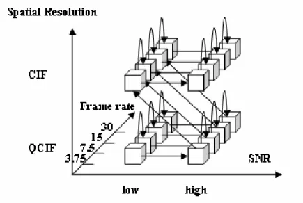
quality preference. The video segments are classified into different classes, namely action, crowd, dialog, scenery, and text & graphic. Based on subjective tests on the quality preference in these five video classes, quality information tables (QIT) were determined. The QITs are applied to bit-stream extraction to maximize the perceptual quality according to video class. In Figure 7 [6], the preference paths for each video class as bit-rate decreases are shown in three-dimensional scalability.

Figure 7: Preference path: (a) scenery, (b) action, (c) crowd, (d) text & graphic [6]

From the results of this paper, we consider the video class as an important factor for determining the perceptual quality preference paths. We extend this idea

by testing different video classes on different device types for optimizing the preference paths.

2.2.3 Quality Layers Optimized Extraction

Quality Layers optimized extraction [7] is proposed such that the impact on rate and distortion of each coded picture is evaluated to help perform optimized extraction for SNR enhancement layers. Figure 8 [7] depicts the rate-distortion curve with the coordinates representing the rate and distortion values calculated for each picture. The points lying on the convex hull of the curve are sorted according to their rate-distortion slope. The NAL units are prioritized according to this curve, such that the pictures with lower rate-distortion performances are truncated first

Figure 8: Rate-distortion curve [7]

The distortion of each SNR enhancement picture is computed by two methods: „ Independent Distortion

For open-loop coding, it is assumed that the impact of different pictures on the distortion of the reconstructed sequence is uncorrelated. The distortion for each SNR enhancement picture is calculated by decoding at the selected quality_level without the lower temporal layers. The impact on the

distortion is measured as the difference of the reconstructed sequence with and without a particular SNR layer.

„ Dependent Distortion

For closed-loop coding, the distortion of each reconstructed picture depends on the distortion of its reference pictures. The distortion for each picture is calculated by decoding at the selected quality_level with the required lower temporal layers. The impact on the distortion is measured as the difference of the reconstructed sequence with and without a particular temporal layer.

Figure 9 [7] depicts the truncation orders of NAL units using Quality Layers optimized extraction. Each of the big blocks represents a set of NAL units with dependency_id i, temporal_level j and quality_level k, labeled as (Ri,Tj,Qk). Each of the small blocks represents an NAL unit belonging to an SNR enhancement layer. As shown, the NAL units of the base layers (quality_level = 0) are always prioritized first. The NAL units of the SNR enhancement layers are ordered according to the rate-distortion performance of each picture. Note that the priorities of NAL units are not strictly assigned at layer boundaries. Note that pictures of a higher quality_level (R0, T2, Q2) may be truncated before pictures of a lower quality_level (R1, T2, Q1).

Figure 9: Quality Layers truncation order [7]

The Quality Layers extraction shows improvement over the simple truncation method in JSVM [8]. However, the distortion is measured in an approximated way, not considering the fact that the truncation order will also affect the actual distortion of the reconstructed sequence. We suspect that truncating according to the rate-distortion performances measured this way may not ensure the optimal distortion of the reconstructed sequence. We propose an extension to the idea of rate-distortion optimization specifically for non-FGS layers and for different device types, while considering the truncation order when evaluating rate-distortion performance.

Chapter 3 Optimized Extraction

3.1 Bit-stream Extraction

A scalable SVC bit-stream can be organized to support multiple spatial, temporal and SNR resolutions. Starting from the global bit-stream with maximum spatial, temporal, and SNR resolutions, partial bit-streams can be extracted and decoded at reduced resolutions. This section discusses the details of SVC bit-stream extraction.

3.1.1 Extraction Path

In this article, we use the term extraction path as a sequence of incrementing extraction steps. Extraction paths indicate the order of enhancing the spatial, temporal or SNR resolution while the bit-rate increases. For a scalable bit-stream with combined scalability, there are normally more than one possible extraction paths.

Figure 10 depicts several possible extraction paths for an example bit-stream. Each spatio-temporal-quality cube represents a supported spatial, temporal and SNR resolution. All extraction paths start from the minimum spatio-temporal resolution at the minimum bit-rate. All extraction paths end with the maximum spatio-temporal resolution at the maximum bit-rate. Moving through the spatial-temporal-quality cubes represents increasing the spatial, temporal or SNR resolution.

Generally, when the target bit-rate increases, the decoded video quality improves. When the target bit-rate decreases, the decoded video quality decreases. The decoded video quality should never decrease when the bit-rate increases.

Figure 10: Spatio-temporal-quality cube with possible extraction paths

Layer Switching Problem

Layer switching occurs when the spatial or CGS scalability level of the extracted bit-stream either increases or decreases as the bit-rate changes. For switching from layer k to layer k-1, the decoder has no problem decoding layer k-1, since the lower layers 0 ~ k-1 were already decodable when it was decoding layer k. However, for switching from layer k to layer k+1, the decoder may not be able to decode the layer k+1. This is because the key pictures of the layer k+1 may refer to previous pictures of the layer k+1, which were not provided to the decoder before layer switching.

To solve this problem, SVC allows encoding IDR pictures independently for each layer. However, frequent coding of IDR pictures causes reduced coding efficiency. We assume that the key pictures of higher layers are coded with IDR pictures for every constant number of GOPs, such that layer switching is allowed at GOP boundaries.

3.1.2 Basic Unit for Extraction

In SVC, bit-streams are consisted of NAL units. Each NAL unit belongs to certain scalability levels and is tagged with the syntax elements dependency_id, temporal_level and quality_level. Bit-stream extraction is to extract NAL units for the required scalability levels or bit-rate.

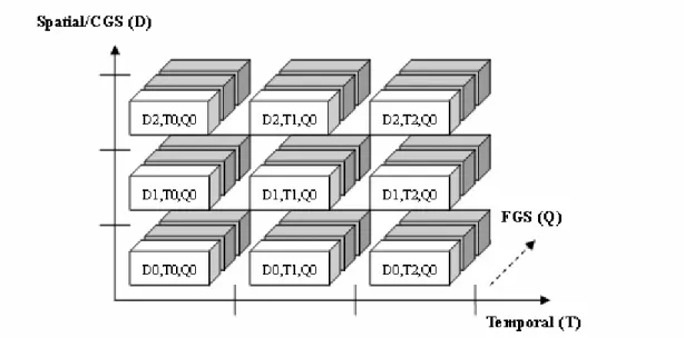
In this article, we define the term sub-layer as a set of NAL units with the same values of dependency_id (D), temporal_level (T) and quality_level (Q). Figure 11 depicts a three-dimensional sub-layer representation of a fully scalable bit-stream. Each cube represents a sub-layer.

Figure 11: Sub-layer representation

Since the coded data each sub-layer must be completely received in order to decode (expect for FGS), we consider sub-layers as the basic unit for extraction. For simplicity, we currently do not consider FGS.

3.1.3 Coding Dependencies

To ensure that an extracted bit-stream can be completely decoded, the coding dependencies must be satisfied. In SVC, the coded data consists of two types of coding dependencies:

„ Temporal Dependency

Temporal dependency is determined by the motion-compensated prediction between video frames. Using the hierarchical-B prediction structure, pictures of the temporal level k depends on pictures of temporal level k-1.

„ Inter-layer Dependency

Inter-layer dependency is determined by the inter-layer prediction between the spatial and SNR layers. A typical configuration is to let each layer k depend on layer k-1.

Combined Prediction Structure

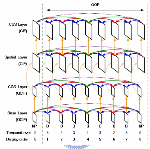
Figure 12 depicts an example of a prediction structure for combined scalability with a GOP size of 8. The bit-stream contains four layers: (1) a base layer for QCIF (176x144) resolution, (2) an SNR layer for QCIF resolution, (3) a spatial layer for CIF (352x288) resolution, and (4) an SNR layer for CIF resolution. Every layer is provided with four temporal levels. In this example, a total of 16 spatial, temporal and SNR resolutions are supported. The pictures are predicted as illustrated.

Figure 12: Prediction structure for combined scalability

Sub-layer Representation with Prediction Arrows

We illustrate the encoded bit-stream of the above prediction structure using the sub-layer representation with prediction arrows, as shown in Figure 13. Note that the values of quality_level are not considered since FGS is not used. Temporal dependencies are illustrated with the horizontal prediction arrows. Inter-layer dependencies are illustrated with the vertical prediction arrows.

Figure 13: Sub-layer representation with prediction arrows

Required Sub-layers

By traversing the prediction arrows in Figure 13, we can find out which sub-sets of sub-layers are required for decoding at each resolution. For example, to achieve the maximum resolution CIF_SNR@30, the corresponding sub-layer (D3, T3) needs to be decoded. The sub-layer (D3, T3) is predicted by (D3, T2) and (D2, T3). Nevertheless, (D3, T2) and (D2, T3) are predicted by other sub-layers. Recursively, we find that all 16 sub-layers are required for decoding (D3, T3).

If the target resolution is CIF@30, the bit-stream extractor extracts all NAL units with a dependency_id value lower than 3. Thus, a total of 12 sub-layers are required. If the target resolution is [email protected], the bit-stream extractor extracts all NAL units with a temporal_level value lower than 2. Thus a total of 8 sub-layers are required. Table 1 shows the required dependency_id and temporal_level of the necessary NAL units for decoding at each spatial, temporal and SNR resolution.

Table 1: Required sub-layers for different resolutions

Resolution Required D(s) Required T(s) Total sub-layers

[email protected] 0 0 1 [email protected] 0 0, 1 2 QCIF@15 0 0, 1, 2 3 QCIF@30 0 0, 1, 2, 3 4 [email protected] 0, 1 0 2 [email protected] 0, 1 0, 1 4 QCIF_SNR@15 0, 1 0, 1, 2 6 QCIF_SNR@30 0, 1 0, 1, 2, 3 8 [email protected] 0, 1, 2 0 3 [email protected] 0, 1, 2 0, 1 6 CIF@15 0, 1, 2 0, 1, 2 9 CIF@30 0, 1, 2 0, 1, 2, 3 12 [email protected] 0, 1, 2, 3 0 4 [email protected] 0, 1, 2, 3 0, 1 8 CIF_SNR@15 0, 1, 2, 3 0, 1, 2 12 CIF_SNR@30 0, 1, 2, 3 0, 1, 2, 3 16 Incomplete Bit-streams

For a target resolution, if any of the required sub-layers are missing, the bit-stream can not be properly decoded (without error concealment) at that resolution. We call this an incomplete bit-stream. However, the incomplete bit-stream can still be decoded at a reduced target resolution, if the coding dependencies of the reduced resolution can be satisfied.

Figure 14 depicts an example of an incomplete bit-stream with a missing sub-layer. In the example, the target resolution is [email protected], but a required sub-layer (D1, T1) is missing. Since the bit-stream contains (D0, T0), (D0, T1) and (D1, T0), the bit-stream can still decode at either [email protected] or [email protected]. However, either (D1, T0) or (D0, T1) is unused.

Figure 14: Incomplete bit-stream with a missing sub-layer (D1, T1)

Now if the decoder does provide error concealment techniques, it is possible to decode incomplete bit-streams at the target resolution even with missing data. However, frame loss concealment is non-normative and is currently only supported for bit-streams that provide two-layer spatial scalability in the JSVM software. Therefore, we will not consider error concealment.

3.2 Path Permutation

Given the coding dependencies, our next step is to find all the possible extraction paths. Extraction paths that violate the coding order (or dependencies) will cause a large portion of the extracted bit-stream not decodable. These bit-streams clearly cause inefficiency of bit-rate, therefore are considered as invalid

extraction paths. In this section, we will present two concepts for valid path permutation, namely wavefront sets and convex sets.

Valid Extraction Paths

Suppose a sub-layer B is predicted from a sub-layer A. If we extract sub-layer B before sub-layer A, then sub-layer B can not be decoded because sub-layer A is not provided. Oppositely, if we extract sub-layer A before sub-layer B, then sub-layer A is possibly decodable, as long as the depended sub-layers of A are also provided. In other words, extracting sub-layer B without sub-layer A can not improve the video quality but will only waste bit-rate. Given this reason, if sub-layer B depends on A, a valid extraction path should always extract A before B. If the coding dependencies of the extracted sub-layers are not satisfied, the extraction path is invalid.

3.2.1 Wavefront Sets

The concept of wavefront sets is to allow incomplete bit-streams, as long as not violating the coding dependencies. Figure 15 depicts an example of an extraction path using wavefront sets. Starting from the base sub-layer, each sub-layer is extracted one by one. The extraction order is like water flooding towards the destination at the other end. At each step, the extracted bit-stream may be incomplete, but the extraction path always remains valid. For example, after the second step, the extracted sub-layers are (D0, T0), (D0, T1) and (D1, T0). This is an incomplete bit-stream, but the coding dependencies of the three extracted sub-layers are satisfied. Therefore, this extraction path is still valid.

Figure 15: Extraction path using wavefront sets

The concept of wavefront sets allows a very thorough testing of valid extraction paths, especially for the case of error concealment allowed. However, the number of possible extraction paths becomes very large if the bit-stream contains a lot of sub-layers.

3.2.2 Convex Sets

The concept of convex sets is to always extract completely decodable bit-streams. Figure 16 depicts an example of an extraction path using convex sets. Starting from the base sub-layer, this extraction path increases the temporal resolution first, and then increases the SNR and spatial resolutions.

Figure 16: Extraction path using convex sets

Table 2 shows the extracted sub-layers for this extraction path. Note that each step in the extraction paths may extract more than one sub-layer, due to fulfilling the coding dependencies. For example, extraction step #4 adds four sub-layers for moving from QCIF@30 to QCIF_SNR@30. This is because the sub-layers with dependency_id value of 1 and temporal_level value of 0, 1, 2 and 3 are added in order to decode the sub-layer (D1, T3).

Table 2: Extracted sub-layers

Step Resolution Extracted D(s) Extracted T(s) Added sub-layers

#0 [email protected] 0 0 (0,0) #1 [email protected] 0 0, 1 (0,1) #2 QCIF@15 0 0, 1, 2 (0,2) #3 QCIF@30 0 0, 1, 2, 3 (0,3) #4 QCIF_SNR@30 0, 1 0, 1, 2, 3 (1,0),(1,1),(1,2),(1,3) #5 CIF@30 0, 1, 2 0, 1, 2, 3 (2,0),(2,1),(2,2),(2,3) #6 CIF_SNR@30 0, 1, 2, 3 0, 1, 2, 3 (3,0),(3,1),(3,2),(3,3)

3.3 Path Optimization

The main goal of this work is to find the optimal extraction path, such that the bit-stream data is extracted to maximize the decoded video quality subject to the bit-rate constraint. Due to the unequal size and unequal importance of each sub-layer in SVC bit-streams, we expect that different extraction paths should result in different rate-distortion performances. We evaluate the overall performance of each extraction path using the rate-distortion curves.

Rate-distortion Curves

Suppose that the bit-stream contains a total of 4 sub-layers (A, B, C and D), while sub-layers B and C are independent of each other. Different orders of extracting sub-layers B and C may show different impacts on the distortion. Figure 17 depicts an example of the rate-distortion curves of two valid extraction paths.

Figure 17: Example of rate-distortion curves

Lower distortion values indicate better playback quality of the decoded video. As more sub-layers are added to the extracted bit-stream, the rate increases while the distortion decreases. In this example, the distortion of the extraction path #1 is lower than or equal to extraction path #2 at any bit-rate. Therefore, the extraction path #1 is clearly the optimal in a rate-distortion sense.

the other extraction path for all bit-rates, we propose two optimization methods for determining the better extraction path. Figure 18 depicts an example of the rate-distortion curves showing this situation.

Figure 18: Another example of rate-distortion curves

3.3.1 Global Optimal

The global optimization of extraction paths is based on the convexity of the rate-distortion curves. The R-D curve that is closest to convex hull means that the distortion decreases as quickly as possible while the rate increases. The global optimal method is based on an exhaustive search in all possible extraction paths.

For each extraction path, the rate and distortion values are measured. Then we calculate the integral below the rate-distortion curve in the range of minimum and maximum supported bit-rate, depicted in Figure 19. The extraction path with the smallest area is chosen as the global optimal, meaning that the distortion decreases quickly while the rate increases.

3.3.2 Local Optimal

The local optimization of extraction paths is based on the rate-distortion slope of each sub-layer. The idea is to build the extraction path incrementally, starting from the minimum bit-rate and then choosing the next sub-layer to add into extracted bit-stream. For each step, the sub-layer with largest slope is selected from the available sub-layers.

The slope of a sub-layer is defined as the delta distortion divided by delta rate. The delta rate value is the sum of all NAL unit sizes belonging to that sub-layer. The delta distortion is the difference of the measured distortion, of the reconstructed sequence with and without that sub-layer.

3.4 Distortion Measurement

Distortion is used to indicate the playback quality of the decoded video. We measure distortion by calculating the mean square error (MSE) of the reconstructed frames against the original frames.

FrameSize P P MSE FrameSize n n n 2 1 ) ' (

∑

= − = n

P is the value of the nth pixel of the original frame. is value of the nth pixel of the reconstructed frame. However, MSE does not perfectly reflect differences of the perceptual quality for different device types. Therefore, we propose to consider device simulation.

n

P'

3.4.1 Device Simulation

In order to simulate the perceptual playback quality of the reconstructed sequence on different target device types, we propose that distortion should be

measured at the actual spatio-temporal resolution of the playback device.

Spatial Rescaling

If the spatial resolution of the reconstructed sequence is lower than the screen size of the playback device, the reconstructed sequence is spatially up-sampled. This makes sense because the playback device usually up-samples the reconstructed frames to its screen size before display. If the spatial resolution of the reconstructed sequence is larger than the screen size of the playback device, which is not the usual case, the reconstructed sequence is spatially down-sampled.

Temporal Rescaling

In order to compare the perceptual playback quality of different frame rates, we measure distortion at the maximum supported frame rate of the playback device. If the temporal resolution of the reconstructed sequence is lower than the frame rate of the playback device, then the missing frames are concealed using the picture copy method. Picture copy simply duplicates the previous decoded picture in display order. This simulates a frame freezing effect, which is reasonable since most playback devices actually display the previous frame in buffer instead of displaying a black frame when the frame rate drops. The distortion for low frame rates will depend on the performance of picture copy.

3.5 Program Architecture

Figure 20 depicts the architecture of the proposed extraction path optimizer. The path permutation module generates all possible extraction paths according to the coding dependencies. The module contains a checking function that removes the invalid extraction paths (causing incomplete bit-streams). A rate limiter module controls the target bit-rate for extraction. The target bit-rate is incrementally raised to test all the decodable rate points for each extraction path. For each test condition,

the SVC extractor and SVC decoder produces the reconstructed sequence using the tested extraction path. A device simulation module rescales the decoded video signal to match the resolution of the target device type. Then, the rate-distortion curves are measured and stored. After testing all conditions, the optimizer evaluates the rate-distortion curves and searches for the optimal path. Given a list common device types, an optimal path for each device type is be selected, producing a list of optimal paths. The optimal paths are calculated for every GOP in the input SVC bit-stream. To reduce the amount of storage and signaling for optimal paths, averaged optimal paths can be calculated for a sequence of GOPs

3.6 Extraction Framework

Figure 21 depicts the conceptual framework of using optimal extraction paths for extraction. The SVC encoder is used to encode the global bit-stream. The extraction path optimizer analyzes the global bit-stream and finds the optimal extraction path for each generic device type. The optimizer outputs a list of optimal paths, one optimal path for each device type. The extractor performs bit-stream extraction according to the client’s device type and available bit-rate. The bit-rate of the extracted bit-stream is controlled not to exceed the client’s available bit-rate. Using the device-specific optimal path, the extractor extracts the rate-distortion optimized bit-stream for each client.

Figure 21: Framework for extraction using optimal paths

In this system, the encoder and optimizer process are only run once. The resulting global bit-stream and optimal path list can be distributed and stored on multiple servers. The extractors on each server can extract bit-streams on-the-fly to match each client’s capabilities.

Chapter 4 Experiments

4.1 System Configuration

For experiments, we use the JSVM 7.0 to encode the scalable bit-streams. Each bit-stream is encoded with three layers and a GOP size of 8. The encoder settings are configured as follows:

„ The first layer is the base layer for QCIF resolution with a quantization parameter (QP) = 32.

„ The second layer is the CGS layer for QCIF resolution with a QP = 26. „ The third layer is the spatial layer for CIF resolution with a QP = 32. „ Each layer is encoded with four temporal levels, supporting the frame

rates of 3.75 fps, 7.5 fps, 15 fps and 30 fps.

4.2 Experimental Method

We setup a series of experiments to observe the rate-distortion performances of bit-stream extraction with different extraction paths. We will compare the results of using different test sequences and different target device types.

Our testing conditions are configured as follows:

„ Four test sequences are used as input data, including Akiyo, Foreman, Football and Mobile.

„ Four target device types are emulated in the extraction path optimizer, including CIF30, CIF15, QCIF30 and QCIF15.

„ For each test case, both the local optimal and global optimal methods are used to optimize extraction paths.

(allow incomplete bit-streams) and convex sets (always extract completely decodable bit-streams).

4.3 Results and Analysis

4.3.1 Comparison of Extraction Paths

As previously mentioned, we expect that different extraction paths should result in different rate-distortion performances due to the unequal size and unequal importance of each sub-layer in SVC bit-streams. To verify this assumption, we run several tests using the exact same test sequence and target device, but with different extraction paths.

Figure 22 shows the two different extraction paths. Path #1 starts with extracting the QCIF base layer and QCIF SNR layer and while increasing the frame rate to 15 fps. Then the CIF spatial layer is extracted. Path #2 extracts the QCIF base layer, the QCIF SNR layer and the CIF spatial layer while increasing the frame rate. At low bit-rates, path #2 will extract high resolution frames but with a very low frame rate. Path #1 will extract lower resolution frames but with a higher frame rate.

We compare the results of these two different extraction paths for playing the Akiyo sequence on a QCIF15 device. We plot the rate-distortion curves of each extraction path in Figure 23, where the y-axis represents the average MSE of all frames in a GOP and the x-axis represents the cumulative data size of the extracted sub-layers in a GOP for each extraction step.

Figure 23: R-D curve for different extraction paths

From the R-D curves, we can observe that the measured distortion for each extraction path is different at certain rates. When the rate is at 4000 bits, the distortion for the path #1 is lower than path #2. The path #1 has smaller area below the R-D curve and is more optimal than path #2.

4.3.2 Comparison of Device Types

Now, we compare the rate-distortion performances of the optimal extraction paths on difference device types using the same test sequences. For the Foreman sequence, the optimal extraction paths for the device types QCIF15 and QCIF30 are shown in Figure 24. The results show that the optimal extraction paths for different

device types do differ.

Figure 24: Optimal extraction paths for QCIF15 and QCIF30

For a QCIF15 device, the optimal extraction path starts with increasing the temporal_level until a value of 2. Then it starts to increase the dependency_id. Lastly, the temporal_level is increased to 3. For a QCIF30 device, the optimal extraction path increases the temporal_level to the maximum value and then increases the dependency_id. Comparing the third extraction step, SNR enhancement is chosen for a QCIF15 device while temporal enhancement for 30 fps is chosen for a QCIF30 device.

Figure 25 shows the R-D curve of the optimal path for the Foreman sequence on a QCIF15 device. Notice that no improvement in distortion is observed for the last extraction step, which corresponds to increasing the value of temporal_level to 3. This reflects the fact that a QCIF15 device does not need the temporal enhancement for 30 fps, since the device cannot display at such a high frame rate.

Figure 25: R-D curve for QCIF15

4.3.3 Comparison of Test Sequences

We compare the results of different test sequences, using the same device type. Figure 26 shows the optimal extraction paths of the Akiyo and Foreman sequence, both playing on a CIF30 device.

Figure 26: Optimal extraction paths for Akiyo and Foreman

We observe that the optimal extraction paths for the two test sequences are very different. For the Akiyo sequence, the dependency_id is increased to the maximum

value first. For the Foreman sequence, the temporal_level is increased to the maximum value first. These two sequences show completely opposite preferences of extraction. This hints that the selection of optimal extraction paths is affected by the characteristics of the content.

The content of the Akiyo sequence is a female reporting the news, which shows almost no movement except for some facial expressions. When the sequence is very static, the visual difference between high and low frame rates is not significant. Therefore, increasing the frame rate is not as important as increasing the SNR or spatial resolution for the Akiyo sequence.

The content of the Foreman sequence is a worker talking energetically while the camera is a little bit shaking. When the sequence is dynamic, the visual difference between high and low frame rates is significant. Therefore, increasing the frame rate is more important than increasing the SNR or spatial resolution for the Foreman sequence.

4.3.4 Comparison of Wavefront and Convex Sets

We have mentioned that incomplete bit-streams should result in poor performance since the bit-stream contains sub-layers that are not decodable. Convex sets do not allow extraction steps that will extract incomplete bit-streams. Wavefront sets allow extracting incomplete bit-streams. The client may make use of the incomplete bit-streams by simulated error concealment.

Figure 27 and Figure 28 shows two test cases of using convex sets and wavefront sets. Note that the extraction path of the wavefront sets has as much steps as the total number of sub-layers, such that each step adds exactly one sub-layer. The comparison results show that the global optimal path of using convex sets always follows the global optimal path of using wavefront sets, although using fewer

extraction steps. From this result, we believe that it is not necessary to use wavefront sets when considering global optimal extraction paths.

Figure 27: Results of convex and wavefront sets for Akiyo on QCIF30

Figure 28: Results of convex and wavefront sets for Foreman on QCIF30

4.3.5 Comparison of Global and Local Optimal

paths. Interestingly, when using convex sets for path permutation, all of the local optimal paths are the same as the global optimal paths.

When using wavefront sets, some cases show different results. Figure 29 shows an example of a local optimal path that differs from the global optimal path. Comparing the second step of both extraction paths, we observe that local optimal chooses a larger R-D slop than global optimal, which sounds like the better choice. However, the distortion of global optimal quickly decreases after the third step. Local optimization may lead to worse results than global optimization, since local optimization only considers the next step when building the extraction path, while global optimization performs an exhaustive search. Nevertheless, local optimal paths perform as good as global optimal paths when considering convex sets, which we believe is the practical situation.

Figure 29: Comparison of local and global optimal paths

4.3.6 Deduction of Optimal Paths for Different Devices

paths for different devices. For devices with the same spatial resolution, the optimal paths for 15 fps are similar to the optimal paths for 30 fps, except for the extraction of temporal enhancement for 30 fps. In these results, we suspect that by optimizing for the device with maximum frame rate, we can deduce the optimal paths for other device with lower frame rates. In Figure 30, the optimal path for QCIF15 can be deduced from the optimal path for QCIF30 by moving the extraction order of the temporal enhancement for 30 fps to the last extraction step.

Figure 30: Deduce 15 fps from 30 fps

4.3.7 R-D Performance of Sub-layers

The R-D performance of sub-layer can be understood as the impact of a sub-layer to the rate and distortion at the client. We evaluate this impact as the improvement of distortion divided by the increase of rate.

Figure 31 shows the R-D curve of the optimal path for the Akiyo sequence on a QCIF15 device. The yellow bars indicate the R-D performance of each extraction step. Each step may represent extracting one or more sub-layers. As shown, the

values for steps 1 ~ 4 are positive but decreasing, which means the extracted sub-layers at each step have decreasing amounts of good effect on the reconstructed frames. Note that for the last step, the importance for sub-layers with temporal_level values of 3 is zero. As mentioned before, this is because the QCIF15 device cannot display at 30 fps.

Figure 31: R-D curve of Akiyo on QCIF15

Figure 32 shows the R-D curve of the optimal path for the Foreman sequence on a CIF30 device. We specifically point out the fourth extraction step, where the rate is around 60000 bits. This step represents extracting all sub-layers with a dependency_id value of 1, which is the QCIF SNR layer. Note that the R-D performance of this step is very low, even lower than the last step. We can guess that the SNR enhancement for QCIF resolution is not very helpful for playback on a CIF30 device. But why is it extracted before the last step, which has a better R-D performance?

The R-D performance of CIF spatial layer is actually dependent of the QCIF SNR layer. This is because the QCIF SNR layer is required in order to decode the

CIF spatial layer. Without the QCIF SNR layer, the R-D performance of the CIF spatial layer would be zero. Therefore, the values of R-D performance of each step in an optimal path are not always ordered in a decreasing manner, some required sub-layers must be extracted first to satisfy the coding dependencies.

Chapter 5 Multisource Streaming

5.1 Introduction

The considered transmission scenario is video streaming in a network consisting of multiple servers and multiple clients, as depicted in Figure 33. Using multiple servers help to provide a higher overall throughput while allowing clients to retrieve data from diverse paths and servers, thus amortizes the network load. In this network, each node may act as a client and a server at the same time. In fact, a single physical node may act as multiple virtual servers at the same time, each virtual server providing different streams.

Figure 33: Multiple servers and multiple clients

To provide expandability, a large amount of servers are required in such systems. Using peer-to-peer overlay, each network node joining the service is utilized as a virtual server to help relay the video streams. Due to the heterogeneity of network bandwidths, each server may provide different amounts of dedicated bandwidth for the streaming service. Depending on the requested data of each

network node, each server may provide different sub-sets of sub-layers. Note that there is no synchronization among servers. Each server schedules and transmits video streams independently.

On the other hand, a larger amount of clients consume these server resources. The user device types may differ for each client while the amount of clients is time-varying. The clients may have different requests of video data. The total request rates of all clients may even exceed the provided server bandwidths. How to utilize the limited resources of clients and servers to provide optimal video streaming is a major issue. The transmission scenario is depicted in Figure 34.

Figure 34: Transmission scenario

For SVC-based multisource streaming, we propose a client-server scheme for bandwidth allocation. We suppose that optimal extraction paths are known to servers and clients. When a client suffers poor bandwidth or high packet loss rate, receiving all the layers is no longer possible due to the client’s limited throughput. In our system, clients have control over the requested rate of each layer. In other words, clients are allowed to selected the set of requested layers and determine the rate of

each layer. Given the rate-distortion optimized extraction path, clients can perform layer selection that is optimal for its device type under different bit-rates.

We will focus on the bandwidth request and allocation strategies of the client and the server.

5.2 Coding Scheme

Rateless Codes

Erasure correcting codes are commonly applied to video transmission over lossy channels to avoid retransmissions. Fountain codes [10], or rateless codes, are erasure correcting codes that have the following properties:

„ Allows generating unlimited number of encoding symbols, without predetermined coding rates.

„ Allows independent generation of each encoding symbol using separate encoders.

„ Any k (1+є) of the encoding symbols can be used by the decoder to reconstruct the original k source symbols.

The concept of receiving fountain encoded data relates to filling a glass of water from a fountain. Once the glass is full, the data is received, no matter which specific water drop is obtained. The water may even be obtained at different fountains, as long as the input source symbols are the same.

Combining Video and Channel Coding

In our multisource streaming scheme, we propose to send SVC video data encoded with rateless erasure correction codes. In SVC, multiple sub-layers are coded per GOP as depicted in Figure 35. We encode each sub-layer of each GOP separately to allow independent subscription of sub-layers according to client

preferences.

Figure 35: Multiple layers are coded per GOP

Figure 36 depicts the coding scheme of applying rateless codes to SVC. For each coded sub-layer per GOP, unlimited encoding symbols are distributed on multiple servers, while the client only needs to receive any k (1+є) of them.

Figure 36: Scalable video coding with rateless channel coding

This coding scheme gives us two important properties: „ Feasible server decentralization

Since rateless codes allow independent generation of encoding symbols, multiple servers can provide unlimited symbols on-the-fly. Most importantly, no coordination between servers is needed to prevent duplicated packets. Every encoding symbol is unique.

„ Flexible erasure protection

Serving multiple clients in heterogeneous networks requires dealing with unpredictable packet losses. A robust video transmission system not only needs to adapt to channel-specific bandwidth and loss rates but also provide device-specific unequal layer protection. Using traditional erasure codes, such requirements would require adjusting the coding rate. Using rateless codes, such resiliency scalability is achieved by adjusting the number of encoding symbols sent.

5.3 Negotiation Protocol

The proposed bandwidth allocation is based on a three-way negotiation protocol between each client-server pair. This application layer negotiation protocol has three types of control signals, namely REQUEST, REPLY and CONFIRM.

„ REQUEST

This signal is sent from the client to the server. The client specifies a list of requested layers and the requested bit-rates corresponding to each layer. „ REPLY

This signal is sent from the server to the client. The server specifies a list of reserved layers and the reserved bit-rates corresponding to each layer. The values of reserved bit-rates depend on the availability of the server’s bandwidth, ranging from zero (completely denied) to the client’s requested bit-rate (completely accepted).

„ CONFIRM

This signal is sent from the client to the server. The client specifies a list of reserved layers and a final confirmation to the server. The signal may be an ACK or a NACK, depending on the client’s allocation strategy.

Figure 37 depicts an example of the negotiation protocol of one client and two servers. The server provides reserved bandwidths to clients for durations in terms of GOPs, called sessions. Before every session, the client determines the requested servers and the corresponding requested rates for the next session. In each negotiation round, the client first sends the REQUEST signals to all requested servers. Note that clients may ask more requested servers than required. The servers may also receive requests from one or more clients during its decision time window. The server determines the reserved rates for each requesting client and sends a REPLY signal to each requesting client. The client must send a CONFIRM signal back to the server to acknowledge the reservation, or else the server will release the reserved bandwidth. The client will determine from the received REPLY signals whether more servers need to be requested.

Figure 37: Negotiation Protocol

5.4 Server Scheme

Each server multicasts video streams to the clients according to its own time. We assume that explicit time markers of video data are available to servers (similar to RTP timestamps, for example). No synchronization between servers are assumed nor required. Different servers may be multicasting different GOPs at the same moment, but we assume that client buffers are capable of aligning the received data

according to explicit GOP markers.

We have a system-wide parameter called RateStepSize, which refers to the minimum reserved rate per request. Such a setting is to simplify the management of rate allocation, though may be extended to be a server-dependent parameter in the future. For a server with a dedicated server bandwidth of Rs, the server provides as

many as (Rs / RateStepSize) user slots per session. Client requests will try to fill in

unoccupied slots for the next session. For each accepted client, the server will reserve bandwidth of the next session for the client. However, when the total request rate exceeds the server available bandwidth, the server must deny some of the requests, starting from the relatively unimportant requests. This may result in accepting a portion of a client’s request while denying the other portion.

For fairness, client requests are prioritized according to layer priorities for the device type of the client. A decision time window at the server will allow multiple clients that requested during the duration to be compared at once. The server allocation refreshes each session, thus clients are responsible to actively subscribe for resources every session.

5.5 Client Scheme

Figure 38 depicts the client scheme of our proposed protocol. There are two levels of client updates, namely service update and session update. Service update is to fetch the server list from the P2P overlay (provided by DHT or tracker, for example), normally once per 15 minutes. The server list specifies the network address and dedicated service bandwidth of each server. Each server may contain different layers, so the served layers of each server are also specified. Session updates are triggered every session, normally once per 30 seconds. The server list is not fetched each session. The actual loss rates of connected servers are recorded

after each session.

Figure 38: Client Scheme

The client algorithm includes the rate allocation method and server selection method. The rate allocation method determines the total requested rate of each sub-layer. The server selection method determines which servers to request for each sub-layer. Multiple negotiation rounds are needed if some requests are not accepted. For such cases, the server selection method picks other servers for each round. If the session is about to begin and there is no more negotiation time, the client will try to request the next session. In the following sections, we will introduce the client algorithms.

5.5.1 Rate Allocation

The rate allocation method determines the total requested rate r(layer ID)of each sub-layer using the following equations:

(

)

GOPsize te MaxFrameRa T l x e k l r _l ⋅ _D ⋅ _l⋅ − ⋅ + ⋅ = ( ) 1 1 1 ) ( ε

The parameters include the data length kl, coding overhead ε, symbol size Tl,

actual loss rate e and layer protection factor xD(l). The coding overhead and symbol

size are the encoding settings for erasure correction coding. The actual loss rate is obtained from connection records, initially zero before transmission. The layer protection factor xD(l) represents the unequal importance of each layer, and specifies

a different amount of error correction redundancy. The essential parts of the requested rate is k_l ⋅ 1

(

+ε

)

while the redundant parts of the requested rate is

) ( 1 1 l x e⋅ D − .

The layer protection factor for device type D and layer l is calculated according to the layer priorities PD(l). The important layers are encoded with extra redundancy

while the most unimportant layer is encoded with no redundancy. The values of xD

are in the range of 1.0 and 2.0. We use a heuristic solution as the following equation: ) 1 ) ( 1 ( ) ( − − + = MaxP l P MaxP l x D D

After the total requested rate is calculated, the value of r(l) is rounded to the next “rate step”. Such rate quantization simplifies the management of server bandwidth reservation. ze RateStepSi ze RateStepSi l r l r _⎥⋅ ⎥ ⎤ ⎢ ⎢ ⎡ = ( ) ) ( '

Once the quantized request rate for each layer is determined, the next step is to select the requested layers according to client bandwidth. If not enough bandwidth is available, the client will request the most important layers first (with lowest layer priority values).

Each layer will be requested from multiple servers, therefore the requested rate per server depends on the number of requested servers. To amortize network load,