泛用型動態虛擬實境操控與運動復健輔助系統研發(III)---子計畫I：動態VR運動復健輔助系統之行為轉換與即時模擬研究

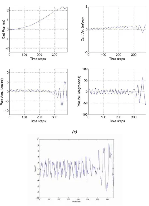
行政院國家科學委員會補助專題研究計畫

▓ 成 果 報 告

□期中進度報告

泛用型動態虛擬實境操控與運動復健輔助系統研發



子計畫 一：動態 VR 運動復健輔助系統之行為轉換與即時模擬研究

計畫類別：□ 個別型計畫 ▓ 整合型計畫

計畫編號：

NSC92-2213-E-009-016

執行期間： 90 年 8 月 1 日 至 93 年 7 月 31 日

計畫主持人：李祖添 講座

教授

共同主持人：

蘇順豐 教授

計畫參與人員：

陳松雄、張原彰、陳政達、王彥評、林君彥、游雅婷、

李世翔、劉家和、張富傑、李明橋

成果報告類型(依經費核定清單規定繳交)：□精簡報告 ▓完整報告

本成果報告包括以下應繳交之附件：

□赴國外出差或研習心得報告一份

□赴大陸地區出差或研習心得報告一份

□出席國際學術會議心得報告及發表之論文各一份

□國際合作研究計畫國外研究報告書一份

處理方式：除產學合作研究計畫、提升產業技術及人才培育研究計畫、

列管計畫及下列情形者外，得立即公開查詢

□涉及專利或其他智慧財產權，□一年□二年後可公開查詢

執行單位：國立交通大學

中 華 民 國 93 年 7 月 日

泛用型動態虛擬實境操控與運動復健輔助系統研發



子計畫

一：動態 VR 運動復健輔助系統之行為轉換與即時模擬研究

計畫編號: NSC90-2213-E-009-104; NSC91-2213-E-009-036; 執行期限:90/08/01 - 93/07/31 主持人: 李祖添 講座教授; 共同主持人: 蘇順豐 教授 參與人員：陳松雄、張原彰、陳政達、王彥評、林君彥、游雅婷、李世翔、劉家和、 張富傑 國立交通大學電機與控制系、國立臺灣科技大學電機系 一、計畫概述 在本計畫研發的系統中，操控員透過操控界面下達指令，以操控系統中的虛擬的運動 訓練的輔助設備或載具。此操控命令將被輸入所模擬之設備或載具的精確物理模型中，以 求得真實情況下系統的反應(包括姿態、速度、加速度、力道等)。這些反應將透過本子計 畫的行為轉換與控制模組，而由六軸運動平台、力迴饋模組(Force feedback)及虛擬實境顯 示器表現出來，以讓操控員獲得身歷其境的感受。這整個系統中，因為行為轉換模組的設 計扮演實際環境裡物體運動狀況以及虛擬環境中操控員身體感受之間橋樑，如何讓操控員 有身歷其境的感受，有賴於在動態模擬系統發展過程中，適當的人(操控員)機(動態模擬器) 溝通界面及迴饋學習技術，以獲得最符合人類感覺的行為轉換模式。 在虛擬實境的運動訓練的輔助動態模擬系統中，當虛擬系統接收到控制命令，而設法 產生應有的運動行為描述時，在虛擬實境的顯示以及在模擬運動平台的運動行為，則是要 儘可能地模擬並使其有身歷其境的感受，以達到虛擬實境的目的。文獻上之動態模擬有固 定平台及動作平台二類，動作平台大部分是在飛機模擬用，動作平台之動作方式若不符合 真實情形，比不用還要糟糕。而為了達到此一目標，上述的運動行為描述必須恰當的轉換 給虛擬實境運動平台的控制系統。對虛擬實境的顯示而言，由於在顯示部分其為一動畫系 統；並在理想上，將盡可能的和真實系統貼近，而且所有之運動行為都是以顯示的方式來 呈現，並且由於虛擬實境的顯示的產生是可以由系統再修正，因此在運動行為的呈現上較 容易。因此，本子計畫只要將相關之運動行為提供給顯示子系統即可。Stewart Platform 為 一具有六自由度運動能力之機械平台，但其運動範圍受到其工作空間的限制，有些動作是 無法達成的，因此為了在其有限空間下模擬出騎馬、飛機、輪船等交通工具時之運動感覺。 所以一般是以沖淡演算法(Washout Algorithm)架構出對模擬器的力的感受。 本子計畫主要在於建立所欲模擬之場景及運動項目的精確物理模型，以便當接受子計 畫三所傳送之使用者操控指令時，能精確獲得被模擬之運動項目在真實環境下的反應，而 經由行為轉換與控制送至子計畫二，在虛擬實境中展現出來。因此本子計畫相當於整個動 態虛擬實境運動復健輔助系統的輸入單元。在本研究中，由於真實系統並不是在旁邊實際 動作，因此如何真實地精細架構真實系統之模式，以產生逼真的系統反應行為於虛擬實境 的動態模擬器中，便是個非常重要的課題。同時由於希望能更精確的反應出行為來，傳統 的模式建立可能無法達成如此精確的要求，因此本子計畫將研究如何地綜合利用物理運動 定律，輸出、入行為，以及利用子計畫五之技術所擷取的人為修正訊息等，來精確地架構 出真實系統模式。本子計畫的另一個研究主題為如何將真實系統之運動行為轉換成模擬器 的控制命令，以及如何將無限空間中之運動感受，轉換成有限空間中運動的感受（如在加 速度前進所感受之反作用等）。因此本子計畫扮演本計畫中真實世界與虛擬世界的橋樑，它 將接受即時模擬單元來的行為狀態，再參考子計畫二所提供的六軸動作平台姿態訊息，以 及子計畫二、五所感測的使用者運動狀況資訊後，對子計畫二、三、四發出高階的控制命 令，以便使用者可以感受運動項目的姿態變化、力迴饋及場景更新。在模擬系統建立過程 中，本子計畫也將接受經由子計畫五來的使用者感受反應而調整其行為轉換及控制方式。

二、沖淡演算法級行為轉換演算法

本子計畫主要在於當虛擬系統接收到控制命令，設法產生應有的運動行為描述以及在 模擬運動平台的運動行為，以達到虛擬實境的目的。目前文獻上對於如是的轉換是以 Washout 演算法或稱 Washout Filter 的方式來設計[1-15]。Washout Filter 的輸入為由數學運 動模型所求得的比例力與角速度。所謂的比例力(Specific Force)是指單位質量所受的非重力 力。由向量的觀點來看的話，比例力即是慣性加速度與重力加速度之差，因此比例力可定 義為 fv =av−gv。此比例力的觀念在航太工程中被廣泛的使用，主要的應用是判斷飛行員在 飛行過程中是否會遭遇過大的比例力而飛生不可預期的危險，以及飛行載具的機械結構是 否足以承受。 在這裡，我們將完整介紹沖淡演算法的架構以及它在整個系統裡所扮演的角色。目前 實現沖淡演算法的方法很多，在此我們是採用廣泛被使用的典型沖淡演算法(University of Toronto Classic Washout Algorithm, UTCWA) [10-12]。圖一為沖淡演算法的架構，我們將以 此架構將模擬器上之一參考點之運動感覺轉換為其在上平台對應點之運動。沖淡演算法其 實是一種概念，它主要是利用人類對感覺具有門檻值的特性，適當地將某些頻率成分的線 性運動或轉動運動加以濾除，並將持續的比例力感覺用緩慢轉動一傾斜角的方式來實現， 這個傾斜角所產生的轉動被控制在人類對轉動感覺的門檻值以下，操作員將不會有明顯的 感覺，以避免混淆原本的轉動運動的感受。 人類對轉動運動的感受主要是由來自半球管，而比例力則是來自內耳石。這裡人体運 動感覺模型的輸入為我們前面所介紹的比例力與角速度，並且各自獨立的處理與運作，而 得到新的人体真正感覺得到的力與轉動運動。人体對頻率為0.2 rad/sec~10 rad/sec 的角速度 的感覺極為敏銳，當角速度或角加速度較為低頻或為一常數時，感覺較為遲鈍；而對頻率 為0.2 rad/sec~2 rad/sec 的比例力的感覺也極佳，而對持續的加速度感覺則趨於零。沖淡演 算法正是利用人類此一特殊的感覺模型所架構出來的。根據上面所述，人体對比例力與角 速度之感覺類似一帶通濾波器，但我們在實做上為了將較人体感覺更高頻的部份表現出 圖 一

來，所以我們以高通濾波器來實現。在平移運動(Translation Motion Channel)的部份，將駕 駛員在模擬器的數學模型下，所推導出來的力經過運動學轉換成本身的受力，經過一個比 例及極限處理器，或稱為scale block。這個 scale block 的主要作用就跟人体運動感覺模型 中的非線性衰減器一樣，其理由是人類對在門檻值以下之比例力感覺較為遲鈍而將之省 略，如此可以避免平台之高頻震顫，同時亦可以調變值的大小，並限定此輸入的大小以免 超出平台的動作極限，使其值更適合平台。fv₁和ω₁為機身座標的作用力描述，而在washout filter 中，大部分都會將fv₁和ω₁轉為慣性座標上的描述(也就是做座標轉換乘以L_1s和T )。_s 如是的轉換會使在模擬運動時，較容易回歸原點。可是在慣性座標上，運動及轉動動作軸 間二者間有Coupling 的效應。而在早期的實驗研究中[12]，可以看出這些 Coupling 效應是 較可忽略的，比起使用機身座標所產生原點的偏移。將fv₁利用轉換矩陣L 轉置為慣性座_IS 標系的座標向量後加上重力加速度gv ，最後將之通過一個高通濾波器。此濾波器主要的功I 用是將比例力中較低頻的部份加以濾除，只保留高頻中人体所以感受得到的部份，且能使 平台在原點附近動作以免超過其工作空間，這也是我們使用沖淡演算法最主要的用意－確 保平台在其原點動作而不至超過其工作空間，並能在有限空間內模擬出人体對動作的感 受。接下來將濾波器的輸出值av_H經過兩次積分以得到我們所要的平台三個軸所對應的動作 姿態的值，這個值就是模擬操縱者在模擬器中的受力情形所對應的位移運動。而轉動運動 (Rotation Motion Channel)的動作跟平移運動是很類似的。這個角度是模擬操縱者在模擬器 中所受到的轉動運動所對應的角度，但輸入平台的角度還必須加上如下所要說明的斜傾座 標所產生的傾斜角。

而斜傾座標系(Tilt Coordinate Channel)的作用，主要是用來模擬低頻的受力情形。在 模擬器最難實現的模擬狀況之一，就是一段長時間持續加速的過程，因為平台沒有足夠的 空間來完成這個動作。但是對人体而言，我們能感受的到的也只有一開始加速時身体受到 慣性作用，及向後傾與結束加速時身体向前傾的兩種受力情形。而中間這段時間大多是沒 有感覺的。但是我們一般可以利用視覺上的效果，來使人認為目前是正在動作的，這個動 作就是斜傾座標系利用重力加速度在X-Y 平面上之分量所製造出來的效果。這就是傾斜座 標的作用，傾斜一個角度造成視覺上的假像，並利用重力加速度的分量來模擬低頻的比例 力 。 利 用 重 力 加 速 度 來 產 生 傾 斜 角 度 βv_L =[θ_x θ_y θ_{z ] ， 其 中}T _sin 1_{( )} g f_Ly x − = θ 、 ) ( sin 1 g f_Lx y − − = θ 、θ_z =0，而g⋅sin(θ_x)= f_Ly和g⋅sin(−θ_y)= f_Ly。再將斜傾座標所產生的βv_L 與轉動運動所產生的βv_SH兩向量合起來前，βv_L還需經過Rate Limit Block，這個 Rate Limit 最主要的用意是將βv_L限制在人体對轉動速度感受不到的角度內，使人身体無法察覺斜傾座 標所產生的轉動動作，避免影響轉動運動所產生的動作，而僅是視覺上的模擬。然而斜傾 角的改變速率限制上必須要有限制，以免操作者感受到此一斜傾行為。在斜傾角速率限制 上，一般為在pitch 方向為 13deg/s，在 roll 方向為 2deg/s。

圖二

在文獻中[7-9]也有提出調適式的 Washout filter 如圖二為一調適式之 Washout filter， 其概念是根據線上取得的資訊去調整 Filter 中的增益。其主要是將平台的運動和被模擬之 運動之間的差異及平台特性的考量來，架構出一性能指標。並經由一最佳化的運算，來找 出增益調適的法則,由於指標函數及增益間之關係複雜及即時的需要。一般都是以最陡下降 (steepest decent)法來產生。如欲追隨之運動已知，則也可利用最佳控制的概念，來直接尋 找最佳之線性filter [10,11]。此一調適演算法主要的功能，即是要減低錯誤動作方式及使平 台儘量維持在原點。而在如圖二的架構中,其斜傾處理的計算也有所改變。首先其所利用的 信號本身就不一樣。在調適式架中由於是針對慣性座標軸，因此有許多的運動的斜傾反應， 也進入角度運動環路中了。因此其在調適的考慮上也變得非常複雜[15]。因此在[15]中，作 者也是出以傳統 Washout filter 架構的調適 Filter。因此本計畫將嘗試在這些方面進行探討 的研究，就我們所要研究的輔助系統來探討不同的Washout 演算法在不同狀況下的效能評 估。

表一 平移運動之非線性衰減器之參數 平移運動之非線性衰減器之參數

X 軸 Y 軸 Z 軸 Threshold Value d_T (_m/sec2) _{0.17 0.17 0.25}

Slope k_T 0.5 0.5 0.5

表二 轉動運動之非線性衰減器之參數 轉動運動之非線性衰減器之參數

Roll Pitch Yaw

Threshold Value d_R sec) (deg/ 3.0 3.6 3.6 Slope k_R 0.5 0.5 0.5 表三 濾波器之參數 Transfer function of Filters 2 2 1 1 2 2 1 1 0 1 ) ( _{− −} − − + + + + = z a z a z b z b b z T

High-Pass Filter 1 High-Pass Filter 2 Low-Pass Filter 1

0

1 b 0 -1.9131 0.0030 2 b -0.0378 0.9565 0.0015 1 a -1.9187 -1.9112 -1.8890 2 a 0.9244 0.9150 0.8949 在目前交大的Washout Filter 的參數(針對汽車運動)的非線性衰減器的參數值列於下表 一、二、三中。而必需說明的一點是，這些值並非是絕對的，因為每個人對運動的感受程 度不同值就會不同，甚至當時的身体狀況、心理狀況與專心程度不同也會影響的這些值， 所以表中所列的值僅是參考。我們將以這些參數來當一初始研究的標的，並進而了解在不 同狀態下，washout 演算法的調變效果，及若以加強式學習調變參數時，其效能及可變化極 限的研究。 而在目前研究中，washout 演算法大部分都是以飛機飛行為主要考慮對象。飛行動作 平台主要功能是訓練駕駛員，因此針對 Washout 演算法的設計由於被模擬的飛機是不變 的，因此可透過不斷的調整及改變使其效果變好，而且由於飛行模擬必須考慮極大的操作 範圍，不過其範圍不會突然變動很大，有時候是以數個不同的Washout 演算法來設計。在 本計劃的研究中，由於是屬於地面上的運動，而且根據不同的需求及不同的狀態。因此如 何使Washout 演算法能在這些系統中仍適用，或必須做恰當的轉換是值得探討與學習的。 同時由於地面運動體的運動反應一般較快而多變，這是因為運動體的質量小，因此當施於 作用力時，其必然能產生較顯著的反應。因此在Washout 演算法的設計上也變得較困難。 由於運動轉換主要的著眼點是操作者感受的正確性，因此取得操作者的回饋來進行系統修 正變得相當重要。因此在本子計劃的研究中，也想將操作者的回饋信息用來修正運動轉換 的相關機制。 固定平台的虛擬實境主要是靠影像部分來達成，當運動為直線定速時，如是的模擬是 相當不錯的，可是當運動路徑是多變的時候，在轉彎加速或上下起伏時，在固定平台上的 感受就差很多。若使用動作平台時，由於虛擬系統能設法產生一些相對應的動作反應，使 操作者能感受到類似的感受力，此時在輔以影像的虛擬，確實能使虛擬實境達到更逼真的 效果。可是當動作平台產生誤動作時，整個系統的感受將是很不好的。因此如何去設計好 的動作，便是虛擬實境系統中不可或缺。此一部分的設計一般統稱為 motion cue。然而針 對motion cue 的設計，大致可分為兩類，其一為事先已知運動內容的，例如動態電影院或 虛擬歷險等，其所運動的路徑及方式都是事先已經設定好了。因此在實務上大多以經驗法 則加上現場測試調整來達成。另一類則是無法事先知道運動的內容，例如相關模擬操控系 統，其運動內容是由現場的命令來驅動的。因此無法以如上述的方式來設計 motion cue。 在飛機模擬系統中，大部分則是以前面所討論到的washout filter 來執行。在我們的研究中， 以上兩種行為轉換的motion cue 我們都將加以探討。在前者由於場景的設計及規劃大致其 運動範圍是固定的，而許多反應可能是來自於場景而非運動本身。因此我們將以運對動態 電影的分析來架構motion cue 的經驗法則。

Motion Simulation is to rebuild the feeling of passengers in a vehicle from a locally moving simulator. The most popular device utilized in motion simulation is Stewart platform. Stewart platform is a six-degree free device. Because Stewart platform is complicated and hard to design, washout filters are often used to fulfill motion simulation. The idea of washout filters is to ignore the frequency so that a limited workspace of platform can generate infinite motion. Originally, motion simulation is developed to train flight pilot. Nowadays, motion simulation not only is employed in flight simulation, but also can be used in various vehicle simulations. We design a spring device to be added after the washout filter to reduce the chance of reaching the boundary of the workspace.

The position of 6-degree free platform is defined by (x, y, z, roll, pitch, yaw). We divide it into two domains, the shift domain (x, y, z) and the angular domain (roll, pitch, yaw). Now we construct the relationship between each two vectors in each domain respectively. We now focus on the shift domain. Figs. 3~5 are the mutual relationships of each two vectors while other

variables are zero. The outer ellipses are the approximation field of the available field, and the inner ellipses are the safe zone. The fixed vector far away the origin the effective area is smaller. Hence, we can approximate the boundary of shift domain as an ellipsoid. The ellipsoid is described as 2 2 2 2 2 2 ( 15) 1 160 160 100 x ₊ y+ ₊ z _{= (1)}

The mutual relationships of each vector in the angular domain are shown in Figs. 6~8 while other variables are zero. The boundary of angular domain can also be approximate as an ellipsoid, and it is described as

2 2 2

2 2 2 1

15.8 16 15.2

roll ₊ pitch ₊ yaw _{= (2)}

-200 -150 -100 -50 0 50 100 150 200 -250 -200 -150 -100 -50 0 50 100 150 x y z=0

Fig. 3 The mutual relation between x and y with z=0.

-200 -150 -100 -50 0 50 100 150 200 -150 -100 -50 0 50 100 150 x z

-250 -200 -150 -100 -50 0 50 100 150 200 250 -150 -100 -50 0 50 100 150 y z

Fig. 5 The mutual relation between y and z with x=0.

-20 -15 -10 -5 0 5 10 15 20 -20 -15 -10 -5 0 5 10 15 20 roll pi tc h

Fig. 6 The mutual relation between roll and pitch with yaw=0.

-20 -15 -10 -5 0 5 10 15 20 -25 -20 -15 -10 -5 0 5 10 15 20 25 roll ya w Fig. 7 The mutual relation between roll and yaw with pitch=0.

-20 -15 -10 -5 0 5 10 15 20 -25 -20 -15 -10 -5 0 5 10 15 20 25 pitch ya w

Fig. 8 The mutual relation between pitch and yaw with roll=0.

We have defined the boundary of the working space and the warning zone and dangerous zone are described in Table 4.

Table 4 The equation of the working space surfaces. (x, y, z) (roll, pitch, yaw) Boundary Surface 2 2 2 2 2 2 ( 15) 1 160 160 100 x y+ z + + = 2_{2 2} 2 ₂2 1 15.8 16 15.2

roll pitch yaw

+ + = Warning Surface 2 2 2 2 2 2 ( 15) 1 80 80 50 x y+ z + + = ₂2 ₂ 2 ₂2 1 7.9 8 7.6

roll pitch yaw

+ + = Dangerous Surface 2 2 2 2 2 2 ( 15) 1 120 120 75 x y+ z + + = 2_{2 2} 2 2₂ 1 11.85 12 11.4

roll pitch yaw

+ + =

We consider a continuous acceleration motion. In Figs. 9 and 10, the solid line is the original position and the dash line is the position after spring device. We can see the dash line is very similar to the solid line. Thus, the feeling of pilot on the platform is very similar even the same. From Fig. 10, we can find that while the original trajectory is closer to the working space boundary, the new generated trajectory is changed bigger. In the other words, it is harder to move the actuators while the platform is closer to the working space boundary. In Fig. 10, we also can find the three still part of the original trajectory, the new generated trajectory moves slightly toward the original. In Fig. 11, the solid line is the original length of actuators and red dash line is the length of actuators after spring device. We can see the dash line is closer to origin than the solid line obviously.

Fig. 9 The displacement outputs after spring device.

Fig. 11 The length of actuators after spring device.

三、行為轉換演算法

在我們的國科會研究中，我們取得美新科技一組影片及對應的平台操控命令列，目前 我們在探討以資料庫的方式來建立的motion cue 的對應法則。有關 motion cue 方面，我們 也分析了一段雲霄飛車的影片，企圖來了解一般在motion cue 方面的設計概念。所得到的 心得如下：軸一主要操控上下的運動，而腳長縮短表示感受向上的力(加速度)，例如轉為 下坡運動的起始瞬間。而腳長伸長表示感受向下的力(加速度)，可分為兩種狀況，一是運 動轉為上波的瞬間，其二是一個下坡路段的盡頭，即轉為平地。軸二主要操控左右的運動， 而腳長縮短表示向左的力，例如右彎、右側的碰撞或路面右側高起。反之腳長伸長表示向 右的力，例如左彎、左側的碰撞或路面左側高起。軸三主要操控前後的運動，而腳長縮短 表示受到向後的力，例如加速。而腳長伸長表示受到向前的力，例如減速或是與前方物體 碰撞。軸四主要操控以平行車身為軸做旋轉的動作，而腳長伸長表示向左旋轉，例如路面 右側突起或是由左側突起路面轉為平地，也可用來輔助左彎。反之，腳長縮短表示向右旋 轉，例如路面左側突起或由右側突起路面轉為平地，也可輔助右彎。軸五主要操控以車身 的鉛直線為軸的旋轉運動，而腳長伸長代表逆時針旋轉，例如在左彎時。腳長縮短代表順 時針旋轉，例如右彎。軸六主要操控以左右方向為軸的旋轉運動，而腳長縮短代表往下旋 轉，例如路面轉為下坡或上坡結束。腳長伸長代表向上旋轉，例如轉為上坡或下坡結束。 另外直接以運動的觀點說明腳長的變化；加速為軸三縮短，軸六伸長。減速為軸三伸長， 軸六縮短。上坡為軸一伸長，軸六伸長。下坡為軸一縮短，軸六縮短。右彎為軸二縮短， 軸五縮短，若是傾斜路面軸四縮短。左彎為軸二伸長，軸五伸長，若是傾斜路面軸四伸長。 最後，我們觀察在這段影片中是否有偷偷把腳長拉回原點的動作。我並沒有發現有偷腳長 的現象，而是設計者以不超過平台運動範圍內任意設計，因此我們估計並不是每個類似動 作發生時乘坐在平台上的人員的感受強度都會一樣。可能發生在影片中這段的加速度比較 大但是感受卻比加速度比較小時來的強烈。也就是針對各種模擬主體的運動，我們將建立 其相對應的平台運動方式。

There is another way of dealing with the motion of simulators and is referred to as the motion cue. It is often used in the so-called virtual reality emulation theaters. Because this kind of application is an off-line system, engineers can design the platform variation to generate motion cues by their experience. Because of this property, there are two major advantages for motion cue. One is that because motion cue is an off-line mapping, we can plan the whole motion to avoid the

movement of actuators out of the working space. The other one is that special movements can be added to generate more entertaining effects. Because motion cue deeply relies on an experienced engineer to arrange a good motion cue trajectory of Stewart platform positions, we attempt to build fuzzy rules to make the motion cue design more easily. The performance of motion cue deeply depends upon the experience of the designer, and it can usually be designed delicately. The disadvantage of motion cue is that a well-designed motion cue always relies on engineers’ experience. Hence, we would like to discuss a method that engineers can plan motion cue easier even that the engineer is with less experience. Then, we focus on the trajectories of actuators. If we can find the relationships between motions and the length of actuators, we can easily design the motion cue without experience. Now we have a series of trajectory of length of actuators. We have found some relations between motions and length of actuators, and the main relations are described in Table 5.

Table 5 The relations between motions and actuators.

First Second Third Fourth Fifth Sixth

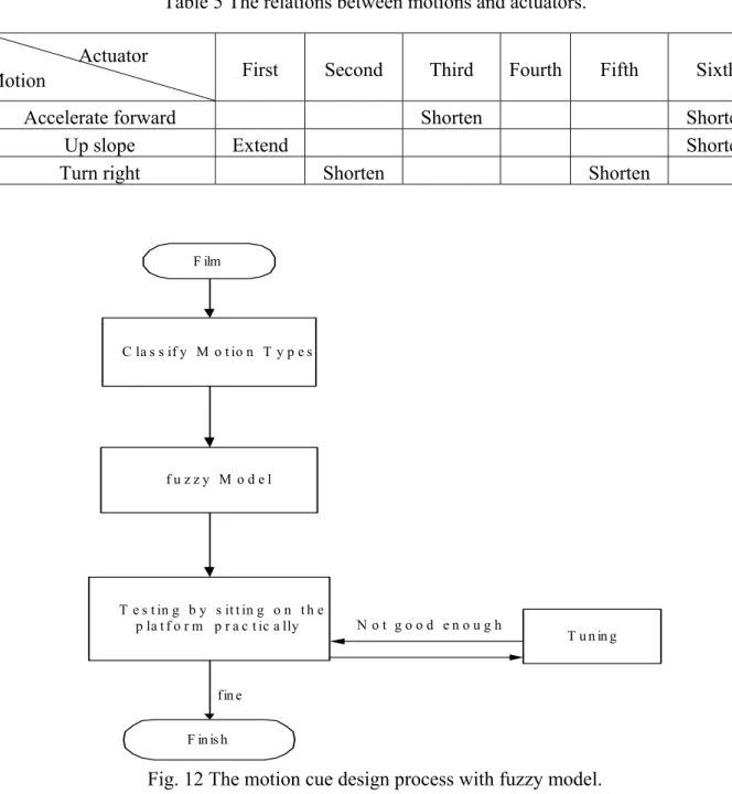
Accelerate forward Shorten Shorten Up slope Extend Shorten Turn right Shorten Shorten

F ilm C la s s if y M o t io n T y p e s T e s t in g b y s it t in g o n t h e p la t f o r m p r a c t ic a lly F in is h fin e T u n in g N o t g o o d e n o u g h f u z z y M o d e l

Fig. 12 The motion cue design process with fuzzy model.

Although we have found some relations between motions and length of actuators, it is not easy to build a fuzzy rule set. It is because it is hard to understand the physical meaning that the motion cue provides. Hence, to focus on the trajectories of the length of actuators is not a good way to design motion cue. In order to satisfy the physical meaning, we then focus on the position of the platform. In this study, as shown in Fig. 12, a process is proposed to design motion cue with fuzzy rules of position of the platform. While a film is obtained, we first classify the motion,

Actuator Motion

and then map different types of motions maps to different fuzzy models. Fuzzy rules are to form trajectories. Then, a pilot is to test whether the generated is realistic. If it is not good enough, the motion cue is tuned until the pilot satisfies the effects. We then have the rule tables as shown in Tables 6~10.

Table 6 The Z variation fuzzy rules of upward slope.

Short Normal Long

Slow L S S Normal L M M

Fast L L L

Table 7 The moving rate of Z fuzzy rules of upward slope.

Short Normal Long

Slow S S S

Normal L M S

Fast L L M

Table 8 The Z variation fuzzy rules of downward slope.

Short Normal Long

Slow L S S

Normal L M S

Fast L L M

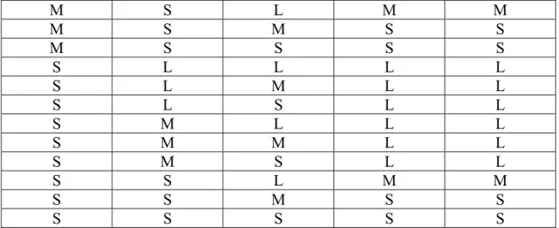
Table 9 The fuzzy rules of making a turn motion. Radius of Curve Velocity Length of Curve Variation

Percentage of Y Moving Rate of Y L L L L S L L M M S L L S S S L M L M M L M M S S L M S S S L S L S S L S M S S L S S S S M L L L L M L M M M M L S M S M M L M M M M M S S M M S S S Length of the slope Length of the slope Acceleration Acceleration Acceleration Length of the slope

M S L M M M S M S S M S S S S S L L L L S L M L L S L S L L S M L L L S M M L L S M S L L S S L M M S S M S S S S S S S

Table 10 The moving rate of Z fuzzy rules of downward slope.

Short Normal Long

Slow S S S

Normal L M S

Fast L M S According to the film offered by Occam Corp., we utilized the fuzzy rules to generate the platform position. Fig 13 is the surge variation of an upward slope motion, in which the solid line is the trajectory offered by Occam Corp. and the dash line is the trajectory generated by the fuzzy rule. Fig 14 is the sway variation of an turn right motion, in which the solid line is the trajectory offered by Occam Corp. and the dash line is the trajectory generated by the fuzzy rule.

Fig 13 The Surge(Y) variation.

Acceleration

Length of the slope

Fig 14 The Sway(Z) variation. 四、函數型類神經網路 (FFANN)

可是這樣的資料庫再使用上可能會很難，因為generalization 的能力是相當缺乏的。而 且此資料庫的型態是以函數為本質而不是點。在我們的研究中我們將研究利用 Function Artificial Neural Network(FANN) [23-26]來做 Motion cue 資料的建立。而在第一年的研究 中，由於其運動體就是操作者，所以其所需要的動作平台的模擬反應較小，而且是可預測 的。因此在研究上我們將考慮在我們先前研究中運動轉換資料庫的設計上，運動轉換資料 庫主要的概念是針對已知的運動行程(如動態電影院)，直接設計平台動作的方式，由於此部 分有些專家的經驗，因此針對如是的資料庫，我們可以累積經驗使之成為與被模擬機構及 平台機構無關的運動轉換法則，而為了能達到知識粹取的過程，利用類神經方式的建模是 值得探討的，除了其能利用recognition without definition 的特質質，其將知識參數化，也可 提供未來進一步學習修正的依據。

而在motion cue 的記錄方面，我們考慮使用函數型類神經網路來記錄 motion cue。在 傳統的類神經網路，通常以點對點的方式在時域當中進行系統的建構。而所建構的網路以 適應性網路進行網路鍵結值的學習。近來，一種函數型類神經網路架構已發表出來，函數 型網路架構使用數學的方式進行函數對函數的輸出輸入對訓練網路之鍵結值。因為函數型 網路使用平行處理之數學計算，可以快速估計出約略所需的輸出鍵結值。由於它優異的函 數近似能力，使得我們可以將其運用在系統之頻域響應當中。

FANN 在 1997 年的時候由 Newcomb 及 de Figueiredo 所發表出來的一種類神經網路 架構、整個的神經網路架構如圖15。其突破傳統神經網路以點對點的輸出輸入對的方式訓 練神經網路，而改用function 取代原本以 point 為主要架構。輸入、輸出、鍵節值皆以 function 來表示。而FANN 在鍵結值修正學習的機制裡為順向傳遞。由圖可見_{u L1}

() ()

⋅ u_n⋅為functional input，若u

( )

t =

{

u₁

( )

⋅_Lu_n

( )

⋅

}

，則n為它的取樣個數。輸入層與第一層隱藏層所連結的鍵結 值為pattern 的取樣值，進入第一層隱藏層之後，經過 Volterra series 的 model 所產生的值與 鍵結函數c₁

( )

t _Lc_n

( )

t 做乘加，所得出結果y₁

( )

t _Ly_n

( )

t 。其他的應用，還有參考資料[16]－ 含未知非線性系統之類神經網路控制，所發展新架構的FCPBUM，在傳統點對點的類神經 網路，為了達到良好的函數近似結果及快速收斂的目的，引用我們所發展的 CPBUM（以 契比雪夫多項式為基底的統一模型的類神經網路），在函數的學習上運用FANN，在學習架 構上使用 CPBUM，而達到更多的優點，包含最佳化的近似，及良好的內差能力之外，根 據相似度及靈敏度加入了知識拓展的優點。得以克服目前點對點神經網路在未知線性系統 軌跡追蹤學習的缺點。另外在[17]中，作者所提出的 D-FANN 架構。在文中發表一新式函 數型類神經架構，唯一非線性適應性時間序列預知器，以 discrete cosine transform basis function 為基底而產生的 filter bank 來做鍵結值，主要用來 model 一些非線性的動態訊號， 例如：人類的與音訊號。

圖15：MIMO FANN 基本架構 而在我們的未來工作之中，可望結而各種演算法，解決如輸入必須為能量有限的輸入 （即為非週期且遞減的輸入曲線）的缺點，例如sin 跟 cos 訊號的學習。藉由前置的離散訊 號處理以頻率域替代傳統的時間域學習，並期望在噪音的環境之下由在頻率域作業的優 點，而產生抑噪的功能；第二步，並將頻率分解，由FANN 的近似能力來學習，進而追蹤 期望訊號；第三步輸出並轉換為時間域。這個架構可結合訊號處理的優點（高速、抑噪）， 而達到我們想要的結果。目前FANN 正處於萌芽時期，其中尚有以上一些缺點必須解決， 對於週期性的輸入便無法辨識，還有當期望輸出上下限落差大，FANN 也無法學習，及鍵 結值的學習速度也在改進的範圍之中。希望藉由我們提出的架構來改善以上所提之缺點， 並提升神經網路的效能。FANN 以函數為輸出及輸入的類神經網路。而為了能進一步粹取 出轉換法則，我們也將使用Function Fuzzy Network(FFN)的方式來設計。FNN 的架構及其 學習效果等，都是本研究所要探討的。

FANN is a powerful and fast approach of modeling complex systems. All structure is developed by the mathematical theorem, named the Volterra series. The Volterra approach has been used for modeling nonlinear systems, when prior information is available about the internal characteristics of such systems or when the complexity of the system prevents the postulation of explicit parametric models.The identification problem of a single-input single-output (SISO) nonlinear dynamical system is considered in [26], under the assumption that the input-output relationship can be described by a Volterra series

( )

t =V

( )( )

u t =V

( )

u

( )

⋅ y _t

(

) ( )

( )

k k I t k k I t k dt dt t u t u t t t h k k ⋅⋅ ⋅ ⋅⋅ ⋅ ⋅ ⋅⋅ ⋅ ⋅⋅ ⋅ =

∑

∫

∫

∈ ∈ ∞ =0 1 1 1 , , ; ! 1 1 (3-1)

where the input u belongs to real L2

( )

I _{. I is an interval of the real line, and, for some}

nonnegative integer n, the output y is a member of the Sobolev space H_n2

( )

I _{of real-valued}

functions y on I such that _y( )i _=di_y/dti_{is absolutely continuous on I, i =0,1, ,n−1}

( ) _L

_{( )}

_I

y n _∈ 2 _{. On physical grounds, these conditions state that u and y and sufficiently many, n, of}

the output derivatives have finite energy by taking all such functions to be square integral over I.

It is proven in [26] that when a set of test pairs

{

(

u_j L2

( )

I ,y_j H_n2

( )

I

)

: j 1, ,N

}

L = ∈

∈ is

available, where , 1, , ,u j_{j = L} N are distinct elements of L2

( )

I _{, then the optimal estimate}

( )

u Vˆ_t of V_t

( )

u is

( )

_∑

( )

( ) ( )

=       _{⋅ ⋅} ⋅ = N j j j t u u r t c u V 1 , 1 exp ˆ _(3-2) where

( ) ( )

_{( )}

∫

( ) ( )

∈ = ⋅ ⋅ I t I L u t vt dt v u , 2 and w_j H_n

( )

I 2 ∈ are obtained by (3-2)

( )

( )

( )

( )

         ⋅ =           − t y t y G t w t w N N M M 1 1 1 , (3-3)

( ) ( )

_{( )} N j i I L j i u u r G , , 1 , 2 , 1 exp L =             _{⋅ ⋅} = (3-4) The set of test pairs,

{

(

u_j L2

( )

I ,y_j H_n2

( )

I

)

: j 1, ,N

}

L = ∈

∈ that describe (12), serve like exemplars of artificial neural networks. This leads to the development of FANN [9][10], which implements as a feed-forward neural network with functional weights c_j

( )

⋅ . In this respect, exemplars of functions while conventional neural networks are trained with exemplars of point values.

The block structure of FANN may be realized as a two hidden layer network [25], where the synaptic weight associated with the connection from u

( )

k to the _{j neuron of the first layer} th

represents the value uj

( )

k _{of the j exemplar input. The output of each neuron in the first} th

layer being exponential over the sum of weight input products. The second hidden layer consists of a single linear neuron, with synaptic weights w_j

( )

t and output equal to y

( )

t .

The FANN under consideration, implements an operator that is an optimal L₂ interpolation map of a function u

( )

⋅ into another function y

( )

⋅ over a time interval I, according to the

formula:

( )

( )

( )

( )

( ) ( )

      _{⋅ ∆} ⋅ = ⋅ =

∑

∑

= = Ns k j N j j u k u k t r t w t V t y T 1 1 1 exp (3-5)

for input over discrete time of N samples. In general, u

( )

t and y

( )

t are vectors of real values at time t; i.e., u

( )

⋅ consists of n elements being functions of t, and y

( )

⋅ consists of m elements

being functions of t, resulting in a multiple-input multi-output functional artificial neural network.

The patterns

{

{

uj

( )

t _,t_{∈ 1}I

}

_{, ≤} j_≤ N

}

_{are exemplar inputs for training the network. In the}

implementation of a FANN, the exemplar training inputs _uj

( )

⋅ _{are represented by N samples in} the time interval I, and treated as weight vectors for the first of the two layers of the FANN.

During training, w_j

( )

t is calculated for discrete time instances, or else it is modeled as a continuous vector function. Given an unknown pattern

{

u

( )

t ,t∈I

}

, FANN evaluates the similarity of this pattern to each of the exemplars

{

{

uj

( )

t _,t_{∈ 1}I

}

_{, ≤} j_≤ N

}

_{, and estimates y}

( )

_⋅

through weighted average of high selectivity over the corresponding exemplar actions _yj

( )

⋅ _,

where the degree of selectivity may be adjusted through r. Thus, if u

( )

⋅ is very similar to _uk

( )

⋅

and quite dissimilar from all other exemplars _ui

( )

⋅ _{, then y}

( )

_{⋅ is approximated by y}k

( )

_{⋅ .}

FANN was further generalized to multiple-input multi-output (MIMO) cases, by replacing

( )

I L2 _{with L}

( )

_I n 2 _and

( )

[

( )

( )

]

T n u u

( )

[

( )

( )

]

T m

y y

y⋅ = ₁ ⋅,_L, ⋅ is a vector of m functions. Also, the index j is placed as a superscript in

the MIMO case (it was a subscript in the SISO case) in order to avoid confusion with indexing the elements of the vector. Then

( )

( )

( )

_∑

( )

_∫

( ) ( )

= ∈      ⋅ ⋅ ⋅ = ⋅ = N j I j j t u u d r t w u V t y T 1 1 exp τ τ τ τ , (3-6) where r is a positive real constant,

{

( )

1

( )

, ,

( )

:

}

, 1

T

j j j

n

u t =_u t _L u t _ t∈I ≤ ≤j N are N prototype output patterns,

{

( )

1

( )

, ,

( )

:

}

, 1

T j j j n y t =_y t _L y t _ t∈I ≤ ≤j N with

( )

( )

( )

( )

( )

( )

1 1 1 T T T T T T i j N N w t y t G w t y t w t y t −              _{= •}                      M M M M (3-7) and G=

[ ]

G_ij where

( ) ( )

_      ⋅ ⋅ =

∫

∈I j i ij u u d r G T τ τ τ τ 1 exp . (3-8)

The set of test vector I/O function pairs,

{

(

uj_,yj

)

_: j _{1, ,}N

}

L

= are the exemplars for training the FANN, i.e., calculating the set of vector functional weight

{

wj

( )

t _:t_{∈ 1}I

}

_{, ≤} j_≤N _.

If an unknown input pattern

{

u

( )

t :t∈I

}

is presented, the FANN evaluates the similarity of this pattern to each of the exemplars

{

uj

( )

t _:t_∈I

}

_{,1≤ j≤ N, and the estimates y(t) through}

weighted averaging of high selectivity over the corresponding exemplar outputs yj(t)_{, where} the degree of selectivity may be adjusted through γ . From (3-7) and (3-8), notice that wj

( )

t _is

inversely proportional to the exponential of the inner product of uj

( )

t _{with each of the}

prototype input patterns, and it is proportional to yj(t)_{. Notice (3-6), w}j

( )

_{t is multiplied by the}

exponential of the inner product of uj

( )

t _{with the input pattern u}

( )

_{t . In this configuration, the}

exponential terms define normalized weights that emphasize similarity in the averaging. Low selectivity results in smooth averaging over the exemplar outputs, while high selectivity results in a crisper approximation where the output that corresponds to the exemplar input that best matches

( )

⋅

u is emphasized in the averaging. Thus, if u

( )

⋅ is very similar to uk

( )

t _{and quite dissimilar}

from all other exemplars ul

( )

t _{, then y(t) is approximated by y}k

( )

_{t . If the similarity of u}

( )

_⋅

to more than one exemplar input is high, then y(t) is approximated as an average over their corresponding exemplar outputs weighted by a measure of the corresponding similarities.

The following is listed the algorithm of the FANN,

Training Phase

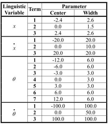
Step 1. Set the numbers of input layer neurons, second layer neurons, and output layer neurons.

The weights between the first layer and second layer are defined in (3-8). From (3-8), the parameter γ is needed.

Step 2. Forward the input x

[ ] [ ]

n =un into the first layer.

Step 3. By (3-8), the matrix of second layer neurons, G , is calculated. _ij

Step 4. By (3-6), compute the output sequence of output layer neurons,Y . From (3-7), the

weights between second layer and output layer are calculated. These are the output weights we want.

There is something to be noticed. In the training phase, the algorithm of FANN does not have the learning procedure. That may infect the accuracy of the output, y

( )

t .

Testing Phase

Step 1. Forward the input testing exemplars into the first layer.

Step 2.The weights between the first layer and second layer as step 1 in training phase is used

to compute G using (3-8). _ij

Step 3.The weights between the first hidden layer and the output layer as step 4 in training

phase is used to compute testing output sequence, y

[ ]

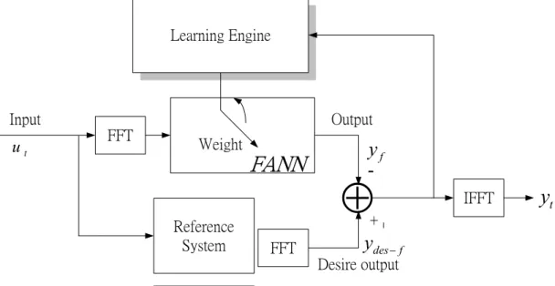
n .

The structure of the FANN in the frequency domain is now proposed. A main difficulty for neural networks working in the frequency domain is that they need complex-valued weights for the networks. Because of complex-valued weights, there are four algorithms are discussed. In order to perform learning for this situation, the structure of FANN must be modified. The modification is to provide mechanism for transferring training data in the time domain into the frequency domain and to improve the performance, as we require. In the first, a FANN-based neural network is constructed. To consider signals in the frequency domain, the fast Fourier transform and inverse fast Fourier transform are necessities. In this stage, some details about sample points and aliases are important to reconstruct signals in the time domain.

It is well known that when the analysis or design of a system is conducted in the frequency domain, the result should be more robust to noisy and/or outliers compared to that in the time domain. For analysis in the frequency domain, sometimes, a discrete low pass filter is required. In our study, the Kaiser window [32] is employed to design such a low pass filter. The Kaiser window is defined as

[ ]

[

(

[

(

_{( )}

)

]

)

]

, , 0 , 0 1 0 2 1 2 0 otherwise M n I n I n w ≤ ≤      _{− −} β α α β

where α =M 2, and I₀

( )

⋅ represents the zero-order modified Bessel function of the first kind. The Kaiser has two parameters: the length

(

M +1

)

and a shape parameter β. Let ω_s be the stop-band cutoff frequency and ω_p be the pass-band cutoff frequency, the width of the transition region is defined as ∆ω =ω_s −ω_p. Define A=−20log₁₀δ . The value of β is given by

(

)

(

)

(

)

, 21 50 21 , 50 , 0 . 0 , , 21 07886 . 0 21 5842 . 0 , 7 . 8 1102 . 0 4 . 0 < ≤ ≤ >      − + − − = A A A A A A β .

Then M must satisfy

ω ∆ − = 285 . 2 8 A M .

The structure of our functional network networks is shown in Fig. 16. In the FANN, the approximated function is obtained through (3-2~3-4). The functions give the FANN a roughly range of global minima. But the network cannot find the optimal output near the desire output. For BP or FP (forward propagation) types of learning algorithms, their learning is usually slow and has several local minima. In [28], the approach of mixing the BP learning algorithm and the original algorithm used for FANN was proposed and the learning of that approach is fast and powerful in finding global minima.

There are four algorithms used in our implementation of the FANN in the frequency domain. First, the original algorithm of the FANN is still used. That is the FANN in the frequency domain without learning. It is the traditional FANN.

Reference System Learning Engine Input Output Desire output

⊕

-

₊ Weight FFT

FANN

FFT IFFT t u f des

y

₋ f

y

t

y

Fig. 16 The modified structure of FANN

Algorithm 1.

Step 1. Transform all signals into the frequency domain. All signals become complex data. Step 2. Set the numbers of neurons in the input layer, in the second layer neurons, and in the

output layer neurons, respectively.

Step 3. Set weights between input layer and hidden layer as exemplars. Step 4. Compute the values G of neurons in the second layer by using (3-4). _ij

Step 5. Compute the output values Y of neurons in the output layer by using (3-5). _i

Step 6. Compute the weights between the second layer and the output layer by using (3-3). Step 7. Input the testing signals and compute the output signals by the weights.

Step 8. Transform the output signals into the time domain.

Because complex-valued parameters are used for representing signals in the frequency domain, CNET (Complex-valued weight Neural Network) is proposed to model systems in [28-31]. The error signals are defined as εi

[ ]

i = ydes−f,i

[ ]

n −yf,i

[ ]

n , i,n=1,2,L,N [30]. Then,

the cost function is usually defined as the sum of squared errors and is

[ ]

_∑

[ ] [ ]

= ⋅ = N i i i n n n E 1 ε ε , (3-9)

where ε_i

[ ]

n is conjugate of ε_i

[ ]

n . The BP algorithm minimizes the cost function (3-9) by recursively altering the weights based on the gradient search technique. The partial derivative of

E with respect to the real and imaginary part of the weights must be derived separately. Let

[ ]

n wr

[ ]

n iwi[n]

w_ij = _ij + . (3-10) Consider the adaptation rule of the output layer as

[

]

[ ]

_{[ ]}

n wr n E n wr n wr ij ij ij _∂ ∂ − = + µ 2 1 ] [ 1 (3-11)

[

]

[ ]

[ ]

n wi n E n wi n wi ij ij ij _∂ ∂ − = + µ 2 1 ] [ 1 . (3-12)

Combining (3-11) and (3-12), we have

[

]

[

]

[ ]

[ ]

_       ∂ ∂ + ∂ ∂ − + = + + + ] [ ] [ ] [ ] [ 2 1 1 1 n wi n E i n wr n E n iwi n wr n iwi n wr ij ij ij ij µ (3-13) or

[

]

[ ]

_       ∂ ∂ + ∂ ∂ − = + ] [ ] [ ] [ ] [ 2 1 1 n wi n E i n wr n E n w n w ij ij ij µ (3-14) and wr y y z z E wr y y z z E wr E f f f f ∂ ∂ ⋅ ∂ ∂ ⋅ ∂ ∂ + ∂ ∂ ⋅ ∂ ∂ ⋅ ∂ ∂ = ∂ ∂ , (3-15)

where z = f

( )

y_f ,y_f =

∑

wu_f +θ . They are commonly used in neural networks. f is the sigmoidal function and is defined as

( )

_y

e y f ₋ + = 1 1 . Then,

(

ydes f yf

) ( ) (

f yf uf ydes f yf

) ( )

f yf uf wr E _{=− − ′ − − ′} ∂ ∂ − − . (3-16) Similarly, i

(

y_{des f} y_f

) ( )

f y_f u_f i

(

y_{des f} y_f

) ( )

f y_f u_f wi E _′ − + ′ − − = ∂ ∂ − − . (3-17)

Combining (3-16) and (3-17), we have

(

y_{des f} y_f

) ( )

f y_f u_f wi E i wr E _′ − − = ∂ ∂ + ∂ ∂ − 2 . (3-18) Substituting (3-18) into (3-13) wi_ij

[

n+1

]

=wi_ij[n]+µ

(

y_des−f −y_f

) ( )

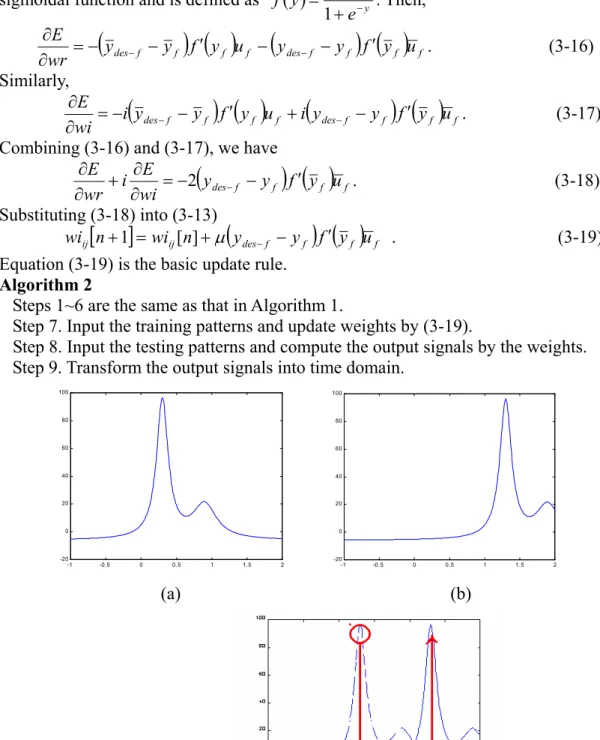
f′ y_f u_f . (3-19) Equation (3-19) is the basic update rule.

Algorithm 2

Steps 1~6 are the same as that in Algorithm 1.

Step 7. Input the training patterns and update weights by (3-19).

Step 8. Input the testing patterns and compute the output signals by the weights. Step 9. Transform the output signals into time domain.

-1 -0.5 0 0.5 1 1.5 2 -20 0 20 40 60 80 100 -1 -0.5 0 0.5 1 1.5 2 -20 0 20 40 60 80 100 (a) (b) (c)

Fig. 17 (a) The output before learning (b) The desire output (c) The algorithm must to depress the signal we do not want and grows the wanted signal up.

There exist problems in the above algorithm. The learning procedure updates the real and imaginary parts of the weights. Algorithm 2 uses only one learning rate to tune the weights and the range of the real part value is different from that of the imaginary part value. That means if the range of the real part value is [–50, 50], the range of imaginary part may be [–0.5, 0.5]. By the algorithm in traditional FANN, the input signals and output signals of FANN do not have to normalization to [–1, 1]. As a consequence, the updated weights are not optimal. The other problem is the disturbance. The trace after learning is like the desired trace plus a sinusoid with a fixed frequency. The phenomenon is shown in Fig. 17. The output contains a small impulse in the amplitude of the Bode plot. It is obvious that the obtained amplitude is not what we want. After

the signal is reconstructed in the time domain, such an unwanted impulse in the frequency domain becomes a sinusoid in the time domain.

The complex numbers can be expressed as the following form: (a) (real part) + (imaginary part) j (3-20) (b) (amplitude) × _ej( phase) _(3-21)

In the next discussion, we separate the complex numbers into two neural networks. In (3-20), the FANN (a) is to model the real part of the complex-valued weights and the FANN (b) is to model the imaginary part. Similarly, in (3-21), the FANN (a) is the neural network to define the amplitude of the complex-valued weights and the FANN (b) is to define the phase of the complex-valued weights. Note that the learning rate in FANN (a) is different from that in FANN (b).

Algorithm 3 with ((real part) + (imaginary part) j) method Step 1~6 are the same as those in Algorithm 1.

Step 7. In the FANN (a), input the training patterns (the real part of all signals) and update weights by (3-19) in the FANN (a).

Step 8. Input the testing patterns (the real part of all signals) and compute the output signals (the real part of all signals) by the weights.

Step 9. Do Step 1~8 for the FANN (b). The output signals (the imaginary part of all signals) are calculated.

Step 10. Combine the real part and the imaginary part into complex numbers. Step 11. Reconstruct the signal in the time domain.

Algorithm 4 with (amplitude) × _ej( phase) _method

Step 1~6 are same as the Algorithm 1.

Step 7. In the FANN (a), input the training patterns (the amplitude of all signals) and update weights by (3-19) in the FANN (a).

Step 8. Input the testing patterns (the amplitude of all signals) and compute the output signals (the amplitude of all signals) by the weights.

Step 9. Do Step 1~8 for the FANN (b). The output signals (the phase of all signals) are calculated.

Step 10. Combine the amplitude and the phase into complex numbers. Step 11. Reconstruct the signals in the time domain.

In Algorithm 4, updating amplitude and phase is very sensitive in time domain. Algorithm 3 overcomes the disadvantages mentioned for Algorithm 2 and Algorithm 1. The network learns the system quickly and robust. The tracking performance is better than that of the FANN in the time domain. To reserve the idea of the FANN, all the structures and algorithms in our implementation follow the formula in equation (3-8). In other words, all weights between the hidden layer and input layer are not updated.

Fig. 18 Example and the parameters we define

The case of a car and a driver-system, which was also used in [8], is used as an example in our implementation. In this example, the output is expressed by its moving direction. The goal of

the driver-system is to keep the car on the road. As shown in Fig. 18, this car is assumed to move on a path resides on the X_W −Y_W plane of the world coordinate system (WCS). The desired path is represented as a function of traveling time t. Let a point on the path then can be expressed as a parametric pair, like

(

x_w

( ) ( )

t ,y_w t

)

and φ be the angle of the slope of this path at a point

( )

t through t and is obtained as

( )

t ₌tan−1

(

dy_w

( )

t /dx_w

( )

t

)

φ (3-22)

Then, the sequence

{ }

φ

( )

t represents the shape of the path. Define θ as the angle between

( )

t the central axis across the car and the X axis of the WCS. Then _W θ denotes the direction of

( )

t the car. The driver’s goal, which is to keep the car remaining on the road, then can be expressed through the relation θ

( ) ( )

t =φ t . The action of the driver-system at time t is the amount of angle

( )

t

w by which the system must turn the wheels with respect to the central axis across the car to keep the relation θ

( ) ( )

t =φ t satisfied for each t.

The road is modeled as a composition of segments, where each segment may be a path as a straight line or a concave path forming a turn. Assuming a minimum resolution time ∆t by which the driver-system scans the road ahead at a speed U , the road segments are sampled at _s

intervals ∆S =U_s⋅∆t. Each road segment then is modeled as a discrete-time sequence of angles of slopes

{

_φ

( )

_i :_t=_i×∆_t,_i∈_Z+ ∪

{ }

0

}

_{. The driver-system has a perspective view of the road} ahead, instead of its actual floor plan. Thus, it views a transformed image of the road ahead. Consequently it perceives a discrete-time sequence of angles of slopes

( )

{ }

{

_{σ i} :_t =_i×∆_t,_i∈_Z+ ∪ 0

}

_{on the transformed image. This sequence is used by the}

driver-system in order to plan its actions; i.e., to generate a sequence

( )

{ }

{

_i :_t =_i×∆_t,_i∈_Z+ ∪ 0

}

p

ω before the car enters the viewed road segment. When the car enters the road segment, t =i×∆t will be tan

( )

θ

( )

i , where θ

( ) ( ) ( )

i =θ i−1 +ω i−1 , or equivalently, θ

( ) ( )

i =θ 0 +

∑

i_k−₌1₀ω

( )

k , and ω

( )

i is determined by ω

( )

i =ω_p

( )

i +∆ω_p

( )

i . Here

p

ω is the input u and _p ∆ω_p is the correction through feedback.

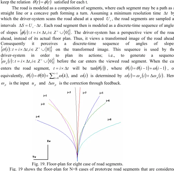
Fig. 19. Floor-plan for eight case of road segments.

Fig. 19 shows the floor-plan for N=8 cases of prototype road segments that are considered for training the FANN. In this example, each of those paths were generated by a third degree polynomial, 0 1 2 2 3 3 x a x a x a a y_w = ⋅ _w + ⋅ _w + ⋅ _w + (3-23)

where the variables x and _w y refer to the coordinates of each point along the path. This is the _w

least degree of polynomial that satisfies continuity in position and slope at both ends of each segment and allows their smooth concatenation in modeling general shapes of paths. Since it is desired that

{ }

θ

( )

t =

{ }

φ

( )

t , we need to have the sequence

{ }

φ

( )

t for each of the prototype

patterns to train the FANN. Since the prototype path segments are generated by a third degree polynomial, the angle of the tangent at each point along the path is given as

( )

(

( )

2

( )

1

)

2 3 1 1 _{tan 3 2} tan a x t a x t a dx dy t _{w w} w w _{= ⋅ ⋅ + ⋅ ⋅ +}       = − − φ . (3-24)

The origin of each path is at the point

(

x_w

( )

0,y_w

( )

( )

0

) ( )

= 0,0 and then a₀ =0. The slope of the tangent at the origin of each path is zero coinciding with the direction of the car as it enters the path segment, and also a₁ =0. This assumption is natural in this example, because the driver-system may consider a single road segment head of it each time when the car is located at the origin of that segment. Besides, at that time, the moving direction of the car should coincide with the slope at the origin of the segment for a smooth ride. Then, it is also natural to perceive that segment as if it were described with reference to a world coordinate system whose origin coincides with the driver’s position and the X axis coincides with the moving direction of the _w

car. Then, a straight segment becomes trivial since a₃ =a₂ =a₁ =a₀ =0, and thus φ

( )

t =0 at each point along the segment. For this reason, we did not include a straight segment among the eight prototypes in this example, although we could have.

The X axis is calculated as _W

x_w

( )

i =x_w

( )

i−1 +Ur_S ⋅∆t⋅cos

( )

φ

( )

i , (3-25)

( )

(

2

( )

₂

( )

₁

)

3 1 _{3 1 2 1} tan a x i a x i a i ≈ − ⋅ ⋅ _w − + ⋅ ⋅ _w − + φ , (3-26) and thus,

( )

( )

(

(

( )

2

( )

1

)

)

2 3 1 _{3 1 2 1} tan cos 1 U t a x i a x i a i x i x_w = _w − + r_S ⋅∆ ⋅ − ⋅ ⋅ _w − + ⋅ ⋅ _w − + _{, (3-27)} where ω is calculated as

( )

i ω

( )

i =∆φ

( ) ( ) ( )

i =φ i+1 −φ i (3-28)

Next, the restoration map of the perceived image is calculated. Let

[

C_X,C_Y,C_Z

]

be the world coordinates of the driver’s camera, N =

[

N_X,N_Y,N_Z

]

be the viewing direction of the camera, Vr be a view-up vector that specifies the orientation of the camera, and d be the distance of lens from its screen. Choosing Lr =Vr×Nr results in a right-hand viewing coordinate system (Lr,Vr,Nr ) centered at the lens of the camera. Then, a viewing transformation is used in order to map world coordinates

[

x_w,y_w,z_w

]

to viewing coordinates

[

x_v,y_v,z_v

]

, and subsequently a perspective transformation maps the viewing coordinates to screen coordinates

[

x_s,y_s,d

]

. The angle of slope σ that is perceived at each point on the transformed image on the screen of the

( )

t camera is a mapping of φ , and is calculated as

( )

t

( )

t _=tan−1

(

dy_s

( )

t dx_s

( )

t

)

σ . (3-29) Differentiation by parts, s w w s s s dx dy dx dx dx dy = ⋅ (3-30) followed by long calculations, (3-29) becomes