使用平行化直接模擬蒙地卡羅法初步模擬在稀薄流體範圍時瞬間啟動的空穴超音速流場

(1)

國立交通大學

機

械

工

程

學

系

碩士論文

使用平行化直接模擬蒙地卡羅法初步模擬在稀薄流體

範圍時瞬間啟動的空穴超音速流場

Preliminary Simulation of Instantaneously Started

Supersonic Driven Cavity Flows in the Rarefied Gas

Regimes Using the Parallel Direct Simulation Monte Carlo

Method

研究生：洪維呈

指導教授：吳宗信博士

(2)

使用平行化直接模擬蒙地卡羅法初步模擬在稀薄流體範圍時瞬間啟動的空

穴超音速流場

Preliminary Simulation of Instantaneously Started Supersonic Driven Cavity

Flows in the Rarefied Gas Regime Using the Parallel Direct Simulation Monte

Carlo Method

研究生：洪維呈 Student: Wei-Cheng Hung

指導教授：吳宗信博士 Advisor: Dr. Jong-Shinn Wu

國立交通大學

機械工程學系

碩士論文

A Thesis

Submitted to Institute of Mechanical Engineering

College of Engineering

National Chiao Tung University

in partial Fulfillment of the Requirements

for the Degree of

Master of Science

in

Mechanical Engineering

July 2007

Hsinchu, Taiwan

中華民國九十六年七月

(3)

致謝

在交大兩年的求知路程，特別感謝指導教授吳宗信老師的照顧，讓我在學習過程及生活方面都得到不少獲益。在研究及做學問方面，與老師的知識交流實令我感到獲益匪淺，讓我能順利的踏入研究的領域並且不斷地成長。還有老師愛台灣精神及推廣本土文化不遺餘力也在我心中根深蒂固。同時也感謝口試委員黃俊誠老師、郭添全博士、陳明志老師在口試時提供的寶貴意見，使得本論文更加充實完備。另外特別感謝曾坤璋學長長期發展關於此篇論文中所用到的程式之辛勞，且在最後兩個月不吝於付出時間與心力來教導我於研究中所遭遇的問題，以及粲哥、凱文兄在研究上啟發教導及生活上的鼓勵幫助，在此一併致謝。要感謝的人太多，邵雲龍、許國賢、陳育進、梁偉豪、陳百彥等已畢業的學長，還有 APPL 實驗室的成員，李允民、周欣芸、李富利、洪捷粲、許哲維、鄭凱文、胡孟樺、邱沅明、江明鴻學長姊指導受益良多，盧勁全、謝昇汎、林宗漢、陳又寧、王柏勝同學，與你們努力奮鬥相處的時光將是我最美好的回憶，正勤、士傑、志良、玟琪、丞志、政霖、育宗等學弟妹們協助，以及來自紐西蘭的訪問學者 Hadley M. Cave (瓦片)，使我這兩年過得相當充實且溫馨，並能順利完成學業。此外最後特別感謝我的大學指導教授牛仰堯導師，感謝他對我的期許鼓勵及愛護，我會更加努力朝向目標邁進，以及陪伴我的家人，辛苦了。在這離別季節，大家各自奔向前程，希望大家追求自己的夢想前進，擁有光明未來和生活。洪維呈謹誌九六年七月于風城

(4)

使用平行化直接模擬蒙地卡羅法初步模擬在稀薄流體範圍時瞬間

啟動的空穴超音速流場

學生: 洪維呈指導教授: 吳宗信

國立交通大學機械工程學系

摘要

空穴流場是ㄧ個很基本的流體力學問題，在過去也有很多人做過相關的研究。但是大多數人都是討論連續及不可壓縮流流場，較少數人針對連續流到稀薄流體區的流場作研究。因此我們對此做ㄧ有系列的探討。本文的目的為使用直接模擬蒙地卡羅法及非結構性網格來模擬從自由分子流到接近連體流體範圍瞬間啟動的空穴超音速流場。傳統上在模擬稀薄區中，非穩態流場較少人研究，也較困難。我們先運用非穩態的時間平均取樣方法來模擬，但發現有大量 scatter 現象。因而我們運用 DSMC-DREAM (Rapid Ensembled Average Method) [Cave et al., 2007] 可運用在減少統計時產生的 scatter 時間平均的 DSMC 資料，也為了確保能在較鄰近的分子發生碰撞，運用 transient sub-cells 在非結構性網格功能，使得同時降低計算負荷及記憶體使用量。

(5)

穩態驅動空穴流場條件包含上板驅動速度馬赫數 4 和 Knudsen 數(與平均自由路徑和空穴大小有關)由 10 到 0.0033。結果顯示其速度滑動現象會在 Knudsen 數的影響中表現的很明顯。在 Knudsen 數 0.1， 0.01 和 0.0033 的渦流幾何中心隨時間改變後會朝向幾何中心; 但 Knudsen 數 10 和 1 則往上板移動。而由於本文為初步模擬在非穩態的流場現象，所以先模擬在高馬赫 4 的流體。然而模擬此空穴超音速流場仍然有些統計樣本造成的 scatter 誤差現象。所以在未來會使用 temporal variable time step 來減少計算時間，及同時增加 DSMC-DREAM (Rapid Ensembled Average Method) [Cave et al., 2007] 循環次數，來大大減低此 scatter 誤差現象。

(6)

Preliminary Simulation of Instantaneously Started Supersonic Driven

Cavity Flows in the Rarefied Gas Regime Using the Parallel Direct

Simulation Monte Carlo Method

Student: Wei-Cheng Hung Advisor: Dr. Jong-Shinn Wu

Department of Mechanical Engineering

National Chiao-Tung University

Abstract

The driven cavity flow is one of the fundamental problems in the fluid dynamics. The

kind of topic establishes the foundation in computational fluid dynamics and its simple

geometry. However they have been completely studied in the literature, most of researches

focused on incompressible or continuum compressible regime. Very few researches have been

done in the rarefied and near continuum regimes. It may serve as the benchmarking problem

in these regimes. Therefore, this thesis reports the simulation of instantaneously started

supersonic driven cavity flows from the free-molecular to near-continuum regime using the

parallel direct Monte Carlo method using unstructured grids. A special technique called

DSMC-DREAM (Rapid Ensembled Average Method) was applied to reduce the statistical

scatter of time-averaging DSMC data. To ensure nearest-neighbor collision, transient

sub-cells are also implemented on an unstructured grid. Implementation was verified by

(7)

an acceptable runtime for unsteady flow simulation using DSMC technique. Simulation

conditions for the unsteady top driven cavity flows include Ma=4 of the speed of top driven

plate and Kn=10-0.0033 based on the mean free path of wall temperature and size of the

cavity. Results show that the velocity slips along the solid walls increase with increase

Knudsen number at the same Mach number (M=4). Center of the primary vortex during one

time moves towards the geometric center with Knudsen number is 0.1, 0.01 and 0.0033. Other

cases move toward the upper wall with Knudsen number is 10 and 1.Because the thesis is

preliminary study on unsteady flow, thus we focus on supersonic flow (M=4). There are

scatter on simulation supersonic cavity flow; hence it will use temporal variable time step to

induce computational cost and increase DSMC-DREAM (Rapid Ensembled Average Method)

run times. Further, the imperfection of results are on Knudsen number 10 (free molecular

flow), 1 and 0.1 because of the mean free path larger than characteristic length. Thus, particles

(8)

List of Tables

Table I Flow and simulation condition for 1-D Couette flow. ... 43

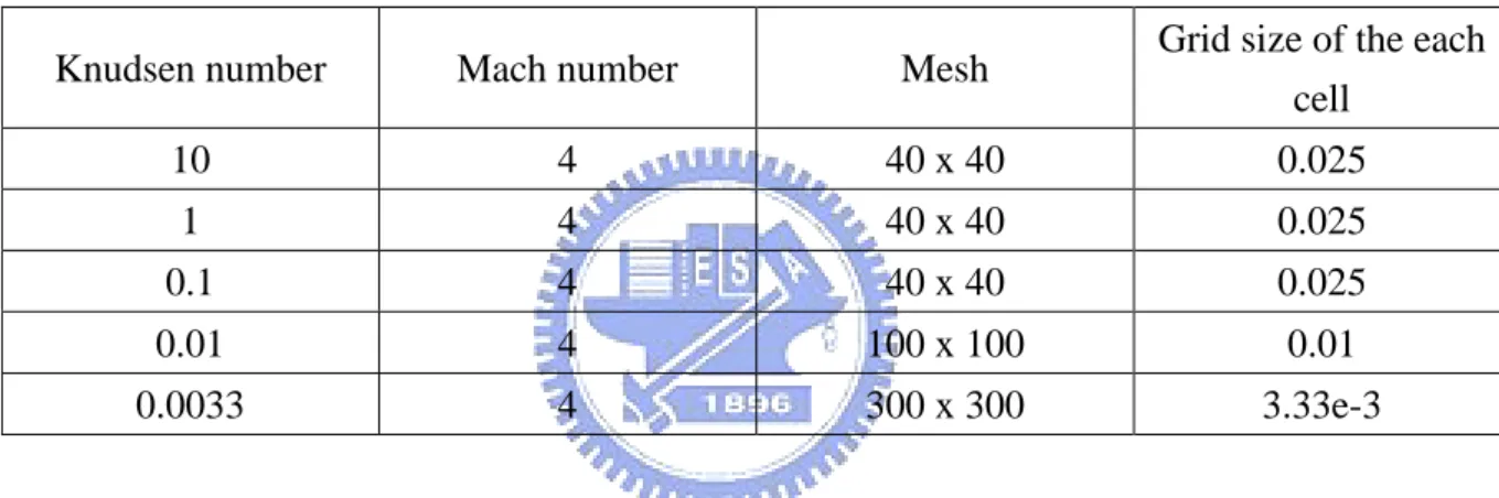
Table II The grid sizes of distinct driven cavity cases. ... 44

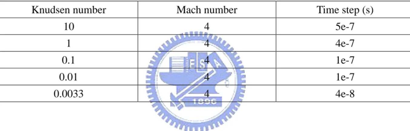
Table III The time steps of distinct driven cavity cases. ... 45

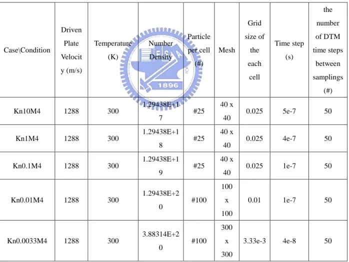
Table IV The initial conditions of distinct driven cavity cases. ... 46

Table V The other conditions of distinct driven cavity cases... 47

(11)

List of Figures

Fig. 2.1 Classifications of Gas Flows ... 49

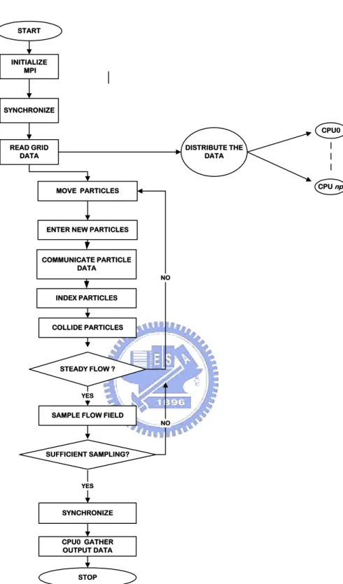
Fig. 2.2 Flow chart of the DSMC method ... 50

Fig. 2.3 Simplified flow chart of the parallel DSMC method for np processors. ... 51

Fig. 2.4 The additional schemes in the parallel DSMC code... 52

Fig. 2.5 Sampling method in DSMC include (a) steady sampling (b) unsteady ensemble sampling (c) unsteady time averaging. ... 53

Fig. 2.6 Simplified flow chart of the unsteady parallel DSMC method. ... 54

Fig. 2.7 Simplified flow chart of the DSMC Rapid Ensemble Averaging Method (DREAM) ... 55

Fig. 3.1 Computational domains for the developing Couette flow. ... 56

Fig. 3.2 The mesh (100x100) for M=0.3, Kn=0.02 Couette flow. ... 57

Fig. 3.3 Contours of velocity for M=0.3, Kn=0.02 Couette flow from unsteady DSMC technique at normalized time (a) t =1; (b) t=3; (c) t=7; (d) t=16; (e) t=32 ... 58

Fig. 3.4 Comparison of for M=0.3, Kn=0.02 Couette flow development by unsteady DSMC (symbols) with the exact Navier-Stokes solution (lines). ... 59

Fig. 3.5 Contours of velocity for for M=0.3, Kn=0.02 Couette flow from DREAM technique at normalized time (a) t =1; (b) t=3; (c) t=7; (d) t=16; (e) t=32 60

Fig. 3.6 Comparison of for M=0.3, Kn=0.02 Couette flow development by unsteady DSMC with the DREAM technique at normalized time (a) t=1; (b) t=3; (c) t=7; (d) t=16; (e) t=32 ... 61

Fig. 3.7 Comparison of for M=0.3, Kn=0.02 Couette flow development by unsteady DSMC with the DREAM technique (symbols) with the exact

Navier-Stokes solution (lines). ... 62

Fig. 3.8 The mesh for x y

 

 

 =0.25 for M=0.3, Kn=0.02 Couette flow. ... 63

Fig. 3.9 Contours of velocity for x y

 

 

 =0.25, for M=0.3, Kn=0.02 Couette flow. ... 64

Fig. 3.10 Contours of mcs/mfps for x y

 

 

 =0.25, for M=0.3, Kn=0.02 Couette flow. ... 65

Fig. 3.11 the mesh for x y

 

 

 =1 for M=0.3, Kn=0.02 Couette flow. ... 66

Fig. 3.12 Contours of mcs/mfps for x y

 

 

(12)

Fig. 3.14 Comparison of Couette flow development by x y      =0.25 with x y      =1. ... 69

Fig. 3.15 The 2D square (L/H=1) driven cavity flow with moving top plate. ... 70

Fig. 3.16 the mesh (40x40) for Kn=10, 1, 0.1 driven cavity flow. ... 71

Fig. 3.17 the mesh (100x100) for Kn=0.01 driven cavity flow. ... 72

Fig. 3.18 the mesh (300x300) for Kn=0.0033 driven cavity flow. ... 73

Fig. 3.19 Contours of u-velocity for M=4, Kn=10 at (a) t =50s; (b) t =125s; (c) t =225s; (d) t =325s; (e) t =425s; (f) t =600s; (g) t =1500s; (h) t =3000s ... 74

Fig. 3.20 Contours of u-velocity for M=4, Kn=1 at (a) t =40s; (b) t =100s; (c) t =180s; (d) t =320s; (e) t =480s; (f) t =700s; (g) t =1100s; (h) t =1800s ... 75

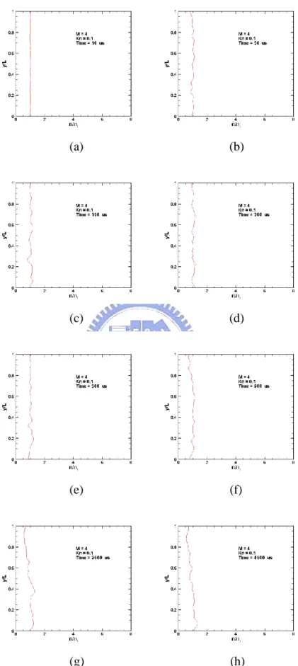
Fig. 3.21 Contours of u-velocity for M=4, Kn=0.1 at (a) t =10s; (b) t =50 s; (c) t =150s; (d) t =300s; (e) t =500s; (f) t =900s; (g) t =2500s; (h) t =4500s ... 76

Fig. 3.22 Contours of u-velocity for M=4, Kn=0.01 at (a) t =10s; (b) t =75s; (c) t =175s; (d) t =300s; (e) t =500s; (f) t =900s; (g) t =1750s; (h) t =3750s ... 77

Fig. 3.23 Contours of u-velocity for M=4, Kn=0.0033 at (a) t =10s; (b) t =40s; (c) t =120s; (d) t =400s; (e) t =800s; (f) t =1200s; (g) t =1800s; (h) t =2650s ... 78

Fig. 3.24 Contours of v-velocity for M=4, Kn=10 at (a) t =50s; (b) t =125s; (c) t =225s; (d) t =325s; (e) t =425s; (f) t =600s; (g) t =1500s; (h) t =3000s ... 79

Fig. 3.25 Contours of v-velocity for M=4, Kn=1 at (a) t =40s; (b) t =100s; (c) t =180s; (d) t =320s; (e) t =480s; (f) t =700s; (g) t =1100s; (h) t =1800s ... 80

Fig. 3.26 Contours of v-velocity for M=4, Kn=0.1 at (a) t =10s; (b) t =50 s; (c) t =150s; (d) t =300s; (e) t =500s; (f) t =900s; (g) t =2500s; (h) t =4500s ... 81

Fig. 3.27 Contours of v-velocity for M=4, Kn=0.01 at (a) t =10s; (b) t =75s; (c) t =175s; (d) t =300s; (e) t =500s; (f) t =900s; (g) t =1750s; (h) t =3750s ... 82

Fig. 3.28 Contours of v-velocity for M=4, Kn=0.0033 at (a) t =10s; (b) t =40s; (c) t =120s; (d) t =400s; (e) t =800s; (f) t =1200s; (g) t =1800s; (h) t =2650s ... 83

(13)

Fig. 3.29 Contours of Mach number for M=4, Kn=10 at (a) t =50s; (b) t =125s; (c) t =225s; (d) t =325s; (e) t =425s; (f) t =600s; (g) t =1500s; (h) t =3000s ... 84

Fig. 3.30 Contours of Mach number for M=4, Kn=1 at (a) t =40s; (b) t =100s; (c) t =180s; (d) t =320s; (e) t =480s; (f) t =700s; (g) t =1100s; (h) t =1800s ... 85

Fig. 3.31 Contours of Mach number for M=4, Kn=0.1 at (a) t =10s; (b) t =50s; (c) t =150s; (d) t =300s; (e) t =500s; (f) t =900s; (g) t =2500s; (h) t =4500s ... 86

Fig. 3.34 Contours of number density for M=4, Kn=10 at (a) t =50s; (b) t =125s; (c) t =225s; (d) t =325s; (e) t =425s; (f) t =600s; (g) t =1500s; (h) t =3000s ... 89

Fig. 3.35 Contours of number density for M=4, Kn=1 at (a) t =40s; (b) t =100s; (c) t =180s; (d) t =320s; (e) t =480s; (f) t =700s; (g) t =1100s; (h) t =1800s ... 90

Fig. 3.36 Contours of number density for M=4, Kn=0.1 at (a) t =10s; (b) t =50s; (c) t =150s; (d) t =300s; (e) t =500s; (f) t =900s; (g) t =2500s; (h) t =4500s ... 91

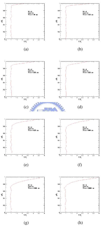
Fig. 3.39 Contours of temperature for M=4, Kn=10 at (a) t =50s; (b) t =125s; (c) t =225s; (d) t =325s; (e) t =425s; (f) t =600s; (g) t =1500s; (h) t =3000s ... 94

Fig. 3.40 Contours of temperature for M=4, Kn=1 at (a) t =40s; (b) t =100s; (c) t =180s; (d) t =320s; (e) t =480s; (f) t =700s; (g) t =1100s; (h) t =1800s ... 95

Fig. 3.41 Contours of temperature for M=4, Kn=0.1 at (a) t =10s; (b) t =50s; (c) t =150s; (d) t =300s; (e) t =500s; (f) t =900s; (g) t =2500s; (h) t

(14)

=4500s ... 96

Fig. 3.42 Contours of temperature for M=4, Kn=0.01 at (a) t =10s; (b) t =75s; (c) t =175s; (d) t =300s; (e) t =500s; (f) t =900s; (g) t =1750s; (h) t =3750s ... 97

Fig. 3.43 Contours of temperature for M=4, Kn=0.0033 at (a) t =10s; (b) t =40s; (c) t =120s; (d) t =400s; (e) t =800s; (f) t =1200s; (g) t =1800s; (h) t =2650s ... 98

Fig. 3.44 Profiles of u-velocity for M=4, Kn=10 along vertical lines through

geometric center (x/L=0.5) at t =50 ~ 3000s. ... 99

Fig. 3.45 Profiles of u-velocity for M=4, Kn=1 along vertical lines through

Fig. 3.46 Profiles of u-velocity for M=4, Kn=0.1 along vertical lines through

Fig. 3.49 Profiles of v-velocity for M=4, Kn=10 along vertical lines through

Fig. 3.50 Profiles of v-velocity for M=4, Kn=1 along vertical lines through

Fig. 3.51 Profiles of v-velocity for M=4, Kn=0.1 along vertical lines through

Fig. 3.54 Profiles of number density for M=4, Kn=10 along vertical lines through

geometric center (x/L=0.5) at =50 ~ 3000s. ... 109

Fig. 3.55 Profiles of number density for M=4, Kn=1 along vertical lines through

Fig. 3.56 Profiles of number density for M=4, Kn=0.1 along vertical lines through

Fig. 3.57 Profiles of number density for M=4, Kn=0.01 along vertical lines through

Fig. 3.58 Profiles of number density for M=4, Kn=0.0033 along vertical lines

through geometric center (x/L=0.5) at t =10 ~ 2600s... 113

(15)

Fig. 3.60 Profiles of temperature for M=4, Kn=1 along vertical lines through

Fig. 3.61 Profiles of temperature for M=4, Kn=0.1 along vertical lines through

Fig. 3.64 Profiles of u-velocity for M=4, Kn=10 along horizontal lines through

geometric center (y/L=0.5) at =50 ~ 3000s. ... 119

Fig. 3.65 Profiles of u-velocity for M=4, Kn=1 along horizontal lines through

geometric center (y/L=0.5) at t =40 ~ 1800s. ... 120

Fig. 3.66 Profiles of u-velocity for M=4, Kn=0.1 along horizontal lines through

Fig. 3.69 Profiles of v-velocity for M=4, Kn=10 along horizontal lines through

Fig. 3.70 Profiles of v-velocity for M=4, Kn=1 along horizontal lines through

Fig. 3.71 Profiles of v-velocity for M=4, Kn=0.1 along horizontal lines through

Fig. 3.74 Profiles of number density for M=4, Kn=10 along horizontal lines through

Fig. 3.76 Profiles of number density for M=4, Kn=0.1 along horizontal lines through

Fig. 3.77 Profiles of number density for M=4, Kn=0.01 along horizontal lines

through geometric center (y/L=0.5) at t =10 ~ 3750s... 132

(16)

through geometric center (y/L=0.5) at t =10 ~ 2600s... 133

Fig. 3.79 Profiles of temperature for M=4, Kn=10 along horizontal lines through

Fig. 3.81 Profiles of temperature for M=4, Kn=0.1 along horizontal lines through

Fig. 3.84 Profiles of u-velocity for M=4, Kn=10 along horizontal lines through upper

wall (y/L=0.9875) at =50 ~ 3000s. ... 139

Fig. 3.85 Profiles of u-velocity for M=4, Kn=1 along horizontal lines through upper

wall (y/L=0.9875) at t =40 ~ 1800s. ... 140

upper wall (y/L=0.9875) at t =10 ~ 4500s. ... 141

Fig. 3.89 Profiles of v-velocity for M=4, Kn=10 along horizontal lines through upper

wall (y/L=0.9875) at =50 ~ 3000s. ... 144

Fig. 3.90 Profiles of v-velocity for M=4, Kn=1 along horizontal lines through upper

wall (y/L=0.9875) at t =40 ~ 1800s. ... 145

upper wall (y/L=0.9875) at =50 ~ 3000s. ... 149

Fig. 3.96 Profiles of number density for M=4, Kn=0.1 along horizontal lines through

(17)

through upper wall (y/L=0.995) at t =10 ~ 3750s. ... 152

Fig. 3.98 Profiles of number density for M=4, Kn=0.0033 along horizontal lines

through upper wall (y/L=0.9983) at t =10 ~ 2600s. ... 153

upper wall (y/L=0.9875) at =50 ~ 3000s. ... 154

Fig. 3.105 Positions of the center of the vortex for M=4, Kn=10 at 1000 ~ 3000s. ... 160

Fig. 3.106 Positions of the center of the vortex for M=4, Kn=1 at 1000 ~ 1800s.160

Fig. 3.107 Positions of the center of the vortex for M=4, Kn=0.1 at 2000 ~ 4500s. ... 161

Fig. 3.108 Positions of the center of the vortex for M=4, Kn=0.01 at 1000 ~ 3750s. ... 161

Fig. 3.109 Positions of the center of the vortex for M=4, Kn=0.0033 at 1200 ~

2600s. ... 162

Fig. 3.110 Positions of the center of the vortex with M=4 for values of x/L and

Knudsen number. ... 163

Fig. 3.111 Positions of the center of the vortex with M=4 for values of y/L and

Knudsen number. ... 163

(18)

Nomenclature

 ：mean free path

 ：density

 ：the differential cross section

 ：viscosity temperature exponent

 : space domain rot  ：rotational energy v  ：vibrational energy rot

 ：rotational degree of freedom

v

 ：vibrational degree of freedom t ：time-step

T ：the total cross section

c ：the total velocity c’ ：random velocity

co ：mean velocity

cr ：relative speed

d ：molecular diameter

D ：the throat diameter of the twin-jet interaction dref ：reference diameter

E ：energy

k ：the Boltzmann constant Kn ：Knudsen number

Knmax : continuum breakdown parameter

. max

Thr

Kn : the threshold value of continuum breakdown parameter

Q

Kn : local Knudsen numbers based on flow property Q L ：characteristic length;

m ：molecule mass

(19)

n ：number density

Tne

P : thermal non-equilibrium indicator

.

Thr Tne

P : the threshold value of thermal non-equilibrium indicator Re ：Reynolds number

To ：stagnation temperature

T ：free-stream temperature

Tref ：reference temperature

Trot ：rotational temperature

Ttot ：total temperature

Ttr ：translational temperature

Tv ：vibrational temperature

Tw ：wall temperature

(20)

Chapter 1 Introduction

1.1. Motivation and Background

1.1.1 Importance of Driven Cavity Flows

The driven cavity flow is one of the fundamental problems in the fluid dynamics. The

kind of topic establishes the foundation of fluid dynamic theory and its geometry simple, but

having singular points at the corners, which may cause difficulties in numerical simulations.

In addition, fluid flows involved in micro-electrical-mechanical devices, vacuum systems, and

high altitude aerodynamics do not have local equilibrium. In these applications, gas flows in

channels, tubes, and ducts due to pressure and temperature gradients in the flow direction are

very common. Several practical applications require understanding of this kind of flows in

detail. However they have been completely studied in the literature, most of researches

focused on incompressible or continuum compressible regime [Karniadakis, 2001] or

compared the geometry type of the cavity and effect on fluid model which based on Reynolds

number is all numerous contribution. Very few researches have been done in the rarefied and

near continuum regimes, where the understanding may become important in micro- and

nano-scale gas flows that are often encountered in MEMS and NEMS related devices. It may

(21)

fails to describe the flow accurately. Therefore, an accurate numerical solution of a driven

cavity flow in the rarefied and near-continuum regime is required.

1.1.2 Classification of Rarefaction

Knudsen number (Kn=/L) is usually used to indicate the degree of rarefaction. Note that

the mean free path  is the average distance traveled by molecules before collision and L is

the flow characteristic length. In general, flows are divided into four regimes and three

solutions. When the local Kn number approaches zero, the flow reaches inviscid limit and can

be solved by Euler equation. As local Kn increases, molecular nature of the gas becomes

dominated. Hence, when the flow is close to the continuum regime (Kn approach 0.01), the

well known Navier-Stokes equation may be applied to yield accurate result for engineering

purposes. For Kn larger than 0.01, continuum assumption begins to break down and the

particle-based method is necessary and a kinetic approach, based on the Boltzmann equation

[Cercignani, 1998]. It is important to note that the kinetic approach is valid in the whole range

of the gas rarefaction. This is an important advantage when systems with multiscale physics

are investigated; however it is rarely used to numerically solve the practical problems because

of two major difficulties. They include higher dimensionality (up to seven) of the Boltzmann

equation and the difficulties of correctly modeling the integral collision term. The well known

direct simulation Monte Carlo (DSMC) method [Bird, 1994] is also a powerful computational

(22)

1.1.3 Direct Simulation Monto Carlo Method

Direct Simulation Monte Carlo (DSMC), was proposed by Bird to solve the Boltzmann

equation using direct simulation of particle collision kinetics, and the associated monograph

was published in 1994 [Bird’s book]. Later on, both Nanbu [1986] and Wagner [1992] were

able to demonstrate mathematically that the DSMC method is equivalent to solving the

Boltzmann equation as the simulated number of particles becomes large. The DSMC method

is a particle method for the simulation of gas flows. The gas is modeled at the microscopic

level using simulated particles, which each represents a large number of physical molecules or

atoms. The physics of the gas are modeled through the motion of particles and collisions

between them. Mass, momentum and energy transports between particles are considered at

the particle level. The method is statistical in nature and depends heavily upon

pseudo-random number sequences for simulation. Physical events such as collisions are

handled probabilistically using largely phenomenological models, which are designed to

reproduce real fluid behavior when examined at the macroscopic level. This method has

become a widely used computational tool for the simulation of gas flows in the transitional

flow regime, in which molecular effects become important.

The DSMC method becomes very time-consuming as the flow approaches continuum

regime since the sampling cell size has to be much smaller than the local mean free path for

(23)

(1) parallel computing [Robinson, 1996-1998]; (2) variable time-step scheme for steady flows

[Kannenberg, 2000]; (3) sub-cells within each sampling cell [Bird’s book, 1994], and (4)

unsteady flows sampling. Details of the “parallel computing”, “variable time-step scheme”

and “sub-cell” can be found in those references cited in the above and are not described here

for brevity. Only “unsteady flows sampling” concept is described here since it was rarely

discussed in detail in the literature. Unsteady flow simulations have difficulties in DSMC

sampling, Cave, et al. [2007] developed new model for under-expanded jets from sonic

nozzles during the start up of rocket nozzles and during the injection phase of the Pulsed

Pressure Chemical Vapor Deposition (PP-CVD) process. But sampling over a small time

interval requires either a very large number of simulated molecules or the average of a large

number of separate simulations (“ensemble-averaging”). The costs high computational

expense and large memory. Xu [1993] used one method of decreasing the statistical scatter of

the results is to using statistical smoothing procedures in two dimensional unsteady problems.

Wagner [1992] proved Bird’s two-dimensional axis-symmetric code which incorporates

unsteady sampling techniques in which a number of time intervals close to the sampling point

are averaged (“time-averaging”); however this is single processor code. The increased

computational capacities of parallel-DSMC techniques have the potential to enable the

simulation of time-dependent flow problems at the near-continuum regime.

(24)

et al., 2007] for transient cavity flow and uses DSMC rapid ensemble averaging method

(DREAM) to reduce the statistical scatter with an acceptable runtime for unsteady flow

simulation.

1.2. Literature Survey

Driven flows are encountered in systems not in equilibrium. Proto-type flows of this kind

are the Couette flow problem in one dimension and the driven cavity flow problem in two or

three dimensions. The Couette flow problem has been studies [Cercignani, 1994]. It is

clarified that in the fluid dynamics, the cavity problem is a well known typical benchmark

problem for testing and verifying continuum solvers and has been thoroughly studied [Hou, et

al., 1995]. However, the research work for the same flow pattern in the free molecular,

transient, and slip regimes is very limited. Recently, the two-dimensional cavity flow problem

was studied using lattice Boltzmann method with slip conditions.

Huang, et al. [2003] validated one dimensional incompressible Couette flow by

Navier-Stokes equations. He used forth Runge-Kutta method and compared with exact

solution. In this thesis, we will also use the result to validate unsteady sampling method. Ghia,

et al. [1982] used the 2D incompressible Navier-Stoke equation to study the laminar

incompressible flow in a square cavity whose top wall moves with a uniform velocity. The

(25)

velocity along vertical and horizontal line through geometry center of cavity and the primary

vortex position. Until very recently, Naris and Valougeorgis [2005] used BGK model to

simulate the driven cavity flow over the whole range of the Knudsen number. They presented

the simulation data over the whole range of the Knudsen number and various aspect ratio

(height/width). However, simulation results by Naris and Valougeorgis [2005] were only

good for low speed rarefied gas flows since the BGK Boltzmann equation was used. In

addition, no data were validated by comparing with experiments or solution from direct

Boltzmann equation, such as DSMC method.

Cave et al., [2007] developed a unsteady sampling procedures for the parallel direction

simulation Monte Carlo method. This paper is simulations of a shock tube and the

development of Couette flow are then carried out as validation studies. To overcome the large

computational expense and memory requirements usually involved in DSMC simulations of

unsteady flows. “Time-averaging” method was implemented which has considerable

computational advantages over ensemble-averaging a large number of separate runs. Also, in

order to reduce the statistical scatter with an acceptable runtime for unsteady flow simulation

using DSMC technique. DSMC-DREAM (Rapid Ensembled Average Method) was

developed whereby a combination of time- and ensemble-averaged data was build up by

regenerating the particle data a short time prior to the sampling point of interesting, assuming

(26)

and validated this code.

1.3. Specific Objectives of the Thesis

The current objectives of the thesis are summarized as follows:

1. To verify of the unsteady sampling and DREAM techniques in a parallelized DSMC

code (PDSC).

2. To verify of the transient sub-cell technique in a parallelized DSMC code (PDSC).

3. To simulate driven cavity flows, including Ma=4 of the speed of top driven plate and

Kn=10-0.0033, based on the average number density and wall temperature.

4. To discuss the effects of Knudsen Number of the driven plate on the flow fields.

The organization of the thesis is stated as follows: Chapter 1 describes the Introduction,

Chapter 2 describes the Numerical Method, Chapter 3 describes the verification of

implementation of unsteady sampling and DREAM techniques, and followed by the

Results and Discussion, and finally Chapter 4 describes the conclusion and

(27)

Chapter 2 Numerical Methods

2.1. The Boltzmann Equation

The Knudsen number (Kn) is used to indicate the degree of rarefaction. In Fig. 2.1, flows

are divided into four regimes and three solutions. We have found the Boltzmann equation is

valid for all flow regimes which from 10 to 0.0001. It is one of the most important transport

equations in non-equilibrium statistical mechanics, which deals with systems far from

thermodynamics equilibrium. There are some assumptions made in the derivation of the

Boltzmann equation which defines limits of applicability. They are summarized as follows:

1. Molecular chaos is assumed which is valid when the intermolecular forces are

short range. It allows the representation of the two particles distribution function

as a product of the two single particle distribution functions.

2. Distribution functions do not change before particle collision. This implies that the

encounter is of short time duration in comparison to the mean free collision time.

3. All collisions are binary collisions.

4. Particles are uninfluenced by intermolecular potentials external to an interaction.

According to these assumptions, the Boltzmann equation is derived and shown as Eq. (2.1)

4 2 ' ' ( ) ( ) ( ) ( ) nf nf nf f u F n f f ff g d dU                 

 

(2.1)

(28)

Meaning of particle phase-space distribution function f is the number of particles with

center of mass located within a small volume d r near the point3 r, and velocity within a range 3

d u , at timet . F is an external force per unit mass and t is the time and _i u is the _i

molecular velocity.  is the differential cross section and d is an element of solid angle. The prime denotes the post-collision quantities and the subscript 1 denotes the collision

partner. Meaning of each term in Eq. (2.1) is described in the following;

1. The first term on the left hand side of the equation represents the time variation of

the distribution function of the particles (unsteady term).

2. The second term gives the spatial variation of the distribution function (flux term).

3. The third term describes the effect of a force on the particles (force term).

4. The term at right hand side of the equation is called the collision integral (collision

term). It is the source of most of the difficulties in obtaining solutions of the

Boltzmann equation.

In general, it is difficult to solve the Boltzmann equation directly using numerical

method because the difficulties of correctly modeling the integral collision term. Instead, the

DSMC method was used to simulated problems involving rarefied gas dynamics, which is the

(29)

2.2. General Description of the standard DSMC

In order to the expected rarefaction caused by the rarefied gas flows, the direct simulation

Monte Carlo (DSMC) method which is a particle-based method developed by Bird during the

1960s and is widely used an efficient technique to simulate rarefied gas regime [Bird, 1976

and Bird, 1994]. In the DSMC method, a large number of particles are generated in the flow

field to represent real physical molecules rather than a mathematical foundation and it has

been proved that the DSMC method is equivalent to solving the Boltzmann equation [Nanbu,

1986 and Wagner, 1992]. The assumptions of molecular chaos and a dilute gas are required

by both the Boltzmann formulation and the DSMC method [Bird, 1976 and Bird, 1994].

An important feature of DSMC is that the molecular motion and the intermolecular collisions

are uncoupled over the time intervals that are much smaller than the mean collision time.

Both the collision between molecules and the interaction between molecules and solid

boundaries are computed on a probabilistic basis and, hence, this method makes extensive use

of random numbers. In most practical applications, the number of simulated molecules is

extremely small compared with the number of real molecules. The general procedures of the

DSMC method are described in the next section, and the consequences of the computational

approximations can be found in Bird [Bird, 1976 and Bird, 1994].

In DSMC, there are three molecular collision models for real physical behavior and imitate

(30)

Variable Soft Sphere (VSS) molecular models, in the standard DSMC method [Bird, 1994].

The collision pairs then are chosen by the acceptance-rejection method. The no time counter

(NTC) method is an efficient method for molecular collision. This method yield the exact

collision rate in both simple gases and gas mixtures, and under either equilibrium or

non-equilibrium conditions.

Fig. 2.2 is a general flowchart of the DSMC method. Important steps of the DSMC method

include setting up the initial conditions, moving all the simulated particles, indexing (or

sorting) all the particles, colliding between particles and sampling the molecules within cells

to determine the macroscopic quantities. The details of each step will be described in the

following;

 Initialization

The first step to use the DSMC method in simulating flows is to set up the geometry and

flow conditions. A physical space is discredited into a network of cells and the domain

boundaries have to be assigned according to the flow conditions. An important feature has to

be noted is the size of the computational cell should be smaller than the mean free path, and

the distance of the molecular movement per time step should be smaller than the cell

dimension. After the data of geometry and flow conditions have been read in the code, the

numbers of each cell is calculated according to the free-stream number density and the current

(31)

Maxwell-Boltzmann distribution according to the free-stream velocities and temperature, and

the positions of each particle are randomly allocated within the cells.

 Molecular Movement

After initialization process, the molecules begin move one by one, and the molecules move

in a straight line over the time step if it did not collide with solid surface. For the standard

DSMC code by Bird [Bird, 1976 and Bird, 1994], the particles are moved in a structured

mesh. There are two possible conditions of the particle movement. First is the particle

movement without interacting with solid wall. The particle location can be easy located

according to the velocity and initial locations of the particle. Second is the case that the

particle collides with solid boundary. The velocity of the particle is determined by the

boundary type. Then, the particle continues its journey from the intersection point on the cell

surface with its new absolute velocity until it stops. Although it is easier to implement by

using structured mesh, it is difficult for those flows with complex geometry.

 Indexing

The location of the particle after movement with respect to the cell is important information

for particle collisions. The relations between particles and cells are reordered according to the

order of the number of particles and cells. Before the collision process, the collision partner

will be chosen by a random method in the current cell. And the number of the collision

(32)

 Gas-Phase Collisions

The other most important phase of the DSMC method is gas phase collision. The current

DSMC method uses the no time counter (NTC) method to determine the correct collision rate

in the collision cells. The number of collision pairs within a cell of volume V over a time C

interval t is calculated by the following equation;

c r T N c t V F N N ( ) / 2 1 max  (2.2) N and N are fluctuating and average number of simulated particles, respectively. F is _N

the particle weight, which is the number of real particles that a simulated particle represents.

T

 and c are the cross section and the relative speed, respectively. The collision for each r

pair is computed with probability

(Tcr)/(Tcr)m a x (2.3)

The collision is accepted if the above value for the pair is greater than a random fraction.

Each cell is treated independently and the collision partners for interactions are chosen at

random, regardless of their positions within the cells. The collision process is described

sequentially as follows:

1. The number of collision pairs is calculated according to the NTC method, Eq. (2.2), for each cell.

(33)

4. The collision is accepted if the computed probability, Eq (2.3), is greater than a random number.

5. If the collision pair is accepted then the post-collision velocities are calculated using the mechanics of elastic collision. If the collision pair is not to collide, continue choosing the next collision pair.

6. If the collision pair is polyatomic gas, the translational and internal energy can be redistributed by the Larsen-Borgnakke model [Borgnakke and Larsen, 1975], which assumes in equilibrium.

The collision process will be finished until all the collision pairs are handled for all cells

and then progress to the next step.

 Sampling

After the particle movement and collision process finish, the particle has updated positions

and velocities. The macroscopic flow properties in each cell are assumed to be constant over

the cell volume and are sampled from the microscopic properties of each particle within the

cell. The macroscopic properties, including density, velocities and temperatures, are

calculated in the following equations [Bird, 1976 and Bird, 1994];

nm   _(2.4a) ' c c c c_o   _o  (2.4b) ) ' ' ' ( 2 1 2 3 2 2 2 w v u m kT_tr    (2.4c)

(34)

) ( 2 r rot rot k T    (2.4d) ) ( 2 v v v k T    (2.4e) ) 3 ( ) 3

( tr rot rot v v rot v tot T T T

T      (2.4f)

n, m are the number density and molecule mass, receptively. c, co, and c’ are the total

velocity, mean velocity, and random velocity, respectively. In addition, Ttr, Trot, Tv and Ttot are

translational, rotational, vibration and total temperature, respectively. rotandvare the

rotational and vibration energy, respectively. rot and v are the number of degree of

freedom of rotation and vibration, respectively.

If the simulated particle is monatomic gas, the translational temperature is regarded simply as

total temperature. Vibration effect can be neglect if the temperature of the flow is low enough.

The flow will be monitored if steady state is reached. If the flow is under unsteady

situation, the sampling of the properties should be reset until the flow reaches steady state.

As a rule of thumb, the sampling of particles starts when the number of molecules in the

calculation domain becomes approximately constant.

2.3. General Description of the PDSC

Although the large number of molecules in a real gas is replaced with a reduced number

of model particles, there are still a large number of particles must be simulated, leading to

tremendous computer power requirements and needing to cost a lot of computational time. As

(35)

simplified flow chart of the parallel DSMC method used in the current study. The DSMC

algorithm is readily parallelized through physical domain decomposition. The cells of the

computational grid are distributed among the processors. Each processor executes the DSMC

algorithm in serial for all particles and cells in its domain. Data communication occurs when

particles cross the domain (processor) boundaries and are then transferred between

processors.

Parallel DSMC Code (PDSC) is the main solver used in this thesis, which utilizes

unstructured tetrahedral mesh. Fig. 2.4 is the features of PDSC and brief introduction is listed

in the following paragraphs.

1. 2D/2D-axisymmetric/3-D unstructured-grid topology: PDSC can accept either

2D/2D-axisymmetric (triangular, quadrilateral or hybrid triangular-quadrilateral) or 3D (tetrahedral, hexahedral or hybrid tetrahedral-hexahedral) mesh [Wu et al.’s JCP paper, 2006]. Computational cost of particle tracking for the unstructured mesh is generally higher than that for the structured mesh. However, the use of the unstructured mesh, which provides excellent flexibility of handling boundary conditions with complicated geometry and of parallel computing using dynamic domain decomposition based on load balancing, is highly justified.

2. Parallel computing using dynamic domain decomposition: Load balancing of PDSC

is achieved by repeatedly repartitioning the computational domain using a multi-level graph-partitioning tool, PMETIS [Wu and Tseng, 2005] by taking advantage of the unstructured mesh topology employed in the code. A decision policy for repartition with a concept of Stop-At-Rise (SAR) [Wu and Tseng, 2005]

(36)

or constant period of time (fixed number of time steps) can be used to decide when to repartition the domain. Capability of repartitioning of the domain at constant or variable time interval is also provided in PDSC. Resulting parallel performance is excellent if the problem size is comparably large. Details can be found in Wu and Tseng [Wu and Tseng, 2005].

3. Spatial variable time-step scheme: PDSC employs a spatial variable time-step

scheme (or equivalently a variable cell-weighting scheme), based on particle flux (mass, momentum, energy) conservation when particles pass interface between cells. This strategy can greatly reduce both the number of iterations towards the steady state, and the required number of simulated particles for an acceptable statistical uncertainty. Past experience shows this scheme is very effective when coupled with an adaptive mesh refinement technique [Wu et al.’s CPC paper, 2004].

4. Unsteady flow simulation: An unsteady sampling routine is implemented in PDSC,

allowing the simulation of time-dependent flow problems in the near continuum range [JCP paper submitted in June 2007]. A post-processing procedure called DSMC Rapid Ensemble Averaging Method (DREAM) is developed to improve the statistical scatter in the results while minimizing both memory and simulation time. In addition, a temporal variable time-step (TVTS) scheme is also developed to speed up the unsteady flow simulation using PDSC. More details can be found in [JCP paper submitted in June 2007]. Details of the idea and implementation are described next.

5. Transient Sub-cells: Recently, transient sub-cells are implemented in PDSC directly

on the unstructured grid, in which the nearest-neighbor collision can be enforced, whilst maintaining minimal computational overhead [JFM paper under preparation,

(37)

2.4.

General Description of Unsteady Sampling Method in DSMC

[JCP

paper submitted in June 2007]

In section 2.3, the PDSC code has been specifically designed for simulating steady flows,

therefore some modification is need for unsteady sampling. The unsteady sampling method

has been described in detail in the paper [Cave, et al., 2007].

There are two methods for unsteady sampling, the differences illustrated in Fig. 2.5

and the details will be described in the following;

1. The “Ensemble-Average” method, require multiple simulation runs. The flow flied is sampled at the suitable sampling times during the run. The sampling simulation outputs from each run are averaged over the runs. There the results are vary precise, but the method is very computational expensive. Because a large of runs is required to reduce the statistical scatter to smooth data and a large amount of memory is needed to record the sampling data for each simulation.

2. The “Time-Average” method, require one simulation run. It averages a number of time steps over an interval before the sampling time. However it suffers a potential disadvantage in that the results will be “smeared” over the time over which samples are taken. Hence the sample time must be sufficiently short to minimizes time “smearing” and yet long enough to obtain a good statistical sample. This method of time averaging has been used previously by Auld to model shock tube flow [Auld, 1992]

(38)

shows the flow chart of the PDSC method with the unsteady sampling procedures

implemented. Here M is the output matrix for sampling interval M. Most parts of the

procedure are the same as the steady simulation except the sampling data must be reset after

completing each simulation interval.

2.5.

DSMC Rapid Ensemble Averaging Method (DREAM)

[JCP paper

submitted in June 2007]

Because reducing the statistical scatter greatly, in time-average data requires a very large

number of simulation particles with consequent large computational times. In the thesis, we

have adapted DREAM code which has been described in detail in this paper by [Cave, et al.,

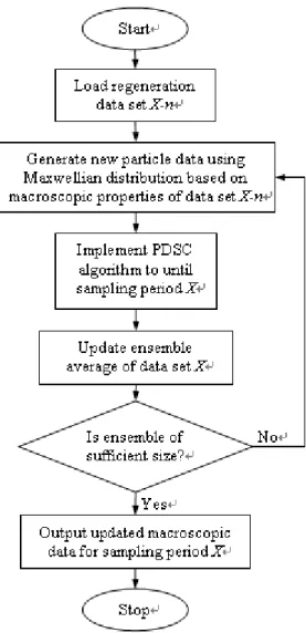
2007]. The illustrated in Fig. 2.7

First, we select a raw data set X-n produced by PDSC n sampling intervals prior to the

sampling interval of interest X. New particle data is generated from the macroscopic

properties in data set X-n by assuming a Maxwellian distribution of velocities. The standard

PDSC algorithm is then used to simulate forward in time until the sampling period of interest

X is reached. The time steps close to the sampling point are time-averaged in the same way as

in PDSC and this process is repeated a number of times, thus building up a combination of

ensemble-averaged and time-averaged data without having to simulate from zero flow time

(39)

of particles in the sample, rather than by some artificial smoothing process. Because only a

short period of the flow is processed in this way, the scheme has significant memory and

computational advantages over both ensemble-averaging and using a greater number of

(40)

Chapter 3 Results and Discussion

3.1. Quasi 1-D Couette Flows

Although this thesis is concerned with supersonic square driven cavity flows in rarefied

regime, a subsonic flow case with M=0.3 and Kn=0.02 is used as the benchmark case. The

rationale is that a subsonic flow represents a more stringent test problem than a supersonic

flow for the DSMC method in terms of statistical uncertainties. Flow and simulation

conditions are summarized in Table 1. The validation process is described sequentially as

follows:

First, as a validation of the unsteady sampling techniques in the PDSC code, we have

used the test problem of quasi 1-D Couette flows. We have adapted Huang’s paper [[2003]].

The simulation results of a quasi-1D incompressible Couette flow with the analytical data.

Second, use DREAM techniques [Cave, et al., 2007] and simulate the same conditions in

the PDSC code which compare the result.

Third, as a validation of transient sub-cell techniques in the PDSC code, we have use the different x_ and try to find optimal x_ .

(41)

3.1.1. Problem Description and Test Conditions

The computational domain for this simulation is shown in Fig. 3.1. Although this

problem is quasi 1-D, we used 100 x 100 cell was used to validate the code. This grid spacing

was chosen to be half of the mean free path in the undisturbed gas. The mesh is show in Fig.

3.2. Here argon gas is initially at rest between two parallel diffuse plates at the same uniform

temperature as the gas, in this case 300K. At time t=0 the upper plate begins moving

instantaneously at speed U∞=96.6 m/s. These conditions correspond to a Mach 0.3 flow with a

Knudsen number of 0.02. The simulation time step was set at 3.11x10-5s and used 100

sampling times.

In Huang’s paper [2003], a continuum solution for the velocity at the vertical position y

and time t can be obtained from the incompressible Navier-Stokes equations:

 

















          0 0 1 1 2 1 2 , n n n erfc n erfc U t y U _ _ _ _ (3-1)

where   y 2 t , ₁  H 2 t, erfc is the complementary error function and v is the kinematics viscosity.

3.1.2. Verifications of Unsteady Sample Method

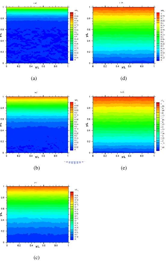
Fig. 3.3 (a)-(e) shows the velocity contour from the DSMC data on normalized time from

t =1 to t =36, in all cases time has been normalized such that t = t*U∞/L., where t* is real time,

(42)

plate speed and length (also width) of the driven cavity, respectively. The upper plate

suddenly starts the velocity and conducts kinetic energy to lower plate gradually. However,

the DSMC data exhibit the statistical scatter with an acceptable runtime for unsteady flow

simulation.

Compare Huang’s paper [2003] which introduces Couette flow exact solution. Fig. 3.4

shows the u-velocity profiles along the x/L=0.5 line for a number of flow times as the Couette

flow developed. Result show that lines (analytical in compressible Navier- Stokes solution)

close to symbol point from DSMC data approximately, but the DSMC solution lags the

incompressible continuum solution. This is because the high level of rarefaction effectively

results in slip between gas particles and the walls.

3.1.3. Verifications of DSMC Rapid Ensemble Average Method (DREAM)

In order to reduce the statistical scatter for unsteady flow simulation, use DSMC Rapid

Ensemble Average Method [Cave, et al., 2007]. Fig. 3.5 (a)-(e) shows the velocity contour

from the DREAM data on normalized time from t =1 to t =36. Result show that the DREAM

can greatly reduce the statistical scatter for unsteady flow simulation using DSMC technique.

Fig. 3.6 (a)-(e) shows a comparison of the velocity profile from the unsteady DSMC data and

the data after processing by DREAM as the flow from t =1 to t =32, illustrating the reduction

(43)

number of flow times as the Couette flow developed. All data has been processed by

DREAM and also exhibits the expected phenomenon of velocity slip at the walls.

3.1.4. Benchmark of the Transient Sub-Cell Method

In the section, obtain optimal sub-cell [Tesng, et al., 2007] to allow the maintenance of

good collision quality within the simulation. Even for grids which are “under-resolved” (that

is, if the sampling cells are bigger than the recommended setting of 1/3 ~ 1 times the local

mean free path). Running simulations with under-resolved sampling cells which employ

sub-cells results in a reduction in the computational and memory requirements of the

simulation, albeit at the cost of a reduction in the possible sampling resolution of the

macroscopic properties, but without sacrificing simulation accuracy. In order to obtain

optimal and verification, compare coarse mesh with transient sub-cell with finer mesh without

transient sub-cell.

First, use finer mesh to simulate Couette flow. These conditions correspond to a Mach

0.3 flow with a Knudsen number of 0.02. The mesh for this simulation is shown in Fig. 3.8. This grid spacing was chosen to be x y

 

 

 =0.25 and the domain 1m x 0.025m. Here argon gas is initially at rest between two parallel diffuse plates at the same uniform temperature as

the gas, in this case 300K. At time t=0 the upper plate begins moving instantaneously at

(44)

times. Fig 3.9 shows the velocity contour on normalized time from t =7. The data has been

processed by DREAM. Fig. 3.10 shows the merit of collision (=mean collision distance/local

mean free path), which represents the quality of collisions in a DSMC simulation. The

average data is about 0.12; this is good for collision in each cell.

Second, use coarse mesh to simulate Couette flow. These conditions correspond to a

Mach 0.3 flow with a Knudsen number of 0.02. The mesh for this simulation is shown in Fig.

3.11. This grid spacing was chosen to be x y

 

 

 =1 and the domain 1m x 0.1m. Here argon gas is initially at rest between two parallel diffuse plates at the same uniform temperature as

the gas, in this case 300K. At time t=0 the upper plate begins moving instantaneously at speed

U∞=96.6 m/s. The simulation time step was set at 3.11x10-5s and used 100 sampling times.

Fig. 3.12 shows the velocity contour on normalized time from t =7. The data has been

processed by DREAM. Fig. 3.13 shows the merit of collision (=mean collision distance/local

mean free path), which represents the quality of collisions in a DSMC simulation. The

average data is about 0.15; this is good for collision in each cell. Finally, compare these results. Fig. 3.14 shows the x y

     =0.25 simulation compare to x y    

 =1. Result show the simulation used coarse mesh with transient sub-cell approximate that used finer mesh without transient sub-cell. In addition, result with transient

sub-cell could improve near lower plate effect. Therefore, the simulation with transient

(45)

but still has simulation accuracy.

3.2. Instantaneously Started Driven Cavity Flows

According to previous section, result show that the DREAM can greatly reduce the

statistical scatter with an acceptable runtime for unsteady flow simulation using DSMC

technique. Future, the transient sub-cell method can greatly reduce the computational cost and

still has good quality of solution. In this section, we have used this benchmark and to simulate

instantaneously started driven cavity flows in a systematic way. Thus, the result can

understand more about the effects of rarefaction and compressibility in such conditions.

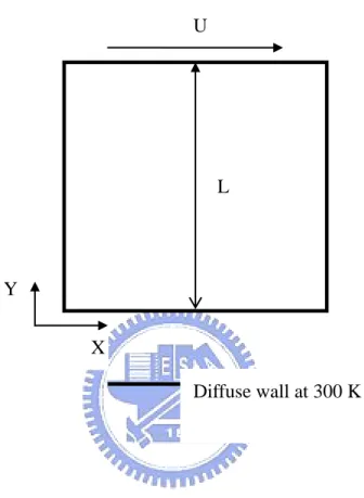
3.2.1. Problem Description and Test Conditions

Fig. 3.15 sketch of the 2D square (L/H=1) driven cavity flow with moving top plate.

Initially, we use argon gas at rest inside the cavity and at the same uniform temperature 300K.

At time t =0 the upper plate begins moving instantaneously at speed Ma=4 and Kn=10-0.0033

based on the mean free path of wall temperature and size of the cavity. Table I shows the grid

sizes of these cases. This grid spacing was chosen to be equal of the mean free path for

Kn=0.01, 0.0033, others cases are setting 40 x 40. The mesh in Knudsen number 10, 1, 0.1

was 40 x 40 showed in Fig. 3.16. The mesh in Knudsen number 0.01 was 100 x 100 showed

(46)

Particle per cell are 100, 100, 25, 25, 25 with Knudsen number 0.0033, 0.01, 0.1, 1, 10. Table

III shows the time step of these cases. The simulation time step was correspond in Knudsen

number, the speed of the top driven plate and the sampling times. All cases use 50 sampling

times

3.2.2. Effects of Knudsen Number

In this section, we were observed effects of Knudsen number in the same Mach number

(Ma=4). First, we were showed general simulation results include u-direction, v-direction,

Mach number, temperature, density and streamline. Second, we were showed property

distributions across cavity geometric center for x/L =0.5m, y/L= 0 to 1m and y/L=0.5m,

x/L=0 to 1m. Third, we showed property distributions near the solid walls. Finally, we were

observed the recirculation center position in different cases.

3.2.2.1. General Simulation Results

3.2.2.1.1. Supersonic Moving Plate (M=4)

Fig. 3.19 - Fig. 3.23 (a)-(h) show that u-velocity contour during started driven upper

plate to steady state for Ma=4, and Knudsen number 10, 1, 0.1, 0.01 and 0.0033 respectively.

In these figures, up and L represents the top plate speed and length (also width) of the driven

使用平行化直接模擬蒙地卡羅法初步模擬在稀薄流體範圍時瞬間啟動的空穴超音速流場

國 立 交 通 大 學

機

械

工

程

學

系

碩士論文

使用平行化直接模擬蒙地卡羅法初步模擬在稀薄流體

範圍時瞬間啟動的空穴超音速流場

Preliminary Simulation of Instantaneously Started

Supersonic Driven Cavity Flows in the Rarefied Gas

Regimes Using the Parallel Direct Simulation Monte Carlo

Method

研 究 生：洪維呈

指導教授：吳宗信 博士

使用平行化直接模擬蒙地卡羅法初步模擬在稀薄流體範圍時瞬間啟動的空

穴超音速流場

Preliminary Simulation of Instantaneously Started Supersonic Driven Cavity

Flows in the Rarefied Gas Regime Using the Parallel Direct Simulation Monte

Carlo Method

研 究 生：洪維呈 Student: Wei-Cheng Hung

指導教授：吳宗信 博士 Advisor: Dr. Jong-Shinn Wu

國立交通大學

機械工程學系

碩 士 論 文

A Thesis

Submitted to Institute of Mechanical Engineering

College of Engineering

National Chiao Tung University

in partial Fulfillment of the Requirements

for the Degree of

Master of Science

in

Mechanical Engineering

July 2007

Hsinchu, Taiwan

中華民國九十六年七月

致謝

使用平行化直接模擬蒙地卡羅法初步模擬在稀薄流體範圍時瞬間

啟動的空穴超音速流場

學生: 洪維呈 指導教授: 吳宗信

國立交通大學機械工程學系

摘要

Preliminary Simulation of Instantaneously Started Supersonic Driven

Cavity Flows in the Rarefied Gas Regime Using the Parallel Direct

Simulation Monte Carlo Method

Student: Wei-Cheng Hung Advisor: Dr. Jong-Shinn Wu

Department of Mechanical Engineering

National Chiao-Tung University

Abstract

Table of Contents

List of Tables

List of Figures

Nomenclature

Chapter 1

Introduction

1.1. Motivation and Background

1.1.1 Importance of Driven Cavity Flows

1.1.2 Classification of Rarefaction

1.1.3 Direct Simulation Monto Carlo Method

1.2. Literature Survey

1.3. Specific Objectives of the Thesis

Chapter 2

Numerical Methods

2.1.

The Boltzmann Equation

 

2.2.

General Description of the standard DSMC

2.3.

General Description of the PDSC

General Description of Unsteady Sampling Method in DSMC

DSMC Rapid Ensemble Averaging Method (DREAM)

Chapter 3

Results and Discussion

3.1. Quasi 1-D Couette Flows

3.1.1. Problem Description and Test Conditions

 

國立交通大學

研究生：洪維呈

指導教授：吳宗信博士

研究生：洪維呈 Student: Wei-Cheng Hung

指導教授：吳宗信博士 Advisor: Dr. Jong-Shinn Wu

碩士論文

學生: 洪維呈指導教授: 吳宗信