接 受 函
周教授治邦道鑒: 恭禧台端之大作「外部性與最適財產稅-實質選擇權模型在不動產投資的應 用」經二位匿名評審之審查並推薦後,本刊決定接受刊登。 請您就下列四點作最後修正。 1.論文格式請參照隨文附上財務金融學刊文稿格式,請依照格式修改(請您 留意參考文獻之格式),並請於2007 年 2 月 6 日前寄回兩份原稿、電腦 磁片及版權移轉聲明書(中、英文稿請以 word 7.0 處理),以便排版作業。2.為求統一,中文字請以標楷體,英文、數字、公式以 Times New Roman 字 型修改。並請書寫中、英文論文題目、關鍵字、中文(300 字)英文(700 字)摘要,註明 email 帳號,英文地址,電話以及傳真。 3.為求讀者之閱讀方便,請將圖表放置於文中(若磁片無法修改請標示適當 位置,並附上清析圖表)。 4.若為英文稿件請作者先把文稿送經專業 edit 後,再將修正稿及磁片寄回。 感謝您的投稿,希望日後能繼續看到您的大作。若有任何問題,請與本刊助 理李雁雯、林韋君聯繫,E-mail: [email protected]。謝謝! 敬 頌 研 安 財務金融學刊總編輯 李 存 修 敬上 2007 年 2 月 6 日
外部性與最適財產稅-實質選擇權模型在不動產投資的應用
*Externality and Optimal Property Taxation:
Application of the Real Options Model to Real Estate Investment
周治邦**
Jyh-Bang Jou National Taiwan University
台灣大學 李丹 Tan Lee Yuan Ze University 元智大學
摘 要
本論文建構一實質選擇權模型,探討政府如何針對房地產廠商開發土地「之前」及「之 後」來課徵最適的財產税。假設房地產產業內有固定家數廠商,在供需均具不確定性的情況 下進行土地開發,且開發耗費成本完全無法回復。當廠商開發面積愈大,會減少綠地面積, 因而對居民不利。然而,土地持有者會忽視此一負面外部性,因而其開發密度會高於社會最 適水準。政府可在房地產廠商開發「之前」及「之後」分別課徵財產稅以矯正此狀況。本模 型的結果顯示,雖然廠商開發土地後才造成負面外部性,但最適的「開發後」稅率不一定要 高於「開發前」的稅率。 關鍵詞:開發密度、負面外部性、財產稅、實質選擇權Abstract
This article investigates the design of property taxation both before and after development in a real options framework where a fixed number of landowners irreversibly develop property in an uncertain environment. We assume that densely developed properties reduce open space, and thereby harm urban residents. However, landowners will ignore this negative externality, and will thus develop properties more densely than is socially optimal. The regulator can correct this tendency by imposing taxation on property both before and after development. It is, however, unclear whether the latter should be taxed at a higher rate than the former even though the negative externality arises only after the property is developed.
Keywords: Development Density, Negative Externality, Property Taxation, Real Options.
* 作者感謝李存修總編輯以及兩位審查及推薦本文之匿名評審。此外,作者亦感謝於年會宣讀時之評論人黃慶
堂教授,於 2006 Joint AsRES-AREUEA 年會宣讀時之評論人 David Ho Kim Hin 教授,以及 Richard Arnott, John Clapp, 與 Charles Leung 等教授所提供的寶貴意見。最後,特別感謝國科會所提供的研究計畫財務補助 (計畫 編號:NSC 95-2416-H-002-045)。
** Tel: (886-2) 33663331 Fax: (886-2) 23679684 Address correspondence to: Professor Jyh-bang Jou, Graduate
1
Externality and Optimal Property Taxation
I. Introduction
The issue regarding the relationship between property taxation and choices over the timing and density of development has recently received widespread attention in studies on real estate economics. However, most of these studies investigate the positive aspect of property taxation, i.e., they examine how these two choices are affected by property taxation. Rarely have studies attempted to discuss the normative aspect of property taxation. Few studies, for instance, ask why the regulator uses property taxation in the first place? To our knowledge, the only theoretical article focusing on this issue is that by Anderson (1993).
Anderson constructs a model in which an owner of vacant land extends benefits to urban residents through the provision of open space. He models this external benefit as an increasing function of the cash inflow received by the owner. Anderson then shows that the regulator can correct the externality through the use of a Pigouvian subsidy to the owner, which should be provided at a rate equal to the ratio of the open space externality during the period of development to the value of the developed land in that period.
Like Anderson, this article also investigates the issue regarding the design of the Pigouvian taxes to correct market inefficiencies in the real estate market. This article, however, differs significantly from Anderson in the following two respects. First, this article explicitly derives the private and social values of the cash flow of the developed properties that exhibit negative externalities from congestion. Second, this article considers a landowner who simultaneously chooses the timing and scale of development. Consequently, to align these two choices of the landowner with those of the central planner, the regulator needs to impose two kinds of policy instruments, such as taxation both before and after development. By contrast, Anderson assumes that a landowner chooses only the timing of development, and thus he considers either the property subsidy before development (when an open space externality exists) or property taxation after development (when a congestion externality exists), but not both.
This article considers a real estate industry that consists of homogeneous landowners and renters. We assume that densely developed properties reduce open space, and thereby harm urban residents. However, no one cares who are actually providing these properties. In order to characterize this aggregate consumption–production externality (Tresch, 2002),1 we assume that renters will pay lower rents if property is developed at a higher density. Landowners will ignore this externality, and will thus develop property at a higher density than is socially optimal. The regulator can correct this tendency by imposing taxation on property both before and after development. It is, however, unclear whether the latter should be taxed at a higher rate than the former even though the negative externality arises only after property is developed.
This article is closely related to the literature on real estate economics that investigates how
1 See Laffont (1998, pp. 193-200) who provides an example regarding the relationship between the
property taxation affects choices concerning the timing and scale of development in a framework where no uncertainty arises. Shoup (1970) is the first paper that investigates the optimal timing of land development. Arnott and Lewis (1979) later investigate the simultaneous choices regarding the timing and density of land development. Skouras (1978) provides an early analysis indicating that property taxation is non–neutral in its effect on the timing of land development. Mills (1983) further introduces property taxation in a model of competitive equilibrium and investigates the timing effects of taxation on land development. By contrast, Anderson (1986) focuses on how property taxation affects the timing decision of land development. Turnbull (1988b) and McFarlane (1999) further investigate how property taxation affects the choices regarding the timing and density of development. These effects, however, largely depend on the assumption regarding how the demanded density is increasing or decreasing over time (see, e.g., Turnbull, 1988a). Our results are in line with those of the case where the demanded density is increasing over time.
Our results are not, however, fully in line with those of Capozza and Li (1994) who also employ a real options model to investigate the timing and intensity decision of a landowner. Capozza and Li assume that the scale developed by a landowner is of a Cobb–Douglas functional form in land and capital, which implies the same cost functional form as ours. They also assume that the rent per unit of developed property is unrelated to the scale of developed property, which is a polar case of our framework. The key departure from our article is that they assume that the rent per unit of developed property follows an arithmetic Brownian motion, while we assume that it is driven by a geometric Brownian motion. With this departure, they find that an increase in the property–tax on undeveloped land accelerates development and reduces the capital intensity (and thus the development density), which is in line with our results. However, they find that an increase in the property–tax on developed land delays expected developed time and reduces capital intensity. The former is in line with our result, while the latter has just the opposite effect. With uniform tax rates on property both before and after development, they find that an increase in the tax rate accelerates development and reduces capital intensity. The former is not in line, while the latter is in line with our results.
The remainder of this article is organized as follows. Section II presents the basic model. Section III solves choices regarding the timing and density of development for both the decentralized and the centralized economy. We investigate how taxation before and after development affects these two choices in the case of the decentralized economy. We also provide the conditions under which the regulator is able to avoid the long run overbuilding problem when imposing these two kinds of taxation. Section IV shows the comparative statics results regarding how various exogenous forces affect the optimal taxation on property both before and after development. Section V concludes by offering testable implications.
II. The Model
Consider a real estate industry that is composed of N identical risk–neutral landowners. Suppose that at date t0 this industry has undeveloped land that is normalized at one unit. At
3
any time, i.e. t0, landowner i (i1,,N) is able to develop property at a scale equal to q ,i and thus at a density equal to Nq , given that each landowner hasi 1 N units of undeveloped land. We also assume that the development cost for landowner i, which is fully irreversible, is equal to (see, e.g., Quigg, 1993; Williams, 1991)2
1 1
( ( ), i) ( ) i ,
C x t q x t q (1)
where x t1( ) is a disturbance term that captures supply shocks, such as unexpected changes in weather or labor market conditions. We allow the housing production technology to be either increasing (1), constant (1), or decreasing (1) returns to scale.
We assume that the rent per unit of developed property is given by
1 2
( ) ( ) b a,
R t x t Q S 1 b a 0, (2)
where x t2( ) denotes the macroeconomic shock from the demand side, Q is the aggregate
demand for developed property, and
1 N i i S q
is the aggregate supply of developed property, which is also equal to the average density of development, given that the industry initially has one unit of undeveloped land. In equation (2), we assume that the rent per unit of developed property will be affected by two different measures of the scale of developed property. First, we assume a non-positive internal effect of Q on R t( ), i.e. the rent per unit of developed property is non-increasing with the scale of developed property. This captures the standard non-positive price-quantity relationship in a demand function. Second, we assume a negative external effect of S on R t( ) with a size measured by coefficient a ; we call this effect external because the utility of a renter will be lower as the aggregate supply of developed property is higher.3 However, no renters can have an appreciable effect on S, and therefore, all renters will take the external effect as exogenously given when deciding whether to rent developed property. We also assume that ba to ensure that landowner i’s total rent, i.e. q R t , will be increasing with the scale ofi ( ) developed property, but at a decreasing rate.Both the supply shock, x t , and the demand shock,1( ) x t , follow geometric Brownian2( ) motions given by
( ) ( ) ( ) ( ),
i i i i i i
dx t x t dtx t d t (3)
where i1, 2. Each variable x ti( ) has a constant expected rate of growth and a constanti variance of the growth rate . Eachi2 di( )t is an increment to a standard Wiener process,
2
McFarlane (1999) argues that investment on land development will be fully irreversible if demolition costs are extremely high. Similarly, Riddiough (1997) suggests that irreversibility is a reasonable assumption with real estate in which the physical asset is long-lived and switching costs to alternative uses are quite high. Turnbull (2005) argues that the irreversibility assumption may be not realistic, but provides analytically tractable solutions.
3
with E d{ i( )}t ,0 E d{ i( )}t 2 , anddt E d( 1( )t d2( ))t , wherer12 1 2dt .1 r12 1 We assume that an individual landowner chooses the timing and scale of development, assuming that the others’decisions as exogenously determined. Consequently, the market outcome will be inefficient. The policy to be adopted to correct this includes density restrictions, or price controls such as property taxes, building fees, and entitlement fees. We focus on property taxes and abstract from the other instruments. We will assume that property taxes before and after development are denoted by andb , respectively.a 4 By following the literature that applies non–cooperative dynamic games to environmental management (see, e.g., Jou 2001, 2004), we model these two kinds of taxation as a hierarchical game. At the lower level of the game, landowners compete for the choice of the date and scale of land development in a Cournot-Nash environment. At the upper level is a Stackelberg game in which the regulator acts as the leader and a landowner acts as the follower. The regulator should anticipate the timing and scale chosen by the landowner, and then set these two kinds of taxation to induce the landowner to make these two choices at the socially optimal level accordingly.
We assume that the risk-less rate of interest is constant per unit of time and that the undeveloped property per unit has a constant positive return given by net cash inflow per unit of time x t2( ). We further assume that 0, an assumption implying that a landowner has no option value to abandon the undeveloped property. We also abstract from both the time-to-build problem that usually occurs in the real estate industry (see, e.g., Bar–Ilan and Strange, 1996; Grenadier, 2000), and the redevelopment problem addressed in Williams (1997). Consequently, in what follows, each landowner as well as the central planner will make his respective development decisions once and for all. Our simplified assumptions may be not so realistic, yet they help us gain insights regarding the determinants of optimal property taxation.
III. Choices of the Date and the Density of Development
Without risk of confusions, we use x t1( ) andx1 x t2( )x2 in what follows. Consider any t after land is developed. Given that redevelopment is prohibited, the value of developed property is equal to the time t expected present value of the future cash flow given by
( )
2 2
( , , ) [ ( ) ( ( ), , )] s t ,
a i t t i a a i
W x Q q E
q R s W x s Q q e ds (4) where q R si ( ) is the cash inflow for landowner i at instant s , which is derived by multiplying the rent per unit of developed property, R(s) in equation (2), by the scale of developed property he owns, q .i Equation (4) can be rewritten as54
Here and in what follows, we use subscripts “a”and “b”to represent “after”and “before”development, respectively.
5 Here and in what follows, we assume that
2
a and b2 so as to ensure that Wa() given by equation (4’)and Wb() given by equation (5) are both finite.
5 1 ( ) 2 2 2 ( , , ) ( ) . ( ) a b a s i a i t t i a q x Q S W x Q q E q R s e ds
(4’)Denote T as the date at which vacant land is developed. Define W x x T qb( ,1 2, , i) as the value of vacant land of a landowner who faces the tax rate from time t to T, which is thus given by
1 2 ( ) 2 1 2 1 ( ) ( ) 2 2 1 ( , , , ) ( ) { ( ( ( ), ( ), , )) ( ( ) ( ( ), , )) ( ) }. b i T s t t t b b i b a s t T t i a a a i i T W x x T q x s E W x s x s T q e ds N q x s Q S W x s Q q e ds x T q e
(5)Equation (5) indicates that the expected present value of returns to the vacant land is the sum of the after-tax expected present value of rents received until time T and the after–tax expected present value of land rent beginning at the time of development, less the expected present value of the development costs. Following Anderson (1993b), Capozza and Li (1994), and McFarlane (1999), a more tractable expression for the value of vacant land is given by
( ) ( )( ) 1 ( )( ) 2 1 2 2 1 ( ) ( , , , ) { T b b T t [ ( ) b a a s T ( ) ]}. b i t t T i i x s W x x T q E e ds e q x s Q S e ds x T q N
(6)Equation (6) can be further written as
1 2 1 2 1 2 ( , , , ) ( , , , ) ( , , , ), b i b i d i W x x T q W x x q V x x T q (7) where 2 1 2 2 ( , , , ) ( ) b i b x W x x q N (8) 1 2 ( )( ) 1 ( )( ) 2 ( )( ) 2 1 ( , , , ) ( ) { b [ ( ) a b ( ) ]}. d i T t b a s T s T t T i T i V x x T q x s E e q x s Q S e ds e ds x T q N
(9)In equation (7), the first term on the right–hand side is the value of vacant land if undeveloped forever, i.e., W x xb( ,1 2, ,qi). Landowner i needs to choose an appropriate timing T and density q to maximize the value of the vacant land.i This is defined as
1 2 1 2 , ( , ) max ( , , , ) i d d i T q Z x x V x x T q , (10)
subject to the evolution of x t1( ) and x t2( ) defined in equation (3).6 In equation (10),
1 2
( , )
d
Z x x is the net value of a perpetual warrant to exchange the fixed q units of developedi
6
The problem of maximizing Wb() in equation (7) is equivalent to that of maximizing Vd() because the first term
on the right-hand side of equation (7) is unrelated to either T or qi. Furthermore, here and in what follows, we use subscript “d”to represent “the decentralized economy.”
properties for 1/ N units of vacant land.
Define Wd( ,x x1 2) as the intrinsic value of the warrant if exercised at time t . Substituting T t into equation (9) yields its value as given by
1 2 2 1 2 1 ( , ) max ( , , ) ( , , , ) i d a i b i i q W x x W x Q q W x x q x q, (11)where the term in braces are the value of developed properties, W x Q qa( 2, , i), minus the opportunity costs of obtaining it, namely, the value of vacant land if undeveloped forever,
1 2
( , , , )
b i
W x x q , and the costs of development, x q1 i. To maximize the intrinsic value at time t , the optimal scale of development, denoted by q , must satisfy the first–d order condition for q :i
( 2, , ) 1
0 a i i i W x Q q x q q , (12)which says that at the optimal scale of development, the expected marginal benefit of an additional scale of development must be equal to the marginal cost of developing it. Given that the intrinsic value of the warrant, if exercised at the optimal exercise date T , may be denoted by
1 2
( ( ), ( ))
d
W x T x T , we can rewrite equation (10) as
( )
1 2 1 2 ( , ) max T t ( ( ), ( )) d t d T Z x x E e W x T x T . (13)The solution for Zd( ,x x1 2) must satisfy the fundamental differential equation of optimal stopping given by 2 2 2 2 2 2 2 1 1 2 12 1 2 1 2 2 2 2 1 2 1 2 ( ) ( ) ( ) 1 1 2 2 d d d Z Z Z x r x x x x x x x (14) 1 1 2 2 1 2 ( ) ( ) ( ) 0. d d d Z Z x x Z x x
The solution to equation (14) is given by
1 1 1 2 1 2
1 2 1 2 1 2 2 1
( , ) d d d d
d d d
Z x x A x x A x x , (15)
where A1d and A2d are constants to be determined, and ,1d , and the overall volatility,2d denoted by , are respectively equal to2
2 1 2 1 2 1 1 2 2 2 2( ) ( ) ( ) 1 1 ( ) 2 2 b d , (16) 2 1 2 1 2 1 2 2 2 2 2( ) ( ) ( ) 1 1 ( ) 2 2 b d , 2 2 2 1 2r12 1 2 2 .
7
Landowner i simultaneously chooses the timing and scale of development. As indicated by Dixit and Pindyck (1994, p.139), when uncertainty arises, we are unable to determine a non-stochastic timing. Instead, the development rule takes the form where landowner i will not develop until the supply shock, x , declines to a certain level, denoted by1 x , and the1d demand shock, x , rises to another level, denoted by2 x2d. When these two trigger levels are reached, landowner i will develop vacant land at a scale denoted by q .d The two critical levels, x1d and x2d , together with A1d and A2d in equation (15), are solved from the boundary conditions given by
2 1 2 0 lim d( , ) 0, x Z x x (17) 1 2 1 2 ( , ) ( , ) d d d d d d Z x x W x x , (18) 1 2 1 2 1 1 ( , ) ( , ) d d d d d d Z x x W x x x x , (19) 1 2 1 2 2 2 ( , ) ( , ) d d d d d d Z x x W x x x x . (20)
Equation (17) is the limit condition, which states that the option value of vacant land is worthless as the demand-shift factor approaches zero. Equation (18) is the value-matching condition which states that at the optimal timing of development, landowner i should be indifferent as to whether vacant land is developed or not. Equations (19) and (20) are the smooth-pasting conditions, which require that landowner i not obtain any arbitrage profits from deviating from the optimal timing of development.
Equations (17)-(20) are satisfied by the value function Zd( ) that is linearly homogeneous in
1
x and x2 , and thus we can define yx2/x1 , zd( )y Zd( ,x x1 2) / x1 ,
2 1
( , , ) ( , , ) /
a i a i
w y Q q W x Q q x , and wd( )y Wd( ,x x1 2) /x1 (Williams, 1991). Note that a higher value of y indicates that the state of nature is better because it comes from a larger value of x2 and/or a smaller value of x , i.e., when demand for developed property is increased and/or1 the cost of developing land is reduced. Dividing both sides of equation (4’) by x yields1
1 2 ( , , ) , ( ) b a i a i a q yQ S w y Q q (21)
while equations (17)-(20) can be rewritten as
0 lim d( ) 0, y z y (22) ( ) ( ), d d d d z y w y (23) ( ) ( ) , d d d d z y w y y y (24)
aggregate scale (density) of development chosen by all landowners as a whole. In Cournot-Nash equilibrium, all landowners will choose the same scale of development such that
d d
Q S Nq . To solve a lQ andowner’schoiceofdevelopment timing, we can first solve
1d
A and A2d from equations (22) and (24), respectively. We can then substitute these values and impose the Cournot-Nash equilibrium condition on equation (23). Referring to the result as
* ( , ) d d d T y Q yields * 1 2 2 1 ( , ) (1 ) [ ] ( ) 0, ( ) ( ) b a d d d d d d d a b y Q Q T y Q N N (25)
where the notation Td*( ) represents the condition for the choice of development timing in a decentralized economy.
On the other hand, dividing equation (12) yields
{ ( , , ) } 0 a d d d i w y Q q q q . (26)
Imposing the Cournot–Nash equilibrium condition on equation (26), and referring its result as
* ( , ) d d d D y Q yields * 1 1 2 ( 1 ) ( , ) ( ) 0 ( ) b a d d d d d d a Q N b a D y Q y Q N N . (27)
Solving equations (25) and (27) simultaneously yields
1 ( ) 2 ( 2) ( ) , ( 1 ) b a a d d y M N b a N (28) 1 (b a), d d Q M (29) where 1 1 2 2 1 ( ) ( 1 ) 1 [1 (1 ) ] . ( ) a d b d N b a M N 7 (30) 7
It is required that the terms inside the brackets on the right-hand side of equation (30) be positive. We adopt this requirement here and in what follows, which is more likely to hold if either a, , 1, and are higher or N, , and 2 are lower.
9
We have obtained analytically tractable solutions for both the choice of date, y , and that ofd density, Q .d However, to gain more insights regarding how the underlying exogenous forces affect yd and Q , we will focus on both the condition for derivingd yd given by equation (25), and that for deriving Qd given by equation (27). Equation (25) implicitly defines the positive dependence of yd on Q , and equation (27) implicitly defines the positive dependence ofd Qd on y .d We derive these two relationships in equations (A1)-(A7) in Appendix C.
Proposition 1 stated below indicates how changes in the rates of taxation on property both before and after development affect alandowner’schoicesoftiming and density ofdevelopment. Proposition 1: (a) An increase in the property-tax on vacant land accelerates development and reduces development density. (b) An increase in the property–tax on developed land delays expected development time and raises development density. (c) With uniform tax rates before and after development, an increase in the tax rate reduces development density, while exhibiting an ambiguous effect on the choice of development timing.
Proof: See Appendix B.
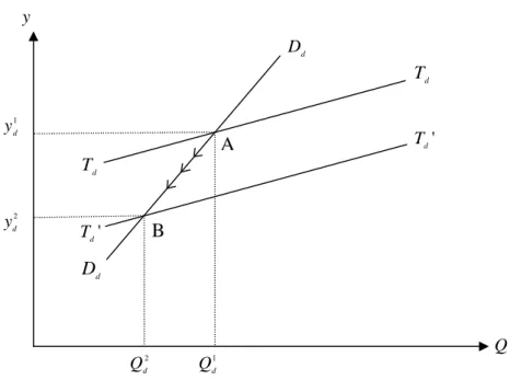
We explain the intuition behind Propositions 1(a) and 1(b) by using Figures 1 and 2, respectively. The reasoning behind Proposition 1(a) is as follows. Let us consider an increase in the property-tax rate on vacant land. Suppose that the initial equilibrium may be represented by point A, the intersection of lines D Dd d and T Td d in Figure 1, where a landowner develops
vacant land at the date y1d and at the density level Q .1d As indicated in equation (B4), when the
level of development density is fixed, an increase in this tax rate will be associated with less value from waiting, such that the landowner will develop earlier (as shown by the line T Td d that shifts downward to line T Td' d'). This, in turn, will induce the landowner to develop less densely, as indicated by equation (A4). The equilibrium point thus moves from point A along line D Dd d to point B, the intersection of the lines D Dd d and T Td' d'. As compared to the initial equilibrium
point A, at point B, the landowner develops vacant land at an earlier date yd2 (<y ), and chooses1d
a smaller density Qd2 (<Q ) as indicated by equations (B1) and (B2), respectively.1d The
statement in Proposition 1(a) will thus follow.
The reasoning behind Proposition 1(b) is as follows. As shown in Figure 2, suppose that the
initial equilibrium is at point A, where a landowner chooses a density equal to Q , and a date of1d
d D d T y Q 2 d y 1 d y B A 2 d Q d D ' d T d T 1 d Q ' d T
on the timing of development yd and the density of development Qd combines the two effects
stated below. First, when the level of development density is fixed, as this tax rate is increased, a landowner will develop later because the value of developed properties are decreased, as indicated by equation (B11) (This is shown by the line T Td d that shifts upward to the line T Td' d '). This, in turn, induces the landowner to increase the developed density because the landowner will be bold as long as the state at which he develops land is more favorable, as indicated by equation (A4). The equilibrium point thus moves from point A along line D Dd d to point B, where the
landowner chooses a density equal to Qd2 (>Q ), and a date of development equal to1d yd2 (>y ).1d
Second, as shown by equation (B13), when the timing of development is fixed, a landowner perceives that the net marginal benefit from developing land will be reduced such that the landowner will develop less densely (This is shown by the line D Dd d that shifts leftward to the line Dd'Dd'). This, in turn, will induce the landowner to develop earlier because waiting will then be less valuable when he develops less densely, as indicated in equation (A1). The equilibrium point thus moves from point B along line T Td' d' to point C. Summing these two effects may give rise to ambiguous results with regard to the choices of development timing and density. However, more precise calculations suggest that the landowner will develop later
(yd3 ) and at a larger density (y1d Qd3 ), as indicated by equations (B8) and (B9), respectively,Q1d as compared to the initial equilibrium point A.
11 ' d T y Q 2 d y 1 d y A d T ' d T 1 d Q 3 d Q ' d D d D ' d D Dd B C 3 d y d T 2 d Q Figure 2: An increase in a.
In Proposition 1(c), we also consider the case where uniform tax rates are imposed both before and after development. We then find that the impact of the property–tax rate on vacant land seems to dominate the choice of development density such that an increase in the tax rate will reduce development density, as indicated by equation (B15). However, the effect resulting from an increase in the tax rate on the choice of development timing is indefinite, as indicated by equation (B14).
We can compare our results with those of several studies that abstract from uncertainty and explore the relationship between taxation and land development. These studies include Anderson (1986), Turnbull (1988b) and Anderson (2005). All of them show that the effect of property taxation on choices regarding the timing and density of land development depends largely on the assumption as to whether the demanded density is increasing over time or not.8 In particular, they reach the same conclusion as our result stated in Proposition 1(a) for the case where the demanded density is increasing over time, which is analogous to our analysis indicating that land will be developed more densely at a better state, as shown by equation (A4). However, unlike our results in regard to Propositions 1(b) and 1(c), their results with regard to an increase in the property–tax rate after development or an increase of uniform property–tax rate are all indefinite even for this same case. This divergence arises because we impose specific functional forms for both the construction costs and the rent derived from developed property (as shown by equations (1) and (2), respectively), while their results are based on more general functional forms.
8
Our results stated in Proposition 1 are not fully in line with those of Capozza and Li (1994) who also employ a real–option model to investigate the timing and intensity decision of a landowner. Assuming that N 1, we can compare our results with theirs since they focus on a representative landowner. Capozza and Li assume that the scale developed by a landowner is of a Cobb-Douglas functional form in land and capital, which implies a cost functional form given by equation (1) in our framework. They also assume that the rent per unit of developed property is unrelated to the scale of developed property, which is analogous to imposing a0 and b1 in equation (2) in our framework. The key departure from our article is that they assume that the rent per unit of developed property follows an arithmetic Brownian motion, while we assume that it follows a geometric Brownian motion. With this departure, they find that an increase in the property–tax rate on undeveloped land accelerates development and reduces the capital intensity (and thus the development density), which is in line with our result stated in Proposition 1(a). However, they find that an increase in the property–tax rate on developed land delays that the expected development time and reduces the capital intensity. The former is in line with, while the latter is just the opposite of our results stated in Proposition 1(b). With uniform tax rates on property both before and after development, they find that an increase in the tax accelerates development and reduces capital intensity. The former is not in line, while the latter is in line with our results stated in Proposition 1(c).
This article can also investigate whether an increase in the tax rate before development and that after development ironically lead to a larger expected level of development density. This is stated in the following proposition.
Proposition 2: Suppose that h . (a) An increase in the tax rate before2( 2 1) / 2 1 development will result in a lower (higher) expected level of development density if
( ) 1/( )
h b a . (b) An increase in the tax rate after development will result in a higher
(lower) expected level of development density if h ( ) 1/ .
Proof: See Appendix C.
As shown in Proposition 2, when h 1/( b a), the long-run overbuilding problem will not occur when the regulator raises the tax rate before development. This premise is more likely to hold if (i) developers expect the costs of developing land to decline rapidly ( is relatively1 low), (ii) developers expect demand for developed property to grow rapidly ( is relatively high),2 or (iii) the net return derived from land development is less volatile ( is relatively low). This implies that the regulator is more likely to curb overbuilding under the following circumstances: development will eventually occur in the long–run regardless of whether this policy is implemented, including that future demand or supply conditions are favorable to developers, i.e., low or high1 , or that the environment in the real estate market as a whole is stable for2 developers, i.e., low . Under the same circumstances mentioned above, however, an increase
13
in the tax rate after development is more likely to lead to overbuilding in the long–run because the premise h 1/ is more likely to hold. We thus provide the conditions under which the regulator is able to avoid the long–run overbuilding problem when implementing taxation on property both before and after development.
2. The Centralized Economy
Consider the case of the centralized economy. A social planner will internalize the negative externality before choosing the development timing and density.9 We can thus impose
i
Nq andS Q on equations (1), (2), (4’a b 0 ), and (8), thus yielding the development cost function, the rent per unit of developed property, the value of property after development, and the value of vacant land if undeveloped forever perceived by the central planer, respectively, as given by:10 1 1 ( , ) ( ) , A Q C x Q x N (1’) 1 2 b a A R x Q , (2’) 2 2 2 ( , ) ( ) b a A x Q W x Q N , (4’’) 2 2 2 ( , ) ( ) B x W x N . (8’)
The social planner will choose an appropriate date and scale to maximize the expected present discounted value of the vacant land. This is defined as
1 2 2 1 2 ( , ) ( , ) ( , ), c B c V x x W x Z x x (7’) where ( ) 2 1 2 1 , ( ) ( , ) max { T t [ ( b a ) ( )( ) ]}. c t T T Q x Q Z x x E e Q d x T N N
(10’)In equation (10’), Z x xc( ,1 2) is the social value of a perpetual warrant to exchange the fixed Q units of developed properties for one unit of vacant land.
Define W x xc( ,1 2) as the intrinsic value of the warrant if exercised at time t , that is,
1 2 2 2 1 ( , ) max ( , ) ( , ) ( , ) c A B A Q W x x W x Q W x C x Q . (11’)9 We assume that the social planner internalizes the externality, but does not rectify market inefficiencies associated
with market power. Lee and Jou (2007) assume that the social planner rectifies market inefficiencies associated with both the negative externality and market power; however, they focus on the issue of the regulation of optimal development density.
10 Here and in what follows, we use the subscript “
c”to represent “centralized economy,”while subscript “A”and “B”represent “after”and “before”development in a centralized economy.
To maximize the intrinsic value at time t , the optimal scale, denoted by Q , must satisfy thec first-order condition for Q:
( 2, ) ( , )1
0 A A W x Q C x Q Q . (12’)Incorporating equation (11’) into (10’), we have
( )
1 2 1 2 ( , ) max T t ( ( ), ( )) c t c T Z x x E e W x T x T . (13’)Following similar arguments to those for the case of decentralized economy yields
1 1 1 2 1 2
1 2 1 2 1 2 2 1
( , ) ,
c c c
Z x x A x x A x x (15’)
where A1c and A2c are constants to be determined, and and1c are respectively equal to2c
2 2 1 2 1 1 1 2 2 2 ( ) ( ) 2( ) 1 1 ( ) , 2 2 c (16’) 2 2 1 2 1 1 2 2 2 2 ( ) ( ) 2( ) 1 1 ( ) . 2 2 c
Define yc (=x2c/x ) as the timing to develop vacant land and1c Qc as the density chosen by the social planner, respectively. Applying similar conditions as shown by equations (22)-(24) and (26), and imposing the constraint QQc on those conditions yields the counterparts of equations (25) and (27) as given by * 1 2 1 ( , ) (1 ) [ ] ( ) 0, ( ) b a c c c c c c y Q T y Q Q N N (25’) * 1 1 2 1 ( , ) 0. ( ) b a c c c c c c D y Q y Q N Q N (27’)
Solving equations (25’) and (27’) simultaneously yields
1 ( ) 2 ( 1) ( ) , ( ) b a c c y M b a N (28’) 1 (b a), c c Q M (29’) where 1 1 1 1 [1 (1 ) ] . c b a M (30’)
Equation (25’)implicitly definesthedependenceofyc on Q , while equation (27’c )implicitly defines the dependence of Qc on y .c We derive these two relationships in equations (D1)-(D7) in appendix D.
15
IV. Optimal Property Taxation
We will first assume that no property taxation is imposed, i.e. so as to comparea b 0 resource allocation under the decentralized economy with that under the centralized economy. Comparing equation (28) with equation (28’), and equation (29) with equation (29’) yields
d c
y y and Qd Qc if both N1 and . The more interesting case, however, isa b 0 where there is more than one landowner in which case we obtain the result stated below:
Proposition 3: When the real estate market is not monopolized, a landowner will develop property later, but more densely, than a central planner who fully internalizes the consumption-production externality.
Proof: Proposition 3 will follow given that Md Mc for N2, and .a b 0
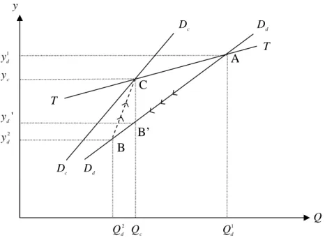
We use Figure 3 to explain the intuition behind Proposition 3. The same line TT depicts the dependence of the optimal date of development on the optimal density defined in both equation (25) given and equation (25’a b 0 ). This is because without any taxation, the existence of consumption-production externalities will be irrelevant to the choice of development timing. This line has a positive slope, thus indicating that, as property in the real estate market becomes more densely developed, both a landowner and the central planner will be less eager to develop property since the rent per unit of developed land will then be lower, and thus waiting will be more valuable. On the other hand, the lines D Dd d and D Dc c depict the dependence of the optimal density on the optimal date of development defined in equation (27) given anda b 0 equation (27’), respectively. Both lines have a positive slope, which indicates that, at a better state, both a landowner and the central planner will develop property more densely.
Given that N2 and , linea b 0 D Dc c will lie to the left of line D D .d d This indicates that, given the same timing of development, a central planner who internalizes the externality will develop property less densely than a landowner who ignores the same externality. The central planner will thus develop earlier than the landowner, as indicated by the positive slope of the line TT. This is shown by Point C that denotes the equilibrium for a central planner,
which is where the lines TT and D Dc c intersect, for which the optimal density is Qc and the
optimal date of development is y .c By contrast, Point A denotes the equilibrium for a landowner,
which is where the lines TT and D Dd d intersect, and where the optimal density is Q1d and the
c D Dd T y Q c y A B 1 d Q c D Dd T c Q 1 d y 2 d Q 2 d y C B’ ' d y
Figure 3: Difference between the centralized and the decentralized economy.
Proposition 3 indicates that the market outcome is inefficient for N2. Therefore, a social planner, who fully perceives the negative externality, can design a property taxation policy to correct this outcome. As mentioned before, our model presents a hierarchical game. At the lower level, a landowner competes with the other landowners, and chooses both a date of
development equal to yd and a density level equal to Qd in a Cournot-Nash environment. At
the upper level, the regulator acts as a leader and the landowner acts as a follower. The regulator anticipates that both the timing and density chosen by the landowner will be above the socially
optimal level, yc and Q , respectively.c Consequently, the regulator needs to impose property
taxation both before and after development so as to align the timing and density chosen by the
landowner with those chosen by the central planner. Equating yd in equation (28) with yc in
equation (28’) and equating Qd in equation (29) with Qc in equation (29’) yields the optimal
tax rates after and before development, and*a , respectively, as given by*b
* 2 1 1 ( )(1 )( 1) 0, a N b a (31) * * 1 1 * 1 1 2 ( ) ( ) 1 ( 1 ) 1 [1 ][1 (1 ) ] 1 (1 ) . ( ) a b c d b b a N b a N (32)
17
The design of taxation before and after development can be explained by using Figure 3. As mentioned before, points A and C represent the equilibrium points for the decentralized and the centralized economy, respectively. As indicated by Proposition 1(a), when the regulator imposes
a tax rate on property before development, a landowner will be induced to move downward*b along D Dd d until point B, where he develops property at a date equal to yd2 and a density equal
to Q .d2 As indicated by Proposition 1(b), when the regulator further imposes a tax rate on*a property after development, the landowner will be induced to move upward from point B to point C, the equilibrium point for the centralized economy. Note that if the central planner only imposes taxation before development, a landowner may be induced to develop on the same scale as the centralized economy, but earlier than will be socially optimal. For example, in Figure 3, a
landowner will develop property atpointB’,wherethe development density is equal to Q , whilec the development timing is equal to yd3 (yc).
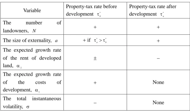
Table 1 shows how changes in several exogenous variables affect optimal taxation before and after development, which we state in the following proposition:
Proposition 4: (a) The regulator should increase property taxation both before () and after (*b )*a development if there are more landowners in the real estate market (N is larger). (b) The regulator should increase property taxation after development, but may increase, reduce, or leave unchanged property taxation before development if (i) the negative externality becomes more significant (a is larger), or (ii) demand for developed property is expected to grow more slowly ( is smaller). (c) The regulator should raise property taxation before development, while2 leaving taxation after development unchanged if (i) the development costs are expected to grow more rapidly ( is larger), and (ii) uncertainty is reduced (1 is lower).
Proof: See Appendix E.
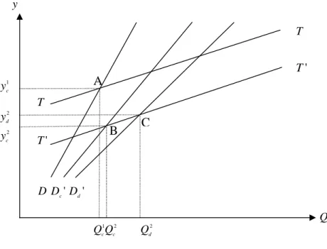
We can use Figure 4 to explain the reason for Proposition 4(a). Suppose that the initial equilibrium is depicted by point A, which is the intersection of lines TT and DD, both of which are the common lines of the centralized economy and the decentralized economy with appropriate property taxation to correct market inefficiencies. When the scale of development is fixed, an increase in the number of landowners will reduce the expected development time by the same magnitude for both the centralized and the decentralized economy, as indicated by equation (E11)
' T y Q 1 c y 2 d y A 2 d Q T 1 c Q 2 c Q B C 2 c y T ' T D Dc'Dd'
(This is shown by a downward shift from line TT to T T' '). Furthermore, when the choice of development timing is fixed, an increase in the number of landowners will induce a landowner to increase the development density by a magnitude that outweighs the increase in the development density for a central planner because the landowner ignores the negative externality. This is indicated by equations (E12) and (E13), and is shown by an outward shift from line DD to lines
' '
d d
D D and D Dc' c' for the decentralized and the centralized economy, respectively. As indicated by Proposition 1, the regulator needs to raise taxation both before and after development because the new equilibrium for the centralized economy, point B, is on the south-western side of the new equilibrium for the decentralized economy, point C. The other results stated in Proposition 3 can also be derived using similar arguments.
Figure 4: An increase in N.
The results of Proposition 3 (or Table 1) accord well with intuition. First, as the negative externality becomes more severe either by itself (a is larger) or results from an increase in the number of landowners (N is larger), the regulator should raise taxation both before and after development in response.11 Second, as future demand for developed property is expected to grow more slowly ( is lower), a developer will be induced to develop property earlier, but on a2 smaller scale as compared to a social planner. The regulator thus needs to raise taxation after development, as indicated by Proposition 1(b) (The impact on taxation before development, however, is indefinite). Third, as the costs of development are expected to grow more rapidly, the optimal condition for the choice of density of development for both a landowner (equation (25)) and a social planner (equation (25’)) will not be affected. Consequently, the regulator only needs
11 Note that an increase in the magnitude of the externality has a positive impact on taxation before development, * b , only in the region where * *
b a
19
to raise taxation before development so as to encourage a landowner to develop earlier, but on a smaller scale, while leaving taxation after development unchanged. Finally, the total instantaneous volatility () will be greater as r12 is lower, i.e., as x t1( ) and x t2( ) move in the opposite directions. That is, uncertainty will be greater if more (less) advantageous supply conditions are associated with more (less) prospective demand conditions in the real estate market. The impact of greater uncertainty resembles that of a lower expected growth rate in relation to the development costs, and thus the regulator only needs to reduce taxation before development.
We assume that developed property exhibits a negative externality on urban residents, while vacant land does not exhibit any externality. To correct this externality, however, it is uncertain
whether the rate of property taxation after development should be higher than that before*a development . We, however, can compare the order of*b and*a around the region where*b
* *
a b
, as stated in the Proposition below:
Table 1: Comparative-Statics Results
Variable Property-tax rate before development *
b
Property-tax rate after development *
a
The number of
landowners, N
The size of externality, a if * * b a
The expected growth rate of the rent of developed land, 2
The expected growth rate
of the costs of
development, 1
None
The total instantaneous
volatility, None
Proposition 5: Starting from a coincidence of and*a ,*b should be higher than*a if (a)*b the number of landowners increases; (b) the costs of development are expected to grow less rapidly, or the total instantaneous volatility is greater.
Proposition 5(a) follows because as the number of landowners increases, both and*a *b will then be raised (as stated in Proposition 4(a)), but the latter will be raised by a smaller magnitudes than the former as indicated by equation (F1). Proposition 5(b) follows because as the costs of development are expected to grow less rapidly, or the total instantaneous volatility is
greater (as stated in Proposition 4(c)), will then be lower, while*b will remain unchanged.*a
VI. Conclusion
This article investigates the design of property taxation both before and after development in a real options framework where a fixed number of landowners irreversibly develop property in an uncertain environment. We assume that densely developed properties reduce open space, and thereby harms urban residents. However, landowners will ignore this negative externality, and will thus develop properties more densely than is socially optimal. The regulator can correct this tendency by imposing taxation on property both before and after development. We then find that the tax on the former should be increased if the real estate market consists more landowners, the costs of development are expected to grow more rapidly, and uncertainty is less significant. In addition, taxation on the latter should be increased if the real estate market consists more landowners, the externality is more significant, or if demand for property after development is expected to grow less rapidly. Future studies may empirically test these theoretical predictions.
This article can be extended to investigate the issue discussed in Henry George’s seminal book Progress and Poverty (1897), i.e., taxation on vacant land should be higher than taxation on land development. Brueckner (1986) has investigated how a shift to a graded tax system (where the tax rate is lowered and the land tax rate it raised) affects the level of development, the value of land and the price of housing in the long-run. Anderson (1993b) has extended the Brueckner’s analysis by employing a perfect foresight model. His focus is how this shift affects choices regarding the timing and density of development. If we replace taxation on property after development by taxation on development, we not only can investigate the issue discussed in Anderson (1993b), but can also investigate whether there exists a tradeoff between land value taxation and land development taxation when these two instruments are employed to correct the externality associated with land development.
21
Appendix A:
Totally differentiating equation (25) with respect to Q , and using equations (28) -(30) yieldsd
12 11 0, d d y Q (A1) where * 11 ( , ) 1 ( ) 0, d d d d d d T y Q Q y y N (A2) * 12 1 2 ( , ) 1 ( ) (1 ) ( ) 0. ( ) ( ) d d d d d d d a d T y Q y b a M Q N Q b a (A3)
Totally differentiating equation (27) with respect to y , and using equations (28)-(30) yieldsd
21 22 0, d d Q y (A4) where * 1 2 22 ( , ) ( ) 0, d d d d d D y Q b a N Q Q (A5) * 1 21 2 ( , ) ( 1 ) 0. ( ) b a d d d d d a D y Q N b a Q y N (A6)
The Jacobian condition also requires that
11 22 12 21 0.
(A7)
We depict the impact of Qd on yd in equation (A1), and that of yd on Qd in equation (A4) by line T Td d and line D Dd d in Figure 1, respectively. Equation (A7) requires that the slope of
d d
D D be steeper than that of T T , and we find that this requirement is satisfied.d d
Appendix B:
Totally differentiating both yd in equation (25) and Qd in equation (27) with respect to
b yields ( 1) 0, ( ) d d d d d d b b d b d b dy y y Q y M d Q b a M (B1) ( ) ( ) (0)
0, ( ) d d d d d d b b d b d b dQ Q Q y Q M d y b a M (B2) (0) ( ) ( ) where 13 11 0, d b y (B3) since * 1 13 2 2 1 2 2 2 1 ( ) 1 1 (1 ) [ ] 0, ( ) ( ) ( ) b a d d d d d b d b a b d b T y y Q d N d N (B4) where 1 1 1 ( ) 0, ( ) d d d b b d d d d because ,d( 1d) b 1 and 2 1 1 2 1 ( ) / (2 1) ( ) 0 2 d d d , 23 22 0, d b Q (B5) because 23 d( ) 0, b D (B6) and 2 1 1 1 1 1 1 1 [( ) (1 ( 1 )(1 ) ) ] 0 d d b b d M M N b a B N , where 1 ( ( 1 ))( 2( 1 1) (2 1 1)) 1 0 2 d d N b a B N N . (B7)
Totally differentiating yd and Qd with respect to yieldsa
2 0, ( )( ) d d d d d a a d a a dy y y Q y d Q b a (B8) ( ) ( ) ( ) 2 0, ( )( ) d d d d d a a d a a dQ Q Q y Q d y b a (B9) ( ) ( ) ( ) where 14 11 0, d a y (B10) since * 14 2 1 2 ( , ) 1 (1 ) 0, ( ) b a d d d d d a d a T y Q y Q N (B11)
23 and 24 22 0, d a Q (B12) since * 1 24 2 2 ( , ) ( 1 ) 0. ( ) b a d d d d d a a D y Q N b a y Q N (B13)
Let . Substituting this equality intoa b yd and Q , and then differentiating withd respect to yields 1 2 ( 1) 0, ( )( ) ( ) d d d d y y B y M b a b a (B14) 1 0, ( ) d d d Q B Q M b a (B15)
where B is defined in equation (B7).1
Appendix C: Define 2 1 2 2( ) 1 h
. Following Riddiough (1997), given any y , the probabilityyd
that y eventually hits yd in the long run is given by
( ) 1 , if 0, ( ) , if 0. d h d F y h y h y (C1)
The long-run expected level of density is given by multiplying Fd( )y by Q , thus yieldingd
1 ( ) ( ) , if 0, , if 0, d d d h b a h h d d F y Q Q h A Q y h (C2) where 2 2 (1 )( ) . ( 1 ) d u A N b a N
Differentiating Fd( )y Qd with respect to yieldsb
( ( ) ) 0, if 0, d d d b b d F y Q dQ h d d (C3) (1 ( )) d( ) d 0, b dQ h b a F y d if both h0 and h( b a) 1, where d 0 b dQ
d by equation (B1). The statement in Proposition 2(a) will follow since
( ( ) ) 0, if 0, d d d a a d F y Q dQ h d d (C4) 2 ( ) (1 ) 0, ( )( ) d d a F y Q h b a if h 1/ .
This completes the proof.
Appendix D:
Totally differentiating equation (25’) with respect to Qc and using equations (28’)-(30’) yields 12 11 0, c c y Q (D1) where * 11 1 2 ( , ) 1 ( ) (1 ) 0, ( ) c c c c c c T y Q M y N (D2) * 12 1 2 ( , ) 1 ( ) (1 ) ( ) 0. ( ) ( ) c c c c c c c c T y Q y b a M Q N Q b a (D3)
Totally differentiating equation (27’) with respect to y , and using equations (28’c )-(30’) yields
21 22 0, c c Q y (D4) where * 2 22 ( , ) ( ) 0, c c c c c D y Q b a N Q Q (D5) * 1 21 2 ( , ) ( ) 0. ( ) b a c c c c c D y Q b a Q y N (D6)
The Jacobian condition also requires that
11 22 12 21 0.
(D7)
We depict the impact of Qc on yc in equation (D1), and that of yc on Qc in equation (D4) by line TT and line D Dc c in Figure 3, respectively. Equation (D7) requires that the slope of line D Dc c be steeper than that of line TT in Figure 3, and we find that this condition is satisfied.
25
Define respectively the left-hand and right-hand sides of equation (32) as F( and*a, *b; )
* *
( a, b, )
G , where N , a , ,2 , or1 . Totally differentiating in equation (31) and*a both sides of equation (32) with respect to N yields
* 2 2 1 1 ( )[ 1] 0, ( ) a d dN N b a (E1) * * 1 * ( ) ( ) ( ) 0, b a a d F G dN N N (E2) since * * ( ) ( ) 0 b b G F and G( ) / N 0.
Totally differentiating and both sides of equation (32) with respect to a yields*a
* 2 2 ( ) 1 (1 ) 0, ( ) a a b a N (E3) * * 1 * ( ) ( ) ( ) ( ) 0, b a a F F G a a a a (E4) since F( ) / a 0 and G( ) / a 0.
Totally differentiating and both sides of equation (32) with respect to*a yields2
* 2 2 1 1 ( 1) 0, ( ) a b a N (E5) * * 1 * 2 2 2 2 ( ) ( ) ( ) ( ) 0, b a a F F G (E6) since andF( ) / 2 0 .G( ) / 2 0
Totally differentiating and both sides of equation (32) with respect to*a yields1
* 1 0, a (E7)