應用共同成本函數探討歐洲16國銀行業的生產效率

國立交通大學

國立交通大學

國立交通大學

國立交通大學

財務金融所

碩士論文

應用共同成本函數探討歐洲 16 國銀行業的生產效率

Estimation of Technical Efficiency and Technology Gaps for Banks

in 16 European Countries Using a Meta-frontier Cost Function

研 究 生：邱柏豪

指導教授：黃台心 博士

鍾惠民 博士

應用共同成本函數探討歐洲 16 國銀行業的生產效率

Estimation of Technical Efficiency and Technology Gaps for Banks

in 16 European Countries Using a Meta-frontier Cost Function

研 究 生：邱柏豪 Student：Po-Hao Chiu

指導教授：黃台心 博士 Advisors：Dr. Tai-Hsin Huang

鍾惠民 博士 Dr. Huimin Chung

國立交通大學

財務金融所

碩士論文

A Thesis

Submitted to Graduate Institute of Finance

National Chiao Tung University

in partial Fulfillment of the Requirements

for the Degree of

Master of Science

in

Finance

June 2006

Hsinchu, Taiwan, Republic of China

應用共同成本函數探討歐洲 16 國銀行業的生產效率

研 究 生：邱柏豪 指導教授：黃台心 博士

鍾惠民 博士

國立交通大學

財務金融研究所

2006 年 6 月

摘要

本篇論文主要欲探討歐洲 16 個國家商業銀行的成本效率，但是，在過去的 研究中並無法針對不同生產技術下的銀行直接做效率的比較，所以我們便利用了 Battese、Rao 和 O’donnell (2004)所提出的共同函數模型來當我們研究的基 礎，其模型主要建立在不同技術下的效率研究。而在實證的資料中，我們發現了 歐洲 16 國中彼此的生產技術的確存在顯著的差異，並且各銀行的技術亦也有大 幅的波動。 關鍵字: 技術效率; 技術缺口; 隨機邊界成本函數; 共同邊界成本函數; 線性 規劃; 二次規劃

Estimation of Technical Efficiency and Technology Gaps for Banks

in 16 European Countries Using a Meta-frontier Cost Function

Student：Po-Hao Chiu Advisors：Dr. Tai-Hsin Huang

Dr. Huimin Chung

Graduate Institute of Finance

National Chiao Tung University

June 2006

ABSTRACT

In this thesis, we will investigate the cost efficiency of commercial banks across 16 European countries. It is important to note that the technical efficiency of a bank operating under a type of technology is not directly comparable with that of other bank operating under a different type of technology. Therefire, we adopt a meta-frontier production function, proposed by Battese, Rao, and O’donnell (2004), which allows for the calculation of technical efficiencies for banks operating under different technologies.

Keywords: Technical Efficiency; Technology Gaps; Stochastic frontier cost function; Meta-frontier Cost Function; Linear programming; Quadratic programming

致謝

致謝

致謝

致謝

一眨眼

，兩年的時光便以消逝，而待在交大財金所的日子也到了尾聲，在 此求學的過程讓我對生命有了新的體悟，甚至這裡的環境、教學、師長、同學和 學弟妹都在我生命中亦佔有了不可抹滅的影響，我亦很高興能走此一遭。這次論 文的完成，首先我要感謝黃台心老師，在這段時間，每當我在理論、資料或是程 式遇到障礙時，我總是不斷的麻煩老師，但老師總是不厭其煩的為我解惑，對此 我深深感激，再來，我要謝謝鍾惠民老師，總是不斷關心我論文的進度，亦給了 我不少在研究上的值得索思想法，還有我要謝謝此次論文的口試委員：傅祖壇老 師和陳忠榮老師，給了我不少值得研究的方向，讓我的論文更趨完善。 而在論文撰寫的過程中，我還要感謝我許多的好朋友：感謝俊宇總是在我 失意時拉我一把；感謝阿達能跟我在這枯燥的論文過程一起努力，一起持續運 動，可堪稱是個好夥伴；感謝家農哥所提供的漫畫，能讓我偶爾解解悶；感謝揮 哥在我程式遇到瓶頸時給我正確的方向；感謝忠穎可以在財務理論跟我一組，真 是分擔了不少壓力；感謝惠華和瑞娟能在默默接受我這顆課的話語，雖然我都笑 你們胖，但真的是要激勵你們減肥；此外也要感謝儀貞，在研究所的日子能一起 努力；再來要感謝尉如學弟總是辛勞的幫我整理資料；最後就是要感謝我們電影 團所有的團員，在這段日子分享了不少電影。 很謝謝我的爸爸、媽媽和姊姊們，唯有家人的支持，我才能有今日的成果， 謝謝你們的關愛和支柱。 邱柏豪 謹誌於 交通大學財務金融所 民國九十五年六月

Content

1. Introduction... - 2 -

2. Literature Review ... - 3 -

2.1 Efficiency studies on European Banking ...- 3 -

2.2 Meta-frontier model...- 5 -

3. Methodology ... - 7 -

3.1 Stochastic Meta-frontier Cost Function...- 8 -

3.2 Technology Gap and Efficiency Levels ...- 10 -

3.3 Formula of the Scale and Scope Economies ... - 11 -

3.4 Estimation Procedure ...- 12 -

4. Data Source and Variable Definition ... - 14 -

5. Empirical Results... - 16 -

5.1 Parameter Estimates...- 16 -

5.2 Cost Efficiency and Technology Gap Ratio ...- 29 -

5.3 Scale and Scope Economies...- 34 -

6. Conclusion ... - 35 -

1. Introduction

Following the disasters of the First World War and the Second World War, the incentive for peaceful unification through collaboration and equality of member states greatly increased. These increasing impulses of achieving the formation of the EU were come from the thirst for rebuilding Europe and expectation to get rid of the possibility of another such terrible war arising again. As a result, this momentum led to the establishment of the European Coal and Steel Community by West Germany, France, Italy and Benelux countries. Then, the European Union or EU was founded in 1992 by Treaty of European Union (the Maastricht Treaty).1

The Treaty of Maastricht in 1992 also sets up the European Economic and Monetary Union (EMU).2 In economics, a monetary union is an agreement that member countries utilize a common currency among them. The EMU not only creates a single currency, the Euro, but also sets a lot of economic convergence principles, including exchange rate, inflation rate, public finance and interest rates stability. All member states of the European Union have a hand in the EMU. In the recent years, through the endeavor of the EMU, many member states have adopted the new criteria to regulate their financial markets in order to lower barriers to competition among financial institutions. For example, a bank will only be regulated by its home country even though it plans to open a new branch in any other country. All these changes help intensify the degree of competition in European financial markets. Lower production cost and higher economic efficiency may result.

As the financial markets become more and more competitive and integrated, each country’s banking structure and oncoming competitive viability are greatly

1

The Maastricht Treaty (formally, the Treaty on European Union) was signed on 7 February 1992 in Maastricht between the members of the European Community and entered into force on 1 November 1993, under the Delors Commission.

2

determined by the current differences in managerial performance. Therefore, it is important to understand what are the differences or similarities in the production efficiency of banks among countries. In this thesis, we will investigate the cost efficiency of commercial banks across 16 European countries. It is important to note that the technical efficiency of a bank operating under a type of technology is not directly comparable with that of other bank operating under a different type of technology. However, the conventional studies on the comparisons of production efficiency are unable to distinguish the possibilities of various technologies employed by sample firms. Therefore, we adopt a meta-frontier production function, proposed by Battese, Rao, and O’donnell (2004), which allows for the calculation of technical efficiencies for banks operating under different technologies.

The thesis is organized as follows. Chapter 2 is the literature review. Chapter 3 develops a meta-frontier cost function under a one-stage process. In chapter 4, the data and the definitions of input and output variables are described, while in chapter 5 technical efficiencies for banks and technology gaps for countries are empirically evaluated in a context of meta-frontier cost methodology. The last chapter concludes the thesis.

2. Literature Review

2.1 Efficiency studies on European Banking

In the recent years the structure of European banking has been changing rapidly. The implementation of the Single Banking Market during the nineties lowered barriers to competition among European banks and helped them to expand branches abroad within the members of European Union more easily. The financial markets have become more and more competitive and integrated. Therefore, it is important to understand the sources of the banks’ efficiency differences among countries.

There are three main approaches to measure technical efficiency of individual banks, the stochastic frontier approach (SFA), the distribution-free approach (DFA) and the data envelopment analysis (DEA). The SFA, developed by Aigner et al. (1977) and applied to the bank industry by Ferrier and Lovell (1990), needs to specify a particular function form, and its error term is composed of two elements. One of them represents the production inefficiency, which is usually assumed to be disturbed as a truncated or half-normal distribution, and the other follows a symmetric normal distribution. The former error term is nonnegative by construction and is used to reflect production inefficiency. Altunbas et al. (2001) applied the flexible Fourier functional form to the stochastic cost frontier function and found that banks of all sizes could save their cost by reducing managerial and other inefficiencies. Vennet (2002) analyzed the cost and profit efficiency of European financial conglomerates and universal banks and found that the trend toward de-specialization may lead to a more efficient banking system. Bonin et al. (2005) and Fries et al. (2005) applied the SFA model to investigate the bank efficiency in transition countries. They found that private banks are more efficient than government-owned banks and, foreign-owned banks are more efficient than other types of banks.

The DFA, proposed Berger (1993), assumes that the inefficiency of each bank is firm specific and constant over time in the context of panel data. Then, each firm’s production inefficiency is measured as the difference between its fixed effect estimate and that of the best practice bank. The distribution of inefficiencies in the DFA model can follow almost any form, as long as they are non-negative. Maudos et al. (2002) employed the DFA approach to make cross-country comparison and uncovered that there is a wide range of variation in efficiency levels in the banking system of the European Union, especially the variation in profit efficiency being greater than in cost efficiency.

Finally, DEA imposes less structure on the efficiency frontier than does the parametric approach, because it does not need to specify any functional form for the frontier. However, it is frequently criticized as ignoring the error term. Consequently, the estimates of inefficiency using DEA are unable to distinguish the stochastic component from the efficiency measure. Berg et al. (1993, 1995) used DEA to capture the differences or similarities in the efficiency of banks among the Nordic countries. Lozano-Vivas et al. (2001, 2002) and Ana et al. (2002) improved the conventional DEA model by incorporating environmental factors into their models and found that country-specific environmental conditions exert a strong influence on the behavior of banks.

In making comparisons of banking efficiency across countries, we need to estimate a common frontier for all banks in these countries under consideration. It is important to simultaneously consider country-specific environmental conditions, which influence the level of efficiency for all banks. If we simply pool all banks across countries without regard to the impact of the environmental differences, we are implicitly assuming that efficiency differences across countries are entirely ascribable to managerial ability of banks. Biased estimates may result. Therefore, we adopt a meta-cost frontier function, proposed by Battese et al. (2004), to estimate bank efficiency across countries. This function allows for the calculation of technical efficiencies for banks operating under different technologies.

2.2 Meta-frontier model

Hayami (1969) first proposed the meta-frontier production function to examine the causes of agricultural productivity differences among the developed and less developed countries, followed by Hayami and Ruttan (1970, 1971). Hayami and Ruttan (1970, 1971) made a crucial assumption that the technological possibilities

available to all agricultural producers in different countries under consideration can be characterized by the same production function, namely the meta-production function. This concept is theoretically attractive, because it is based on the simple hypothesis that all producers in different countries have potential access to the same technology, and it allows for the comparisons of production efficiencies among producers operating under different technologies. However, one may notice that the meta-production function does not imply that all producers operate on a universal production function. The meta-production function, proposed by Ruttan et al. (1978), is an envelope curve of production points of the most efficient countries. Each country may choose to operate on different part of the production possibility curve, depending on its resource endowments, adoption and diffusion of technology, and economic environments.

Following the seminal work of Hayami and Ruttan (1970, 1971), Lau and Yotopoulos (1989) employed the meta-production function approach to compare agricultural productivity across countries. They addressed some econometric advantages of applying the meta-production function. This approach is particularly able to pool data from different countries to estimate a common production function, thus increasing the range of variation of the independent variables and the number of observations. Moreover, it reduces the possibility of multicollinearity among inputs, as various inputs are usually changing together. Consequently, more precise and reliable parameters estimates may be obtained. Several limitations inherent to this approach are worth mentioning. The non-comparability of data, the differences in the basic economic environments and the specification of an appropriate production function pose some difficulties.

Sharma and Leung (2000) and Gunaratne and Leung (2001) further adopted a stochastic meta-frontier model. The setting is exactly the same as the standard

stochastic frontier approach (SFA), originally proposed by Aigner, Lovell, and Schmidt (1977). Sharma and Leung (2000) studied the technical efficiency of aquaculture farms in several South-Asian countries, using the model developed by Battese and Coelli (1995) under the framework of the stochastic meta-frontier function, where the effects of various firm-specific variables on technical efficiency were simultaneously investigated.

Battese and Rao (2002) attempted to compare the technical efficiencies of firms in different groups that may not have the same technology on the basis of the stochastic meta-frontier production function. They assumed that there are two different data-generation mechanisms for the data, one with respect to the stochastic frontier that is estimated using data belonging to that group, and the other with respect to the meta-frontier model that is estimated using entire sample data. The estimation of the technology gap helps us identify the ability of the firms in one group to compete with other firms from different groups within an industry. Following Battese and Rao (2002), Battese, Rao, and O’donnell (2004) modified the above model by assuming that data-generation processes are only applied for the frontier models for the firms in the different groups. Meanwhile, the meta-frontier function is an overarching function of a given mathematical form that envelopes the deterministic components of the stochastic frontier production functions for the firms that operate under different technologies involved.

3. Methodology

In this chapter, we present the methodology to be used to estimate cost efficiency, technology gap, scale economies, and scope economies. As discussed by Berger and Mester (1997), the adoption of the economic efficiency concepts will

provide further insights into the problem of the economic optimization.3 The cost efficiency is undoubtedly an appropriate approach since the European financial markets have been more competitive and highly integrated. The main idea comes from Battese et al. (2004) while generalized to a cost frontier setting.

3.1 Stochastic Meta-frontier Cost Function

Cost efficiency is gauged by the extent to which a bank’s actual cost deviates from the efficient cost frontier. We first introduce the stochastic cost frontiers of the banking industry for each country. Suppose that there are R different countries under consideration, and that each country k has N banks that face input prices and _k seek to minimize the cost which they incur in producing the outputs. The stochastic cost frontier model for each bank w of country k at time t can be given as

,

,

,

2

,

1

;

,

,

2

,

1

;

,

,

2

,

1

,

)

,

(

( ) ( ) ) ( ) ( ) (

R

k

T

t

N

w

e

X

f

C

k U V k k wt k wt k wt k wt

K

K

K

₌

₌

=

=

ϕ

+ (1) where C_wt(k) is the total expenditure, X_wt(k) is a vector of outputs and input prices,

) ( k

ϕ is the unknown technology parameter vector to be estimated. V_wt(k) and U_wt(k) are identically and independently distributed random variables. The former is assumed to be distributed as N( 0 , σ2 ν (k) ), capturing the statistical noise, and the

latter is assumed to be a truncated normal distribution, a positive disturbance capturing technical inefficiency, to be specified shortly. For expository convenience, equation (1) is further formulated as

) ( ) ( ) ( ) ( ) ( k wt k wt k k wt V U X k wt e C = ϕ + + (2) The model, as proposed by Battese et al. (2004), assumes that there is only one

3

data-generation process for the banks operating under a given technology for each country. The data is individually generated from the frontier models in the different countries. In general, the meta-frontier is assumed to have the same functional form as the stochastic frontiers in the different countries. Thus, the meta-frontier cost function for all banks is given by

T t N N w e X f C R k k X wt wt wt ,..., 2 , 1 ; ,..., 2 , 1 , *) , ( 1 * * = = = ≡ =

∑

= ϕ

ϕ

(3)

where C_wt* is the minimum expenditure incurred by the bank w in year t; ϕ* is the corresponding parameter vector associated with the meta-frontier cost function

such that ) ( * _{wt k} wt X X ϕ ≤ ϕ (4) The meta-frontier is defined as a deterministic parametric function such that its values

must be less than or equal to the deterministic components of the stochastic cost

frontier of the different countries involved. The inequality constraint of equation (4) is

held for all countries and time periods. The meta-frontier is considered to be an

envelope of the individual stochastic frontiers of the different countries. Figure 1

provides an illustration of how the meta-frontier envelopes the stochastic frontiers of

the different countries. We will estimate the stochastic cost frontiers for each country,

denoted by frontier1, frontier2 and frontier3 in the figure. Then, a meta-frontier is

estimated as an envelope curve which surrounds the three stochastic frontiers from

3.2 Technology Gap and Efficiency Levels

Cost efficiency is determined by how close a bank’s cost lie to the overall cost

frontier, namely the meta-frontier. Therefore, the measure of cost efficiency (CE*) for

bank w in year t is formulated by the ratio of the minimum cost to observed cost, adjusted by the corresponding random error,

) ( * * ) ( ) ( k wt V X k wt C e CE k wt wt + = ϕ (5)

Substituting (2) into (5), we obtain

) ( ) ( ) ( ) ( ) ( ) ( * * * ) ( _{wt k} wt k wt k wt k wt k wt k wt wt X X U U V X V X k wt e e e e e CE _ϕ ϕ ϕ ϕ × = = − + + + (6)

where the first term on the right-hand side of equation (6) is the conventional

technical efficiency (CE) relative to the stochastic frontier of country k ,

) ( ) ( ) ( ) ( ) ( ) ( ) ( k wt k wt k wt k wt k wt k wt U U V X V X k wt e e e CE _{+ +} − + = = _ϕ ϕ (7)

construction. The second term on the right-hand side of equation (6) is the technology

gap ratio (TGR), i.e.

) ( * ) ( _{wt k} wt X X k wt e e TGR _ϕ ϕ = (8) The TGR mainly evaluates the degree of technology gap for country k whose

currently available technology adopted by its banks lags behind the technology

available for all countries. We measure the TGR using the ratio of the potential cost

that is defined by the meta-frontier function to the cost for the frontier function for

country k given the observed outputs and input prices. It has a value between zero

and one because of equation (4).

The cost efficiency measure of equation (5) can be expressed as

) ( ) ( * ) (k wt k wtk wt CE TGR CE = × (9) CE* also lies between zero and one because CE and TGR are both between zero and

one.

3.3 Formula of the Scale and Scope Economies

In the context of multiple outputs, a formal measure of scale economies is

referred to as ray scale economies (RSE), developed by Baumol et al. (1982) and

applied to banking by Berger et al. (1987). It is defined as

∑

_∂∂ = i yi f RSE ln ln (10)

where y is the ith output produced by a bank and f is its cost function. An _i estimate of RSE less than, equal to, or greater than 1 indicates, respectively, scale

economies, constant returns to scale, or scale diseconomies.

Economies of scope exists when total cost of a firm simultaneously producing

more than one output are lower than the sum of the costs of firms producing each

Mester (1996), the estimate of scope economies is defined as

[

]

) , ( ) , ( ) , ( ) , ( 2 1 2 1 2 2 1 2 1 1 y y f y y f y y y f y y y f SC m m m m _{+ − −} − = (11)

where y_im is 10% of the minimum value of y_i in the sample. The purpose of using

m i

y , instead of zero in the equation, avoids taking the logarithms of zero in the

translog function. An estimate of SC greater than, or less than zero indicates,

respectively, scope economies or scope diseconomies.

3.4 Estimation Procedure

Now that we have introduced the meta-frontier model, the next step is to

estimate the technology parameters of the cost function. The estimation procedure is

divided into three steps:

1. Obtain the maximum likelihood estimates,ϕˆ_(k), of ϕ_(k) in the stochastic cost frontier for country k . The stochastic frontier model proposed by Battese and

Coelli (1992), which allows for time-varying technical efficiency, will be

adopted.

2. Obtain the estimate of ϕ* in the meta-frontier. Battese et al. (2004) pointed out that there are two approaches to find out the best envelop curve. Detailed see

below.

3. According to equations (6)-(11), calculate the cost efficiency, the technology gap,

scale economies ,and scope economies, using ϕˆ_(k) and

ϕ

ˆ* obtained by Step 1

and 2.

We now return to the estimation procedure on the meta-frontier. There are two

alternative approaches can be applied to identify the best meta-frontier. One is based

frontiers, and the other is based on the sum of squares of the same deviations.

I. Minimum sum of absolute deviations

* ˆ

ϕ

is estimated by solving the optimization problem:

∑∑

= = − ≡ T t N w wt k wt f X X f L 1 1 ) ( ) ln ( , *) ˆ , ( ln * min ϕ ϕ (12) s.t.ln f(X_wt,ϕ*)≤ln f(X_wt,ϕˆ_(k)) (13) It will be clear from equation (12) and (13) that the estimated meta-frontier

minimizes the sum of absolute logarithms of f(X_wt,ϕˆ_(k))/ f(X_wt,ϕ*), which represents the reciprocal of the radial distance between the meta-frontier and the

frontier of country k . The weights of the deviations for all banks in the

sample are the same. One may notice that all the deviations are positive because

of equation (13). Therefore, all the absolute deviations are exactly equal to the

differences. Using equations (2) and (3), we can simplify the above optimization

problem to the linear programming (LP) problem:

∑∑

(

)

= = − ≡ T t N w wt k wt X X L 1 1 ) ( * ˆ * min ϕ ϕ (14) s.t.X_wtϕ ≤* X_wtϕˆ_(k) (15) II. Minimum sum of squares of deviations:

The other approach minimizes the sum of squares of the deviations between the

meta-frontier and the frontier of the individual countries.

ϕ

ˆ* is estimated by solving a quadratic programming (QP) problem:

∑ ∑

(

)

= =

−

≡

T t N w wt wt wt

X

X

L

1 1 2

*

ˆ

*

*

min

ϕ

ϕ

(16) s.t.X_wtϕ ≤* X_wtϕˆ_(k)

What is immediately apparent in this equation is that the larger the technology

Standard errors of the estimators for the two meta-frontier can be obtained by either

simulation or bootstrapping methods. Bootstrapping method will be used in this paper.

4. Data Source and Variable Definition

The primary data source is from the Bankscope database over the period

1994-2003 and supplemented with the Eurostat database and Taiwan Statistical Data

Book. We use unconsolidated accounting data for 828 banks in 16 European countries.

We only include those banks with at least three years of available data. The total

number of observations is 4,977. Besides, all the nominal variables have been

transformed into real terms by the consumer price index of individual countries with

base year 1985.

We employ the intermediation approach to define inputs and outputs.

Specifically, three output categories are identified as: loans, investments, and

non-interest revenues. The inputs include labor, physical capital, and borrowed funds.

As data on the number of employees are not available from the databank, the price of

labor is defined as the ratio of personnel expenses to total assets. Altunbas et al.(2000,

2001) and Weill(2004) employed the same definition. The price of physical capital is

defined as the ratio of other non-interest expenses to fixed assets. The price of

borrowed funds is measured by the ratio of paid interests to all funding. Total costs

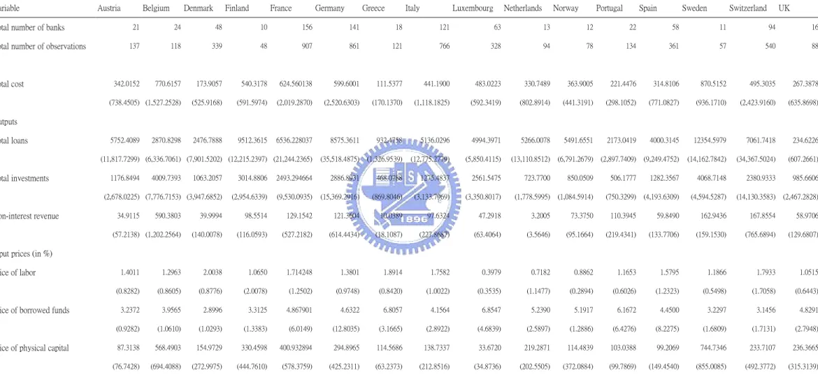
are the sum of the above three items of expenditure. Table 1 summarizes descriptive

statistics and the distributions of the sample banks among countries. These statistics

Table 1 : Descriptive statistics of dataset - country average.

Variable Austria Belgium Denmark Finland France Germany Greece Italy Luxembourg Netherlands Norway Portugal Spain Sweden Switzerland UK

Total number of banks 21 24 48 10 156 141 18 121 63 13 12 22 58 11 94 16

Total number of observations 137 118 339 48 907 861 121 766 328 94 78 134 361 57 540 88

Total cost 342.0152 770.6157 173.9057 540.3178 624.560138 599.6001 111.5377 441.1900 483.0223 330.7489 363.9005 221.4476 314.8106 870.5152 495.3035 267.3878 (738.4505) (1,527.2528) (525.9168) (591.5974) (2,019.2870) (2,520.6303) (170.1370) (1,118.1825) (592.3419) (802.8914) (441.3191) (298.1052) (771.0827) (936.1710) (2,423.9160) (635.8698) Outputs Total loans 5752.4089 2870.8298 2476.7888 9512.3615 6536.228037 8575.3611 932.4758 5136.0296 4994.3971 5266.0078 5491.6551 2173.0419 4000.3145 12354.5979 7061.7418 234.6226 (11,817.7299) (6,336.7061) (7,901.5202) (12,215.2397) (21,244.2365) (35,518.4875) (1,326.9539) (12,775.2779) (5,850.4115) (13,110.8512) (6,791.2679) (2,897.7409) (9,249.4752) (14,162.7842) (34,367.5024) (607.2661) Total investments 1176.8494 4009.7393 1063.2057 3014.8806 2493.294664 2886.8931 468.0788 1275.4837 2561.5475 723.7700 850.0509 506.1777 1282.3567 4068.7148 2380.9333 985.6606 (2,678.0225) (7,776.7153) (3,947.6852) (2,954.6339) (9,530.0935) (15,369.2916) (869.8046) (3,133.7969) (3,350.8017) (1,778.5995) (1,084.5914) (750.3299) (4,193.6309) (4,594.5287) (14,130.3583) (2,467.2828) Non-interest revenue 34.9115 590.3803 39.9994 98.5514 129.1542 121.3604 10.0389 97.6324 47.2918 3.2005 73.3750 110.3945 59.8490 162.9436 167.8554 58.9706 (57.2138) (1,202.2564) (140.0078) (116.0593) (527.2182) (614.4434) (18.1087) (227.8687) (63.4064) (3.5646) (95.1664) (219.4341) (133.7706) (159.1530) (765.6894) (129.6807)

Input prices (in %)

Price of labor 1.4011 1.2963 2.0038 1.0650 1.714248 1.3801 1.8914 1.7582 0.3979 0.7182 0.8862 1.1653 1.5795 1.1866 1.7933 1.0515

(0.8282) (0.8605) (0.8776) (2.0078) (1.2502) (0.9748) (0.8420) (1.0022) (0.3535) (1.1477) (0.2894) (0.6026) (1.2323) (0.5498) (1.7058) (0.6443)

Price of borrowed funds 3.2372 3.9565 2.8996 3.3125 4.867901 4.6322 6.8057 4.1564 6.8547 5.2390 5.1917 6.1672 4.4500 3.2297 3.1456 4.8291

(0.9282) (1.0610) (1.0293) (1.3383) (6.0149) (12.8035) (3.1665) (2.8922) (4.6839) (2.5897) (1.2886) (6.4276) (8.2275) (1.6809) (1.7131) (2.7948)

Price of physical capital 87.3138 568.4903 154.9729 330.4598 400.932894 294.8965 114.5686 138.7337 33.6720 219.2871 114.4839 103.0388 99.2069 744.7346 233.7107 236.3665

(76.7428) (694.4088) (272.9975) (444.7610) (578.3759) (425.2311) (63.2373) (212.8516) (34.8736) (202.5505) (372.0884) (99.7869) (149.4540) (855.0085) (492.3772) (315.3139)

5. Empirical Results

5.1 Parameter Estimates

Each country’s cost frontier is estimated by the model developed by Battese and

Coelli (1992). A standard translog cost function with trends is expressed as

∑∑

∑

∑

= = = = + + + = 4 1 4 1 3 1 4 1 0 ln ln 2 1 ln ln ln j m mwt jwt jm k kwt k j jwt j wt Y W Y Y C

α

α

β

γ

wt wt j k kwt jwt jk k n nwt kwt kn W W + Y W +U +V +

_∑∑

_∑∑

= = = = 4 1 3 1 3 1 3 1 ln ln ln ln 2 1

δ

ρ

(17)

where U_wt denotes the production inefficiency and is further specified as

(

)

[

]

{

}

w wt t T U U = exp−

η

− . (18) wt

C is the real total costs for the bank w at time t, Y1 is the loans, Y2 is the

investments, Y3 is the non-interest revenues, Y4 is the linear time trend, W1 is the

price of labor, W2 is the price of physical capital, W3 is the price of borrowed funds,

wt

V is identically and independently distributed normal random variables with mean

zero and constant variance σ2 ν, and Uw is assumed to be a truncated normal

distribution as N+( µ, σu2 ). Both Vwt and Uw are mutually independent.

There are a few characteristics deserving specific mention. Microeconomic

theory requires that a cost function must have some properties. For example, a cost

function is homogeneous of first degree in input prices; it is symmetrical, i.e.,

mj jm

γ

γ

= (for all j≠m) and

δ

_kn =

δ

_nk(for all k≠n). Other properties can be checked after the parameters have been estimated. For estimation convenience, we transform

∑ ∑

∑

∑

= = = = + + + = 4 1 4 1 3 2 * 4 1 0 * ln ln 2 1 ln ln ln j m mwt jwt jm k kwt k j jwt j wt Y W Y Y C α α β γ wt wt j k kwt jwt jk k n nwt kwt kn W W + Y W +U +V +

∑∑

∑∑

= = = = 4 1 3 2 * 3 2 3 2 * * ln ln ln ln 2 1

δ

ρ

(19) wherelnC_wt* =lnC_wt −lnW_1wt, ln_W* ₌ln_{W −}ln_W1 ,_{k =}2,3 wt kwt kwt , and * lnW_nwt is similarly defined. In other words, the first input is arbitrarily chosen as the numeraire

and its price is used to normalize all the terms involving C, W2, and W3. Thus, theα,

β,γ,δ,ρ,η,µ,σ2 ν and σu2 are unknown parameters to be estimated. Table 2 reports

estimation results of each country based on equation (19) using the FRONTIER 4.1

program (Coelli, 1996).

The translog cost function is known as flexible, in the sense that it provides a

second-order approximation to the true function. Taking these estimated parameters as

given, we can examine whether the estimated cost function is concave in input prices.

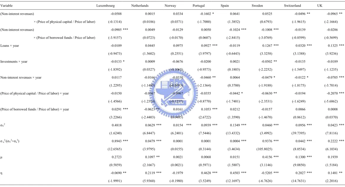
Particularly, the Hessian matrix requires H₁ ≤0, H₂ ≥0, and H₃ ≤0, where the Hessian matrices are defined as

0 11 1 = ≤ ∗ C H ， 0 22 21 12 11 2 = ∗ ∗ ≥ ∗ ∗ C C C C H ， 0 33 32 31 23 22 21 13 12 11 3 = ≤ ∗ ∗ ∗ ∗ ∗ ∗ ∗ ∗ ∗ C C C C C C C C C H (20) where n k kn W W C C ∂ ∂ ∂ = ∗ 2 ,∀ nk, =1,2,3.

Next, according Shephard’s Lemma, an input share is equal to the derivative of the

log cost function with respect to that log input price. Each input share should lie in

zero and unity, and adds up to 1, i.e.,

1 ln ln 0 < ∂ ∂ = < k k W C S ,k=1,2,3, and 1 3 1 =

∑

= k k S . (21)

0 > ∂ ∂ = j j Y C MC ， j=1,2,3 (22) Table 3 summarizes the above calculations based on equations (20) through (22). It

reports the number of sample points inconsistent with the theory. Most of the

observations satisfy the stated properties, although there are some observations

against the requirements. In their recent survey on the estimation of the cost function,

Greene et al. (2004) have given some explanations for this problem. It may come

from that the share equations are not simultaneously estimated. However, the translog

cost function is largely congruent with the theory and hence well-representative.

Having estimated and analyzed each country’s cost frontier, one may ask

whether all countries’ banks are operating under a unique type of technology or not. If

all banks share the same technology, it would be unnecessary to analyze data by a

meta-frontier model. A likelihood-ratio (LR) test of the null hypothesis that all

countries’ stochastic cost frontiers are the same is performed. We compare the sum of

the values of the log-likelihood functions for the stochastic cost frontiers for sixteen

countries with the value of the log-likelihood function for the stochastic cost frontier

estimated by pooling all the data. The value of the LR statistic amounts to 2295. The

null hypothesis is strongly rejected.4 Now that we are sure that each country’s banks

operate under different technology, the next step is to calculate a meta-frontier

function.

In order to compare the meta-frontier function with the conventional studies,

where the banking efficiencies are evaluated by simply pooling all the data across

countries without considering the technical difference, we also estimate the translog

4

The degrees of freedom of the LR statistic’s Chi-square distribution are 480, the difference between the number of parameters estimated under the null hypothesis and the alternative hypothesis.

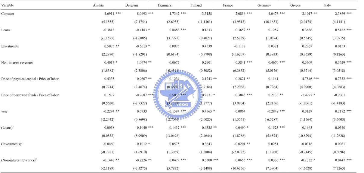
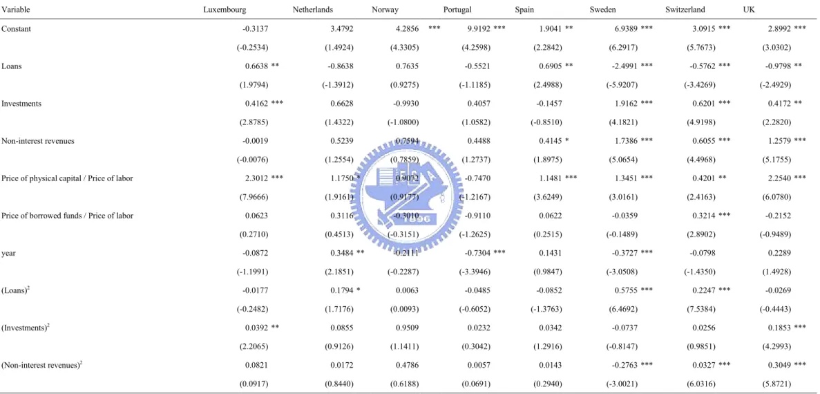
Table 2 : Estimation results of stochastic cost frontier

Variable Austria Belgium Denmark Finland France Germany Greece Italy

Constant 4.6911 *** 8.0493 *** 1.7342 *** -3.5158 2.0856 *** 4.0476 *** 2.1017 ** 2.3869 *** (5.1555) (7.1754) (2.6935) (-1.1361) (3.9513) (10.1633) (2.0174) (4.1141) Loans -0.3818 -0.4183 * 0.8486 *** 0.1633 0.3657 ** 0.1257 0.3836 0.5182 *** (-1.1575) (-1.6885) (3.7977) (0.4021) (2.5289) (1.0874) (0.5345) (3.0715) Investments 0.5075 ** -0.5613 * 0.0975 0.4539 -0.1178 0.0321 0.2767 0.0153 (2.2870) (-1.8291) (0.6194) (0.9798) (-1.6207) (0.3933) (0.3659) (0.1265) Non-interest revenues 0.4017 * 1.0674 ** -0.0677 0.2901 0.5841 *** 0.4670 *** 0.3609 0.3629 *** (1.8382) (2.3806) (-0.4391) (0.5052) (6.3832) (5.0176) (0.5714) (3.0518)

Price of physical capital / Price of labor 0.4333 0.9607 ** 0.1234 2.1243 ** 0.2821 ** 0.1141 4.7546 *** 0.7332 ***

(0.7744) (2.4674) (0.4660) (2.9184) (2.2968) (0.7264) (4.0900) (4.0883)

Price of borrowed funds / Price of labor 0.1577 -0.7687 *** 0.5035 *** 0.9271 * 0.3845 *** 0.2133 ** -1.4797 * -0.2061

(0.5620) (-2.7322) (3.1388) (1.8777) (3.9904) (2.2156) (-1.8061) (-1.4183) year -0.2294 ** 0.0733 -0.1584 *** 0.4565 * 0.0864 -0.2848 *** 0.3129 0.2172 *** (-2.2442) (0.8698) (-2.7060) (2.0025) (1.3561) (-6.5287) (1.1764) (3.5603) (Loans)2 _{0.0058 0.1040 *** -0.1437 *** 0.4335 ** 0.0490 * 0.1523 *** -0.1663 -0.0340} (0.0532) (5.9909) (-3.0498) (2.4644) (1.8788) (5.4574) (-0.8294) (-1.2628) (Investments)2 _{-0.0460 0.1012 * 0.0575 0.3643 -0.0201 ** 0.0251 -0.0316 0.0061} (-0.7781) (1.6910) (1.3039) (1.3804) (-2.0722) (1.1960) (-0.2445) (0.3096) (Non-interest revenues)2 _{-0.1448 ** -0.2226 ** 0.0479 *** 0.3300 *** 0.0655 *** 0.0336 *** -0.1332 * 0.0447 ***} (-2.1189) (-2.3275) (5.7822) (3.2488) (10.6256) (7.3904) (-1.6628) (7.3265)

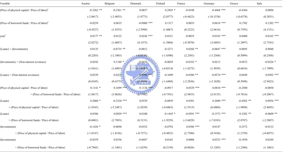
Table 2 : Estimation results of stochastic cost frontier (continued)

Variable Austria Belgium Denmark Finland France Germany Greece Italy

(Price of physical capital / Price of labor)2 _{-0.3262 ** -0.2361 ** 0.0857 0.2845 * -0.0108 -0.4468 *** -0.4384 0.0094}

(-2.0617) (-2.4055) (1.0773) (2.0377) (-0.4423) (-10.1538) (-0.6378) (0.2031)

(Price of borrowed funds / Price of labor)2 _{-0.0259 0.0635 -0.0900 *** 0.1317 0.0035 0.0618 *** 0.1702 0.1202 ***}

(-0.4527) (1.4255) (-2.5998) (1.6067) (0.2223) (2.6616) (0.7393) (4.1351)

year2 _{0.0177 ** 0.0122 0.0244 *** 0.0321 -0.0035 0.0183 *** 0.0400 0.0165 ***}

(2.0272) (1.6047) (4.1473) (1.5804) (-0.5070) (3.6885) (1.2897) (2.7543)

(Loans) × (Investments) 0.0135 -0.0735 ** -0.0012 -0.3271 0.0266 ** -0.0647 *** 0.0695 0.0048

(0.2203) (-2.1065) (-0.0338) (-1.6500) (2.2301) (-3.2568) (0.5099) (0.2568)

(Investments) × (Non-interest revenues) 0.0542 0.1180 * -0.0436 -0.0029 -0.0183 * 0.0213 0.0472 -0.0226 *

(1.0161) (1.6903) (-1.4490) (-0.0314) (-1.8275) (1.4939) (0.6018) (-1.7099)

(Loans) × (Non-interest revenues) 0.0539 0.0225 0.0996 *** -0.1609 -0.0306 ** -0.0374 *** 0.0449 0.0502 ***

(0.6345) (0.6375) (3.3959) (-1.6488) (-2.2836) (-2.1820) (0.3948) (2.9423)

(Price of physical capital / Price of labor) 0.1141 * 0.1699 *** 0.1134 *** -0.0917 0.0529 *** 0.0810 *** -0.2500 -0.0058

× (Price of borrowed funds / Price of labor) (1.6817) (3.0626) (2.7782) (-0.7541) (2.9833) (2.8135) (-0.7816) (-0.2067)

(Loans) 0.2060 * -0.2320 *** 0.0539 -0.0859 0.0301 0.2690 *** -0.4502 ** 0.0936 ***

× (Price of physical capital / Price of labor) (1.8345) (-5.2487) (1.0259) (-0.6863) (1.5515) (8.6084) (-1.9898) (2.8695)

(Loans) 0.0386 0.0929 *** 0.0100 -0.1445 * -0.0591 *** -0.1573 *** 0.3302 ** -0.0609 **

× (Price of borrowed funds / Price of labor) (0.6081) (2.7893) (0.3131) (-1.9529) (-3.6829) (-7.8183) (2.0787) (-2.2807)

(Investments) -0.1426 * -0.0696 -0.0352 -0.0792 0.0386 *** 0.0147 0.2572 -0.0133

× (Price of physical capital / Price of labor) (-1.8147) (-1.4156) (-0.7371) (-0.4852) (2.7580) (0.5436) (1.2759) (-0.6075)

(Investments) -0.0359 0.0356 -0.0447 0.0165 0.0008 0.0523 *** -0.1930 0.0244

× (Price of borrowed funds / Price of labor) (-0.7945) (1.1401) (-1.6259) (0.2139) (0.0826) (3.1285) (-1.2306) (1.1863)

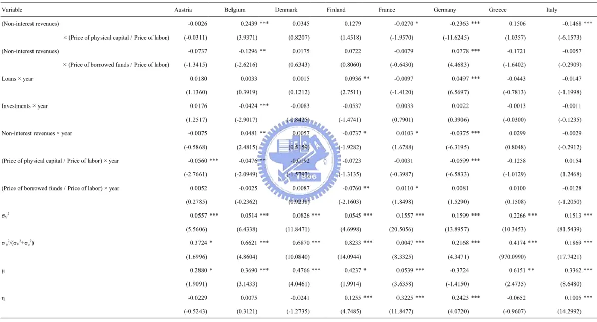
Table 2 : Estimation results of stochastic cost frontier (continued)

Variable Austria Belgium Denmark Finland France Germany Greece Italy

(Non-interest revenues) -0.0026 0.2439 *** 0.0345 0.1279 -0.0270 * -0.2363 *** 0.1506 -0.1468 ***

× (Price of physical capital / Price of labor) (-0.0311) (3.9371) (0.8207) (1.4518) (-1.9570) (-11.6245) (1.0357) (-6.1573)

(Non-interest revenues) -0.0737 -0.1296 ** 0.0175 0.0722 -0.0079 0.0778 *** -0.1721 -0.0057

× (Price of borrowed funds / Price of labor) (-1.3415) (-2.6216) (0.6343) (0.8060) (-0.6430) (4.4683) (-1.6402) (-0.2909)

Loans × year 0.0180 0.0033 0.0015 0.0936 ** -0.0097 0.0497 *** -0.0443 -0.0147

(1.1360) (0.3919) (0.1212) (2.7511) (-1.4120) (6.5697) (-0.7813) (-1.1998)

Investments × year 0.0176 -0.0424 *** -0.0083 -0.0537 0.0033 0.0022 -0.0013 -0.0011

(1.2517) (-2.9017) (-0.8425) (-1.4741) (0.7901) (0.3906) (-0.0300) (-0.1235)

Non-interest revenues × year -0.0075 0.0481 ** 0.0057 -0.0737 * 0.0103 * -0.0375 *** 0.0299 -0.0029

(-0.5868) (2.4815) (0.5159) (-1.9282) (1.6788) (-6.3195) (0.8048) (-0.2912)

(Price of physical capital / Price of labor) × year -0.0560 *** -0.0476 ** -0.0192 -0.0723 -0.0031 -0.0599 *** -0.1258 0.0154

(-2.7661) (-2.0949) (-1.5797) (-1.3135) (-0.3987) (-6.5833) (-1.0129) (1.2468)

(Price of borrowed funds / Price of labor) × year 0.0052 -0.0025 0.0087 -0.0760 ** 0.0110 * 0.0081 0.0100 -0.0128

(0.2785) (-0.2362) (0.9238) (-2.1603) (1.8498) (1.5290) (0.1508) (-1.2050) σV2 0.0557 *** 0.0514 *** 0.0826 *** 0.0545 *** 0.1557 *** 0.1599 *** 0.2266 *** 0.1513 *** (5.5606) (6.4338) (11.8471) (4.6998) (20.5056) (13.8957) (10.3453) (81.5439) σ u2/(σV2+σu2) 0.3724 * 0.6621 *** 0.6870 *** 0.8233 *** 0.0047 *** 0.2168 *** 0.4174 *** 0.1869 *** (1.6996) (4.8604) (10.0840) (14.0944) (8.3325) (4.3471) (970.0990) (17.7421) µ 0.2880 * 0.3690 *** 0.4766 *** 0.4237 * 0.0539 *** -0.3724 0.6151 ** 0.3362 *** (1.9091) (3.1433) (4.0461) (1.9914) (3.6358) (-1.4150) (2.4735) (8.6480) η -0.0229 0.0075 -0.0241 0.1255 *** 0.3225 *** 0.2423 *** -0.0652 0.1005 *** (-0.5243) (0.3121) (-1.2735) (4.7485) (11.8477) (4.0720) (-0.9607) (14.2992)

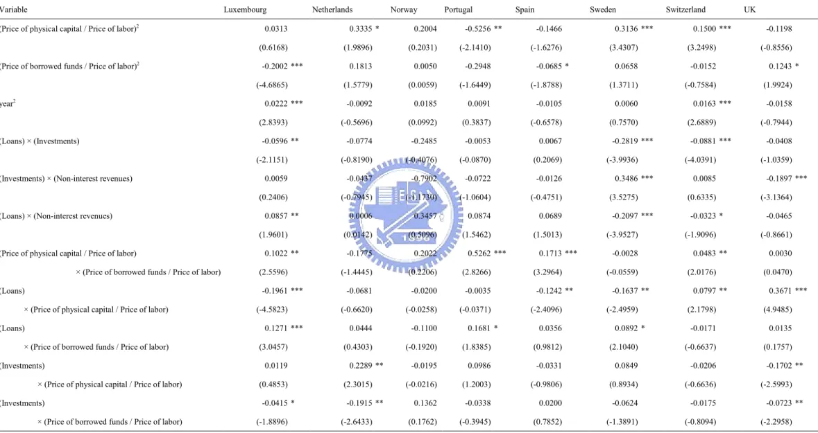
Table 2 : Estimation results of stochastic cost frontier (continued)

Variable Luxembourg Netherlands Norway Portugal Spain Sweden Switzerland UK

Constant -0.3137 3.4792 4.2856 *** 9.9192 *** 1.9041 ** 6.9389 *** 3.0915 *** 2.8992 *** (-0.2534) (1.4924) (4.3305) (4.2598) (2.2842) (6.2917) (5.7673) (3.0302) Loans 0.6638 ** -0.8638 0.7635 -0.5521 0.6905 ** -2.4991 *** -0.5762 *** -0.9798 ** (1.9794) (-1.3912) (0.9275) (-1.1185) (2.4988) (-5.9207) (-3.4269) (-2.4929) Investments 0.4162 *** 0.6628 -0.9930 0.4057 -0.1457 1.9162 *** 0.6201 *** 0.4172 ** (2.8785) (1.4322) (-1.0800) (1.0582) (-0.8510) (4.1821) (4.9198) (2.2820) Non-interest revenues -0.0019 0.5239 0.7594 0.4488 0.4145 * 1.7386 *** 0.6055 *** 1.2579 *** (-0.0076) (1.2554) (0.7859) (1.2737) (1.8975) (5.0654) (4.4968) (5.1755)

Price of physical capital / Price of labor 2.3012 *** 1.1750 * 0.9072 -0.7470 1.1481 *** 1.3451 *** 0.4201 ** 2.2540 ***

(7.9666) (1.9161) (0.9177) (-1.2167) (3.6249) (3.0161) (2.4163) (6.0780)

Price of borrowed funds / Price of labor 0.0623 0.3116 -0.3010 -0.9110 0.0622 -0.0359 0.3214 *** -0.2152

(0.2710) (0.4513) (-0.3151) (-1.2625) (0.2515) (-0.1489) (2.8902) (-0.9489) year -0.0872 0.3484 ** -0.2111 -0.7304 *** 0.1431 -0.3727 *** -0.0798 0.2289 (-1.1991) (2.1851) (-0.2287) (-3.3946) (0.9847) (-3.0508) (-1.4350) (1.4928) (Loans)2 _{-0.0177 0.1794 * 0.0063 -0.0485 -0.0852 0.5755 *** 0.2247 *** -0.0269} (-0.2482) (1.7176) (0.0093) (-0.6052) (-1.3763) (6.4692) (7.5384) (-0.4443) (Investments)2 _{0.0392 ** 0.0855 0.9509 0.0232 0.0342 -0.0737 0.0256 0.1853 ***} (2.2065) (0.9126) (1.1411) (0.3042) (1.2916) (-0.8147) (0.9851) (4.2993) (Non-interest revenues)2 _{0.0821 0.0172 0.4786 0.0057 0.0143 -0.2763 *** 0.0327 *** 0.3049 ***} (0.0917) (0.8440) (0.6188) (0.0691) (0.2940) (-3.0021) (6.0316) (5.8721)

Table 2 : Estimation results of stochastic cost frontier (continued)

Variable Luxembourg Netherlands Norway Portugal Spain Sweden Switzerland UK

(Price of physical capital / Price of labor)2 _{0.0313 0.3335 * 0.2004 -0.5256 ** -0.1466 0.3136 *** 0.1500 *** -0.1198}

(0.6168) (1.9896) (0.2031) (-2.1410) (-1.6276) (3.4307) (3.2498) (-0.8556)

(Price of borrowed funds / Price of labor)2 _{-0.2002 *** 0.1813 0.0050 -0.2948 -0.0685 * 0.0658 -0.0152 0.1243 *}

(-4.6865) (1.5779) (0.0059) (-1.6449) (-1.8788) (1.3711) (-0.7584) (1.9924)

year2 _{0.0222 *** -0.0092 0.0185 0.0091 -0.0105 0.0060 0.0163 *** -0.0158}

(2.8393) (-0.5696) (0.0992) (0.3837) (-0.6578) (0.7570) (2.6889) (-0.7944)

(Loans) × (Investments) -0.0596 ** -0.0774 -0.2485 -0.0053 0.0067 -0.2819 *** -0.0881 *** -0.0408

(-2.1151) (-0.8190) (-0.4076) (-0.0870) (0.2069) (-3.9936) (-4.0391) (-1.0359)

(Investments) × (Non-interest revenues) 0.0059 -0.0437 -0.7902 -0.0722 -0.0126 0.3486 *** 0.0085 -0.1897 ***

(0.2406) (-0.7945) (-1.1730) (-1.0604) (-0.4751) (3.5275) (0.6335) (-3.1364)

(Loans) × (Non-interest revenues) 0.0857 ** 0.0006 0.3457 0.0874 0.0689 -0.2097 *** -0.0323 * -0.0465

(1.9601) (0.0142) (0.5096) (1.5462) (1.5013) (-3.9527) (-1.9096) (-0.8661)

(Price of physical capital / Price of labor) 0.1022 ** -0.1775 0.2022 0.5262 *** 0.1713 *** -0.0028 0.0483 ** 0.0030

× (Price of borrowed funds / Price of labor) (2.5596) (-1.4445) (0.2206) (2.8266) (3.2964) (-0.0559) (2.0176) (0.0470)

(Loans) -0.1961 *** -0.0681 -0.0200 -0.0035 -0.1242 ** -0.1637 ** 0.0797 ** 0.3671 ***

× (Price of physical capital / Price of labor) (-4.5823) (-0.6620) (-0.0258) (-0.0371) (-2.4096) (-2.4959) (2.1798) (4.9485)

(Loans) 0.1271 *** 0.0444 -0.1100 0.1681 * 0.0356 0.0892 * -0.0171 0.0135

× (Price of borrowed funds / Price of labor) (3.0457) (0.4303) (-0.1920) (1.8385) (0.9812) (2.1040) (-0.6637) (0.1757)

(Investments) 0.0119 0.2289 ** -0.0195 0.0986 -0.0331 0.0849 -0.0206 -0.1702 **

× (Price of physical capital / Price of labor) (0.4853) (2.3015) (-0.0216) (1.2003) (-0.9806) (0.8934) (-0.6636) (-2.5993)

(Investments) -0.0415 * -0.1915 ** 0.1362 -0.0338 0.0200 -0.0624 -0.0175 -0.0723 **

× (Price of borrowed funds / Price of labor) (-1.8896) (-2.6433) (0.1762) (-0.3945) (0.7852) (-1.3891) (-0.8094) (-2.2958)

Table 2 : Estimation results of stochastic cost frontier (continued)

Variable Luxembourg Netherlands Norway Portugal Spain Sweden Switzerland UK

(Non-interest revenues) -0.0588 0.0015 0.0334 -0.1602 * 0.0641 0.0525 -0.0496 ** -0.0965 **

× (Price of physical capital / Price of labor) (-0.1314) (0.0186) (0.0371) (-1.7000) (1.3852) (0.6793) (-1.9615) (-2.1664)

(Non-interest revenues) -0.0905 *** 0.0049 -0.0129 0.0050 -0.1024 *** -0.1008 *** -0.0139 -0.0286

× (Price of borrowed funds / Price of labor) (-3.9157) (0.0723) (-0.0170) (0.0607) (-2.8415) (-3.0769) (-0.8599) (-0.5699)

Loans × year -0.0109 0.0445 0.0975 0.0927 *** -0.0119 0.1267 *** 0.0320 *** 0.1325 ***

(-0.9473) (1.5602) (0.2551) (3.9797) (-0.6443) (3.3258) (3.1388) (3.9236)

Investments × year -0.0133 * 0.0009 -0.0676 -0.0200 0.0021 -0.0502 ** -0.0135 -0.0189

(-1.8392) (0.0327) (-0.1065) (-0.9573) (0.1803) (-2.2252) (-1.5497) (-1.1235)

Non-interest revenues × year 0.0117 -0.0166 -0.0330 -0.0460 ** 0.0064 -0.0479 * -0.0122 * -0.0705 ***

(1.2295) (-1.1495) (-0.0593) (-2.1364) (0.3700) (-1.9188) (-1.8175) (-3.7014)

(Price of physical capital / Price of labor) × year -0.0150 -0.0367 -0.0967 -0.0355 -0.0442 * -0.0630 ** -0.0194 -0.2070 ***

(-1.4566) (-1.2314) (-0.1237) (-0.8770) (-1.7401) (-2.3531) (-1.6249) (-5.6862)

(Price of borrowed funds / Price of labor) × year 0.0291 *** -0.0623 ** 0.0161 0.1053 *** 0.0212 -0.0157 0.0066 0.0008

(3.2266) (-2.4403) (0.0485) (2.6722) (1.3590) (-1.4670) (0.8612) (0.0370) σV2 0.4818 0.0629 *** 0.0154 *** 0.0939 *** 0.1349 *** 0.0460 *** 0.0956 *** 0.0423 *** (1.6240) (6.8447) (6.2401) (7.5446) (13.4332) (3.4992) (39.7395) (7.8116) σ u2/(σV2+σu2) 0.8943 *** 0.0479 *** 0.0001 0.0001 0.0004 *** 0.9376 *** 0.0442 *** 0.2222 *** (12.6565) (3.9795) (0.0155) (0.3144) (3.4634) (105.8025) (8.0534) (6.1034) µ 0.2723 0.1097 ** 0.0021 0.0068 0.0151 0.4156 *** 0.1300 *** 0.1939 (0.5859) (2.1667) (0.0021) (0.5971) (1.5807) (3.1146) (9.0850) (1.5184) η -0.0690 ** 0.2119 *** -0.1979 0.4628 *** 0.4503 *** -0.5205 *** 0.2027 *** 0.1481 ** (-1.9991) (5.9360) (-0.1980) (3.5249) (12.1697) (-6.7626) (14.7631) (2.2016)

Table 3. Measures of regularity conditions on the stochastic frontier function S01 S02 S03 MC01 MC02 MC03 H1 H2 H3

country number ratio number ratio number ratio number ratio number ratio number ratio number ratio number ratio number ratio Austria 60 43.80% 45 32.85% 32 23.36% 3 2.19% 3 2.19% 3 2.19% 22 16.06% 67 48.91% 90 65.69% Belgium 19 16.10% 21 17.80% 56 47.46% 38 32.20% 47 39.83% 47 39.83% 74 62.71% 109 92.37% 56 47.46% Denmark 53 15.63% 40 11.80% 26 7.67% 3 0.88% 86 25.37% 86 25.37% 7 2.06% 287 84.66% 204 60.18% Finland 35 72.92% 21 43.75% 4 8.33% 14 29.17% 13 27.08% 13 27.08% 11 22.92% 42 87.50% 25 52.08% France 285 31.42% 140 15.44% 123 13.56% 0 0.00% 594 65.49% 594 65.49% 129 14.22% 683 75.30% 620 68.36% Germany 427 49.59% 314 36.47% 234 27.18% 15 1.74% 140 16.26% 140 16.26% 378 43.90% 635 73.75% 495 57.49% Greece 47 38.84% 63 52.07% 70 57.85% 41 33.88% 34 28.10% 34 28.10% 113 93.39% 106 87.60% 67 55.37% Italy 221 28.85% 288 37.60% 587 76.63% 20 2.61% 0 0.00% 0 0.00% 721 94.13% 581 75.85% 483 63.05% Luxembourg 253 77.13% 197 60.06% 105 32.01% 39 11.89% 137 41.77% 137 41.77% 44 13.41% 268 81.71% 159 48.48% Netherlands 83 88.30% 79 84.04% 44 46.81% 13 13.83% 43 45.74% 43 45.74% 67 71.28% 34 36.17% 48 51.06% Norway 67 85.90% 68 87.18% 25 32.05% 5 6.41% 46 58.97% 46 58.97% 25 32.05% 58 74.36% 46 58.97% Portugal 15 11.19% 17 12.69% 41 30.60% 5 3.73% 21 15.67% 21 15.67% 12 8.96% 119 88.81% 71 52.99% Spain 56 15.51% 20 5.54% 40 11.08% 6 1.66% 26 7.20% 26 7.20% 11 3.05% 183 50.69% 211 58.45% Sweden 18 31.58% 10 17.54% 8 14.04% 9 15.79% 34 59.65% 34 59.65% 21 36.84% 41 71.93% 32 56.14% Switzerland 314 58.15% 259 47.96% 37 6.85% 13 2.41% 222 41.11% 222 41.11% 31 5.74% 476 88.15% 358 66.30% UK 57 64.77% 53 60.23% 30 34.09% 29 32.95% 46 52.27% 46 52.27% 53 60.23% 62 70.45% 49 55.68% TOTAL 2010 40.39% 1635 32.85% 1462 29.38% 253 5.08% 1492 29.98% 1492 29.98% 1719 34.54% 3751 75.37% 3014 60.56% Note: It reports numbers of inappropriate samples by country.

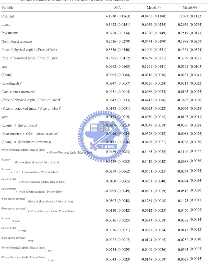
stochastic cost function for European banks at the same time.5 Table 4 reports the parameter

estimates obtained by the translog stochastic frontier cost function, meta-frontier linear

programming and quadratic programming. Standard errors of the estimators for the two

meta-frontier estimators are obtained by bootstrapping methods. Treating the sample as the

population, we randomly draw 1000 new datasets of the same size as sample with

replacement. For each generated dataset, the new meta-frontier parameters are estimated by

linear and quadratic programming. Therefore, there are 1000 suites of parameter estimates.

The estimated standard errors of the meta-frontier parameters are calculated as the standard

deviations of these 1000 sets of new parameters estimates. It is interesting to note that the LP

estimators do not significantly deviate from the QP estimators. However, there are substantial

differences between the meta-frontier coefficients and the corresponding coefficients of the

translog stochastic frontier. For the moment let us just confine our attention to LP estimators.

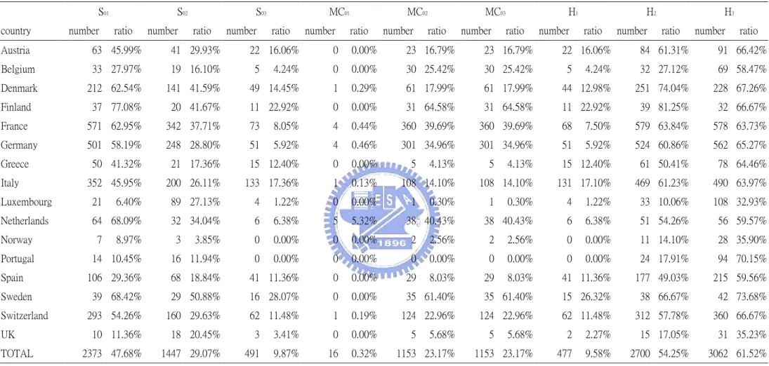
It may be worth pointing out, in passing, that the data would be improved on the

economic regularity conditions in the meta-frontier. In contrast to Table 3, Table 5 shows that

the percentages of the observations inconsistent with the regularity conditions decrease

substantially.

5

The translog stochastic frontier cost function for European is obtained by using the data of all banks under consideration.

Table 4: Maximum-likelihood estimates of the translog stochastic frontier for the selected European countries, along with the parameter estimates of the meta-frontier cost function.

Variable SFA Meta(LP) Meta(QP)

Constant 4.1930 (0.1763) -0.8465 (0.1180) 1.1093 (0.1122)

Loans -0.1422 (0.0451) 0.6059 (0.0234) 0.2639 (0.0244)

Investments 0.0728 (0.0334) 0.4320 (0.0149) 0.2519 (0.0173)

Non-interest revenues 0.2636 (0.0279) -0.0444 (0.0190) 0.1998 (0.0259)

Price of physical capital / Price of labor 0.5556 (0.0540) -0.1000 (0.0331) 0.4331 (0.0324)

Price of borrowed funds / Price of labor 0.2505 (0.0412) 0.6259 (0.0211) 0.3299 (0.0225)

year -0.0962 (0.0168) 0.1291 (0.0141) 0.0591 (0.0105) (Loans)2 0.0605 (0.0084) -0.0216 (0.0036) 0.0231 (0.0041) (Investments)2 0.0247 (0.0057) -0.0226 (0.0024) 0.0211 (0.0022) (Non-interest revenues)2 0.0451 (0.0014) -0.0086 (0.0024) 0.0165 (0.0025)

(Price of physical capital / Price of labor)2

0.0242 (0.0133) -0.4412 (0.0086) -0.3695 (0.0080)

(Price of borrowed funds / Price of labor)2

0.0148 (0.0081) -0.0023 (0.0022) 0.0064 (0.0028)

year2

0.0173 (0.0019) -0.0050 (0.0012) -0.0105 (0.0011)

(Loans) × (Investments) -0.0206 (0.0053) -0.0349 (0.0018) -0.0395 (0.0028)

(Investments) × (Non-interest revenues) 0.0096 (0.0034) 0.0328 (0.0022) 0.0081 (0.0025)

(Loans) × (Non-interest revenues) 0.0131 (0.0036) 0.0438 (0.0021) 0.0268 (0.0030)

(Price of physical capital / Price of labor)

× (Price of borrowed funds / Price of labor) 0.0489 (0.0083) 0.1465 (0.0035) 0.1140 (0.0032)

(Loans)

× (Price of physical capital / Price of labor) 0.0259 (0.0085) 0.1419 (0.0042) 0.0638 (0.0036)

(Loans)

× (Price of borrowed funds / Price of labor) -0.0259 (0.0062) -0.0553 (0.0025) -0.0244 (0.0024)

(Investments)

× (Price of physical capital / Price of labor) 0.0160 (0.0065) 0.0963 (0.0040) 0.0994 (0.0034)

(Investments)

× (Price of borrowed funds / Price of labor) -0.0209 (0.0049) -0.0601 (0.0019) -0.0518 (0.0020)

(Non-interest revenues)

×(Price of physical capital / Price of labor) -0.0507 (0.0048) -0.1781 (0.0018) -0.1425 (0.0017)

(Non-interest revenues)

× (Price of borrowed funds / Price of labor) 0.0110 (0.0042) 0.0612 (0.0025) 0.0470 (0.0022)

(Loans) × year -0.0016 (0.0025) 0.0243 (0.0018) 0.0288 (0.0014) (Investments) × year 0.0036 (0.0021) 0.0097 (0.0014) 0.0145 (0.0012) (Non-interest revenues) ×year -0.0022 (0.0017) -0.0194 (0.0015) -0.0252 (0.0010)

(Price of physical capital / Price of labor)

× year -0.0254 (0.0029) -0.0409 (0.0026) -0.0593 (0.0025)

(Price of borrowed funds / Price of labor)

Table 5. Measures of regularity conditions on the meta-frontier function S01 S02 S03 MC01 MC02 MC03 H1 H2 H3

country number ratio number ratio number ratio number ratio number ratio number ratio number ratio number ratio number ratio Austria 63 45.99% 41 29.93% 22 16.06% 0 0.00% 23 16.79% 23 16.79% 22 16.06% 84 61.31% 91 66.42% Belgium 33 27.97% 19 16.10% 5 4.24% 0 0.00% 30 25.42% 30 25.42% 5 4.24% 32 27.12% 69 58.47% Denmark 212 62.54% 141 41.59% 49 14.45% 1 0.29% 61 17.99% 61 17.99% 44 12.98% 251 74.04% 228 67.26% Finland 37 77.08% 20 41.67% 11 22.92% 0 0.00% 31 64.58% 31 64.58% 11 22.92% 39 81.25% 32 66.67% France 571 62.95% 342 37.71% 73 8.05% 4 0.44% 360 39.69% 360 39.69% 68 7.50% 579 63.84% 578 63.73% Germany 501 58.19% 248 28.80% 51 5.92% 4 0.46% 301 34.96% 301 34.96% 51 5.92% 524 60.86% 562 65.27% Greece 50 41.32% 21 17.36% 15 12.40% 0 0.00% 5 4.13% 5 4.13% 15 12.40% 61 50.41% 78 64.46% Italy 352 45.95% 200 26.11% 133 17.36% 1 0.13% 108 14.10% 108 14.10% 131 17.10% 469 61.23% 490 63.97% Luxembourg 21 6.40% 89 27.13% 4 1.22% 0 0.00% 1 0.30% 1 0.30% 4 1.22% 33 10.06% 108 32.93% Netherlands 64 68.09% 32 34.04% 6 6.38% 5 5.32% 38 40.43% 38 40.43% 6 6.38% 51 54.26% 56 59.57% Norway 7 8.97% 3 3.85% 0 0.00% 0 0.00% 2 2.56% 2 2.56% 0 0.00% 11 14.10% 28 35.90% Portugal 14 10.45% 16 11.94% 0 0.00% 0 0.00% 0 0.00% 0 0.00% 0 0.00% 24 17.91% 94 70.15% Spain 106 29.36% 68 18.84% 41 11.36% 0 0.00% 29 8.03% 29 8.03% 41 11.36% 177 49.03% 215 59.56% Sweden 39 68.42% 29 50.88% 16 28.07% 0 0.00% 35 61.40% 35 61.40% 15 26.32% 38 66.67% 42 73.68% Switzerland 293 54.26% 160 29.63% 62 11.48% 1 0.19% 124 22.96% 124 22.96% 62 11.48% 312 57.78% 360 66.67% UK 10 11.36% 18 20.45% 3 3.41% 0 0.00% 5 5.68% 5 5.68% 2 2.27% 15 17.05% 31 35.23% TOTAL 2373 47.68% 1447 29.07% 491 9.87% 16 0.32% 1153 23.17% 1153 23.17% 477 9.58% 2700 54.25% 3062 61.52% Note: It reports numbers of inappropriate samples by country.

5.2 Cost Efficiency and Technology Gap Ratio

In this section we shift our attention to the estimates of the cost efficiency and the

technology gap, calculated by applying the LP estimated parameters. Measures of the TGR,

along with the relative cost efficiency (CE) and the meta-frontier frontier (CE*), are

reported on Table 6. In terms of CE, the mean values range from 0.47 for Finland to 0.99 for

Norway, estimated from equation (7). These results imply that, on average, the potential

cost saving for Finland banks is about 53% of their actual costs, which may be attributed to

the managerial inefficiency. In contrast, banks in Norway, on average, almost lie on their

cost frontier. Overall, for the whole European Banking industry, the mean value of the CE is

about 0.71. This is consistent with the results which are found by Altunbas et al. (2001) and

Vennet (2002). However, the mean values of CE* vary from 0.06 for UK to 0.36 for

Germany. It is obvious that there are quite a few of banks operating far beyond the meta

cost frontier. It deserves to take a closer look at some important features of the technology

gap. The mean values of the TGR range from 0.1 for UK to 0.55 for Finland. This indicates

that the overall level of production technology adopted by the UK banks tends to be the

lowest among the sample countries, while the Finnish banks appear to employ superior

production process. It is interesting to note that most of the sample countries’ cost frontiers,

except for Denmark, Norway, Portugal, Sweden and UK, are tangent to the meta cost

frontier, as they all have the estimated values of TGR equaling unity.

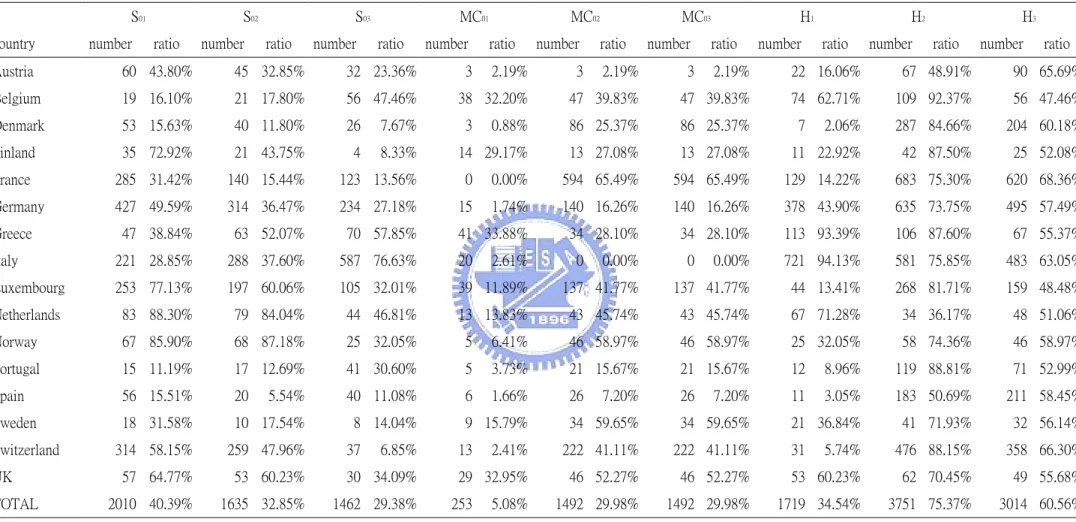
The frequency distributions for the technology gap ratios could give us more insights into

the technology difference among European countries. Figure 2 tells us that there is a good

deal of variability in the technology gap ratios for banks in all countries. We find that in many

countries banks adopt the inferior technology, since the frequency distributions for the

technology gap ratios are skew to the right. Banks in Germany own the highest mean cost

efficiencies relative to the meta-frontier. In contrast, banks in Norway have the highest cost

efficiencies (CE) relative to their stochastic frontier, while its average TGR estimate is low,

Table 6. Summary Statistics for TGRs and the cost efficiency measures for the sample countries

Country/Statistic Mean Minimum Maximum St. Dev. Country/Statistic Mean Minimum Maximum St. Dev.

Austria Luxembourg CE 0.7637 0.5514 0.9580 0.0811 CE 0.6188 0.1965 0.9468 0.2052 TGR 0.3568 0.0516 1.0000 0.1653 TGR 0.2221 0.0044 1.0000 0.1843 CE* 0.2715 0.0388 0.8247 0.1288 CE* 0.1336 0.0035 0.7638 0.1143 Belgium Netherlands CE 0.6585 0.4663 0.9518 0.1209 CE 0.6749 0.2397 0.9447 0.1775 TGR 0.4700 0.0251 1.0000 0.2212 TGR 0.3676 0.0003 1.0000 0.2363 CE* 0.3129 0.0143 0.7348 0.1686 CE* 0.2393 0.0002 0.8720 0.1768 Denmark Norway CE 0.6302 0.3321 0.9800 0.1391 CE 0.9989 0.9979 0.9996 0.0005 TGR 0.4804 0.0108 0.9695 0.1920 TGR 0.2709 0.1096 0.8955 0.1443 CE* 0.2926 0.0062 0.7201 0.1138 CE* 0.2706 0.1095 0.8942 0.1441 Finland Portugal CE 0.4731 0.0677 0.9048 0.2525 CE 0.9073 0.5174 0.9944 0.0975 TGR 0.5475 0.0941 1.0000 0.2668 TGR 0.3096 0.0800 0.8314 0.1349 CE* 0.2235 0.0327 0.5939 0.1215 CE* 0.2825 0.0795 0.8262 0.1336 France Spain CE 0.7452 0.1850 0.9857 0.1727 CE 0.8545 0.2048 0.9922 0.1424 TGR 0.4038 0.0005 1.0000 0.1415 TGR 0.3248 0.0277 1.0000 0.1184 CE* 0.3048 0.0003 0.9164 0.1371 CE* 0.2829 0.0266 0.9316 0.1214 Germany Sweden CE 0.8086 0.1118 0.9913 0.1421 CE 0.8653 0.5120 0.9960 0.1338 TGR 0.4290 0.0066 1.0000 0.1570 TGR 0.3955 0.0403 0.9855 0.2688 CE* 0.3551 0.0061 0.8203 0.1602 CE* 0.3159 0.0397 0.8004 0.1848 Greece Switzerland CE 0.6227 0.3805 0.9071 0.1268 CE 0.6967 0.2590 0.9757 0.1583 TGR 0.4532 0.0791 1.0000 0.1805 TGR 0.4767 0.0129 1.0000 0.1403 CE* 0.2854 0.0575 0.7311 0.1440 CE* 0.3355 0.0091 0.7716 0.1292 Italy UK CE 0.5598 0.1437 0.9668 0.1783 CE 0.6943 0.2768 0.9238 0.1333 TGR 0.5234 0.0096 1.0000 0.1603 TGR 0.0963 0.0032 0.2130 0.0589 CE* 0.2868 0.0089 0.7582 0.1150 CE* 0.0665 0.0025 0.1632 0.0432 Total CE 0.7145 0.0677 0.9996 0.1906 TGR 0.4140 0.0003 1.0000 0.1851 CE* 0.2919 0.0002 0.9316 0.1473

Austria Belgium Denmark Finland France Germany Greece Italy

Luxembourg Netherlands Norway Portugal Spain Sweden Switzerland UK Figure 2. Frequency distributions of TGRs in different countries (continued).

One may ask whether the relative cost efficiency scores are correlated with the

technology gap ratios. This information provides a potential link between technology

advancement and production efficiency levels. Figure 3 indicates that the two measures are

negatively associated with each other in a medium degree, with Luxembourg and UK

exhibiting larger variability. This indicates that in a country which faces swift technical

innovations (higher TGR) over time, banks may adopt such innovations in a tardy manner.

This type of rigidity hinders banks from optimally selecting input levels, due possibly to the

existence of quasi-fixed inputs, because they are incapable of adjusting instantly.

Having access to a panel of data incorporating both cross-sectional and time series

properties, we are able to analyze the relative cost efficiency and the technology gap ratio

over time. The relative cost efficiency scores and the technology gap ratios are averaged

across time, respectively. These figures help us understand the evolution of the measures for

the sample banks over time. Figure 4 shows that both CE and TGR gradually grow with time,

but the mean values of the TGR slightly decrease after 2001.

0 0.1 0.2 0.3 0.4 0.5 0.6 0.4 0.6 0.8 1 CE T G R

Austria Belgium Denmark

Finland France Germany

Greece Italy Luxembourg

Netherlands Norway Portugal

Spain Sweden Switzerland

UK