Sliding mode-based learning control for positioning of flying pickup head

Proceedings of the 2001 IEEE International Conference on Control Applications September 5-7,2001 Mexico City, Mexico

SLIDING MODE-BASED LEARNING CONTROL

FOR POSITIONING OF FLYING PICKUP HEAD

T.S.

L I U ~

W.C.

wul

Department of Mechanical Engineering, National Chiao Tung University, Hsinchu 300 1 0, TAIWAN, Department of Mechanical Engineering, National Chiao Tung University, Hsinchu 300 10, TAIWAN, V

R.O.C. [email protected] R.O.C.

Abstract. To deal with repetitive runout and disturbance in near-field optical disk drives, this study develops a sliding mode based learning controller. It incorporates characteristics of sliding mode control into learning control. The reason for using sliding mode control is attributed to robust properties dealing with model uncertainty and disturbances. The learning algorithm utilizes shape functions to approximate influence functions in integral transforms and estimate the control input to perform seeking movement. It learns at each sampling instant the desired control input without prior knowledge of system dynamics. To validate the proposed method, this work conducts track-seeking expei-iments.

Key Words: Disk Drive, Track Seeking, Sliding Mode Control, Learning Control.

1. INTRODUCTION

control input vector generated by actuators, M ( q ) is the symmetric positive definite generalized inertia

matrix, C ( q , q ) results from Coriolis and centripetal n e near-field optical disk drive as depicted in Fig. 1 is

a new generation optical disk drive design after digital versatile disk drives. It employs techniques of near- field optics, a flying pickup head, a solid immersion lens to achieve much higher optical data density recording. As a consequence, the control performances all need to be elevated since the data track width, track pitch, etc. get smaller. This paper presents a sliding

accelerations, G(q) is the generalized gravitational force vector, and d ( g ,

4)

denotes the disturbance. Define a state vector as

x =

[

3

=

[

;]

mode based learning scheme to eliminate repetitive

errors in optical disk drives. Eq. (1) can be written as

x

= A ( x )

+

B(x)u

+

v ( x )

2. SLIDING MODE BASED LEARNING

where CONTROL

I

x2 - M

-'

( x)C( X ) X ~

-

M -I ( X) G( X) A ( x ) = The equation of motion for a general system can be

expressed as

M ( q ) q + C(q,q>q + G ( q ) + d ( q , q ) = (1) are respectively the position, where q

,

q , and

and the disturbance is expressed by

0

- M

-'

( x ) d ( x )

2.1 Sliding Mode Control

A VCM is demanded to track a desired motion qd ( t )

.

Define an error vector

where e = q qd and i = q

gd

and hence a sliding variablt) s of the f o r b

r 1

where both and

r

are positive definite matrices. To execute the sliding mode control, there are many types of reaching laws proposed. The constant reaching speed form is the basic one that defined as

S =

Qsgn(s)

( 3 )

Simple is the advantage of this form, but obviously the value of Q must be well selected. The reaching time will be too long cause by small value of Q used, and too large value will induce chattering condition happening. In addition, a modified reaching law [I] is

defined as

i=-Qsgn(s)-Ks (4)

where gains Q and K are diagonal matrices with positive elements q, and k , , respectively. Chattering can be reduced by tuning q, and

k,

in this reaching law. Near the sliding surface, S ,

=

0 . It follows from Eq. ( 3 ) that IS,I 4,

.

By using a small gain, the chattering amplitude can be reduced. However, q, cannot be chosen equal to zero-since the reaching time would become infinite. Moreover, when the state is not

near the sliding surface a large k, is employed to increase the reaching rate.

Taking the time derivative of Eq. (2) gives

Equating Eqs. (3) and

(4)

yields control input

2.2 Sliding Mode Based Learning Control

Tracking control in this study is aimed at following a prescribed trajectory or eliminating a known frequency disturbance as closely as possible to improve the tracking performance. Using inverse kinematics one

can obtain position, velocity, and acceleration vectors denoted by 4 d' qd ' ' and

i d ,

respectively. The desired

control input of the VCM, denoted by w d ( . ) R _ j R"

,

is defined as

Definition: Let

c,

( T ) denote a subset of C ( T ) (which

is the space of continuous T-period functions

R " ) such that every wd is piecewise wd

'

R+

continuously differentiable, and

Given a collection for shape functions

{ai

and 0 ,

there exists a finite number of shape functions { @

,

@

,

,

@

,... ,

@ } that uniformly approximate members of C,(T) within 0

,

i.e. for every

wd E

C,(T)

,

there exists constant vectors

C,,,C,, C,

,...,

C, R" Such that

To estimate the desired control input wd ( t )

,

it can be approximated by a linear combination of appropriately selected period shape functions

The estimated

Gd

( t ) is hence indirectly updated by the adaptation of i ( t , )

,

which is the estimate of the influence function I ( )

.

i. Hence, N

W d ( t ) Z

c;

; ( t )

i o (7)

In the integral transform estimation, the feedforward term

Gd

( t ) is estimated through updating the influence function i ( t , ) according to the learning law Eq. (13). However, if the influence function, which belongs to the space of continuous T-period functions, satisfies SUP l ( 1 7 -

5

ei

( t 7

r)@i

(

r)/

,

it can be expressed by a set of shape functions. The unknown where Ci R" represent unknown coefficient vectors

for each shape function ; at an instant, and N denotes

the total number of shape functions. The estimated feedforward term is generated by determining the

coefficient vectors

e;

121, i.e., t d O , T l i o

The coefficient vectors are updated on-line by conducting the following estimation law [2]:

d -

-Ci(t) = -K, ,(t)s i = 1,2,...,N (9)

dt

where K , is a constant positive definite matrix. Another approximation of the ideal feedforward compensation term can be represented by

where the function K(o,o) Hilbert-Schmit kernel that satisfies

Rx[O,T] is a known

07K(t, )'d = k < K ( t , ) = K ( t + T , ) (11)

whereas the influence function I(.) [O,T]----,Rn is unknown. If a kernel function is chosen to satisfy Eq. (11), then the feedforward term w d ( t ) can be estimated by influence function I(.)

.

The following function adaptation law for estimating the unknown functions wd ( t ) and I(.) was presented by Messner et al. [3]:

influence function is proposed as

and the coefficient adaptation law becomes

d e i ( t , ) = -K,K(t,

)mi(

)S (15)

a t

where

mi(.)

denotes a shape function and

e;(.)

its associated coefficient.

Consider the plant defined in Eq. (l), a learning controller using sliding mode feedback control is proposed; i.e.

where

G d ( t )

can be estimated by the linear combination of shape functions Eq. (7) or by the integral of kernel function and influence function Eq. (12). The adaptation laws comprises Eqs. (8) and (15). 3. IMPLEMENTATION

As shown in Fig. 1, the near-field optical disk drive replaces the readwrite head in a hard disk drive by a solid immersion lens. Based on the model of a hard disk drive [4], the VCM transfer function reads

3.1 Sliding mode control

Sliding mode control employs the reaching law in Eq. (4) to valid the sliding surface design. Defining an error vector

where e =

7

-

qd

,

the s 'ding variable s is

'p

(18)

where A an& are positive. The reaching law in Eq. (4) can written as

s=-Qsgn s - K s = e + A e + T e = A e + T e + q - q d ) where Q and K are positive. From Eq. (1 7) that

the control input becomes

U =

M ,

[-

Qsgn

s

-

Ks

- Ae

- r e

+

q d }

(19) +

M2q

+ M39 where M ,

-

LmJ , M 2

-

K r K d r v r 3.2 Learning Control

Except for its employing shape functions to estimate influence functions, the structure of this learning control method is the same as learning control that using integral transforms. The learning control law consists of Eqs. (12), (14), and (15). There are some typical shape functions [2] such as Fourier series shape functions, polynomial shape functions, and piecewise linear shape functions, which can be used to

approximate the periodic continuous function I ( t , )

.

This study employs a set of piecewise linear functions, as depicted in Fig. 2. Accordingly, in each interval of

[ j/ N , ~ (i

+

1)T / N I , only two linear shape functions,

m i

and

m j

corresponding coefficients, cj and ci

,

,

to be updated at any instant. For computational efficiency of a kernel function, a piecewise linear function is used as a kernel function for integral transforms.

are required; i.e. there are only two

To implement the present method, Eqs. (12), (14), and (1 5) are rewritten to become the discretized form:

1 "

'

2 /=o

Gd(k)

=-

[K(k,I)j(k,I)+K(k,I+l)j(k,I+l)la

t (20)

k

ki(k,Z)

= k(k-l,I)-KLK(k,Z) i(I) s(i)At (22)

i k-a+l

where integral transforms are computed by a trapezoid method. Moreover, the sliding surface is formulated as

It follows from Eq. (23) that the control law Eq. (16) becomes, in discretized form,

~ ( k ) = -Qsgn[s(k)]

-

K [ s ( k ) ]

+

Gd

( E )

(24) In this discrete control algorithm,

k

represents an index for the feedback portion of the controller,

E

and I indexes for the learning portion, and a an integer that relates these indexes. For any given

k

in a period of the path, k ak a l . In other words, the adaptation parameters

2i

are updated at a rate a times slower than the inner feedback loop. Each increment in k represents a time step of At second, and each increment in

k

represents a time step of aAt second.

4. EXPERIMENTAL RESULTS

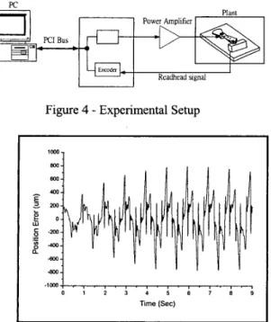
This study uses a digital optical readhead and an additional fan-shape component with reflective tape scale attached at one end of the suspension arm as shown in Fig. 3. The reflective tape scale in motion is scanned by a readhead. The readhead generates a digital square wave signal to the encoder in the NI PCI-

7344 FlexMotion control card as position feedback signals. Accordingly, the system resolution can achieve

0.1 m . Fig. 4 depicts this experimental setup.

From Eqs. (4) and (1 6), the sliding mode controller is defined as

U = Qsgn(s)

KS

and with the feedfonvard term the sliding mode based learning controller is defined as

I I

-

U =

-Q sgn(s)

-

Ks

+

W,

Flying Head

The value Q and K in both controllers are the same. Fig.

5 shows the off-track error in the sliding mode controller without learning control compensation. In contrast, Figs. 6 depicts the result of sliding mode based repetitive learning controller. Comparing results of Figs. 5 and 6 confirms that the sliding mode based repetitive learning controller indeed improves the repetitive motion accuracy better than the sliding mode controller.

In the presence of a sinusoidal disturbance, the sliding mode controller leads to results depicted in Fig. 7, which is inferior to those by the sliding mode based repetitive learning control method, as shown in Figs. 8

and 9. It is seen that the error amplitude is reduced with time, due to th feedforward input. The comparison between Figs. 8 and 9 demonstrates that the proper choice for learning coefficients

K ,

in Eq. (15) increases the error eliminating speed.

5. CONCLUSIONS

The present method yields error convergence faster than the sliding mode control method. Based on the property of learning control, the motion or disturbance period has to be known in advance to implement the proposed controller. Future study will combine adaptive control with the present method to overcome this limit.

6. FWFERNCES

[l] W. Gao, and J. C. Hung, 1993, “Variable

Structure Control of Nonlinear System: A New Approach”, IEEE Trans. on Industrial Electronics, Vol. 40, NO. 1, pp. 45-56.

[2] N. Sadegh, and K. Guglielmo, 1991, “A New repetitive Controller for Mechanical Manipulators”, Journal of Robotic System, Vol.

8,

No. 4, pp. 507-529.

[3] W. Messner, R. Horowitz, W. Kao, and M. Boals, 199 1, “A New Adaptive Learning Rule”,

IEEE

Transactions on Automatic Control, Vol. 36, No. 2,

pp. 188- 197.

[4] D. P. Magee, 1999, “Optimal Filtering to Improve Performance in Hard Disk Drive: Simulation

Results”, Proceedings of the American Control Conference, San Diego, California, pp. 71-75.

T

Deteclor

-

Rotation Disk

Figure 1

-

Flying head in optical system

o:k

, , , , , , ,

O - NT 1I N ?c N

...

T

t

O 2

t

Figure 2

-

Piecewise linear shape functions

Pan-shape component

Pr 1 Z W - tm- Plan[ Power Amplifier Readhead signal U

Figure 4

-

Experimental Setup

1m-,

-1md , , , , , , . , , , . , . , . , ,

,

0 1 2 3 4 5 6 7 8 9

Time (Sec)

Figure 5

-

Position error in sliding mode control

I

'3

1

1

, , , , , , , , , , , , , , , , .

,

-1Mxl

0 1 2 3 4 5 6 7 8 9

Time (Sec)

Figure 6 - Position error in sliding mode based learning control

I

Time (Sec)

I

Figure 7

-

Position error in sliding mode control with disturbance

'"7

Figure 8

-

Position error in sliding mode based learning control with learning coefficient

K , 200

Tine (Sec)

I

Figure 9

-

Position error in sliding mode based learning control with learning coefficient

K ,

400