適用於多輸入多輸出無線區域網路之適應性調變編碼及傳送模式選擇之跨層設計

國

立 交 通 大 學

電信工程學系碩士班

碩士論文

適用於多輸入多輸出無線區域網路之適應性

調變編碼及傳送模式選擇之跨層設計

Cross-Layer Design for Adaptive

Modulation/Coding and Transmission Mode

Selection over MIMO WLANs

研 究 生：楊松根 Student:

Sung-Kang

Yang

指導教授：李大嵩 博士 Advisor:

Dr.

Ta-Sung

Lee

適用於多輸入多輸出無線區域網路之適應性

調變編碼及傳送模式選擇之跨層設計

Cross-Layer Design for Adaptive Modulation/Coding and

Transmission Mode Selection over MIMO WLANs

研 究 生：楊松根 Student: Sung-Kang Yang

指導教授：李大嵩 博士 Advisor:

Dr. Ta-Sung Lee

國立交通大學

電信工程學系碩士班

碩士論文

A Thesis

Submitted to Institute of Communication Engineering

College of Electrical Engineering and Computer Science

National Chiao Tung University

in Partial Fulfillment of the Requirements

for the Degree of

Master of Science

in

Communication Engineering

June 2005

Hsinchu, Taiwan, Republic of China

適用於多輸入多輸出無線區域網路之適應性

調變編碼及傳送模式選擇之跨層設計

學生：楊松根

指導教授：李大嵩 博士

國立交通大學電信工程學系碩士班

摘要

多輸入多輸出(Multiple-Input Multiple-Output, MIMO)為使用多天線於傳送和 接收端的可靠通訊技術，並被認為是符合第四代高速通訊需求的最佳方案之一。 另一方面，正交分頻多工（Orthogonal Frequency Division Multiplexing, OFDM）為 一種具高頻譜效益，並能有效克服多路徑衰落效應的調變技術。在本論文中，吾 人針對MIMO-OFDM 提出一種跨層設計之適應性收發架構，使其能夠隨時間動態 地在頻率與空間通道上調整傳輸參數，如：調變階數、通道編碼以及傳輸能量， 吾人更進一步的透過同時考慮實體層與媒體存取層之共同設計，將MIMO 技術向 上延伸至媒體存取層，依據不同的品質要求，進行調整及修正系統參數與選用適 當的MIMO 傳輸技術，適切調整及修正重傳次數、封包長度、傳輸功率、傳輸速 率、調變型態等系統參數，以便充分地利用空間、時間以及頻率通道上的特性以 維持系統的目標錯誤率，達到最佳的性能。此種架構的特色之一在於可視需要彈 性地獲取多樣與多工兩種增益，且針對上層之需求根據通道狀況選擇適當之傳送 模式與參數。另外，不同的通道環境會造成不同的多路徑衰落效應。基於此一觀 點，吾人將探討結合智慧型天線與MIMO 之通訊系統架構，針對不同的環境效應， 選取最適合之傳輸技術。吾人將進一步針對MIMO 提出一種適應性傳收架構，以 便充分利用無線通道的特性。最後，吾人藉由電腦模擬驗證上述架構在室內無線 環境中具有優異的傳輸表現。

Cross-Layer Design for Adaptive

Modulation/Coding and Transmission Mode

Selection over MIMO WLANs

Student:

Sung-Kang

Yang

Advisor:

Dr.

Ta-Sung

Lee

Institute of Communication Engineering

National Chiao Tung University

Abstract

Multiple-input multiple-output (MIMO) is a promising technique suited to the increasing demand for high-performance 4G broadband wireless communications with multiple antennas at both transmitter and receiver side. In this thesis, we consider a new wireless communication system combining MIMO and OFDM, called the MIMO-OFDM system. To fully exploit the channel properties in the space-time-frequency wireless channels, we propose an adaptive MIMO-OFDM transceiver architecture along with a designed loading procedure to dynamically adjust the transmission parameters such as modulation order, channel coding and transmit power over spatial and frequency channels, according to the instantaneous channel statistics, to meet the target BER. Such transceiver scheme enjoys both the diversity and multiplexing gain in a flexible manner. Furthermore, we evaluate different error control and adaptation mechanisms available at different layers, namely MAC retransmission strategy, physical-layer channel coding, modulation order, MIMO mode, and adaptive packetization strategies. Besides, In a wireless transmission environment, the transmitted signal is scattered by various environmental objects causing different multi-path fading effects. With this point of view, we here consider a wireless communication system combining smart antenna or MIMO techniques. Depending on the channel condition, the optimal transmission technique is selected to combat channel impairments. Finally, we evaluate the performance of the proposed systems, and confirm that they work well in a typical indoor environment.

Acknowledgement

I would like to express my deepest gratitude to my advisor, Dr. Ta-Sung Lee, for his enthusiastic guidance and great patience. I learn a lot from his positive attitude in many areas. Heartfelt thanks are also offered to all members in the Communication Signal Processing (CSP) Lab for their constant encouragement. Finally, I would like to show my sincere thanks to my parents for their invaluable love.

Contents

Chinese Abstract

I

English Abstract

II

Acknowledgement III

Contents IV

List of Figures

VII

List of Tables

XII

Acronym Glossary

XIII

Notations XV

1 Introduction

1

2 MIMO

Techniques

Overview

5

2.1 Transmit/Receive Diversity: Concept and Technique... 5

2.2 Spatial Multiplexing: Concept and Technique... 8

2.2.1 Diagonal Bell Lab’s Layered Space-Time ...8

2.2.2 Vertical Bell Lab’s Layered Space-Time ...10

2.3 Review of OFDM ...14

2.4 V-BLAST Based OFDM...17

2.5.1 Generic Beamforming: Concept and Technique...18

2.5.2 Eigenbeamforming: Concept and Technique...19

2.6 Computer Simulations ...21

3 Adaptive Modulation Assisted MIMO-OFDM Systems

29

3.1 Adaptive Modulation ...30

3.2 SNR Based Switching Mechanism ...31

3.3 Adaptive MIMO-OFDM systems...32

3.4 Computer Simulations ...38

3.5 Summary...39

4 Cross-Layer Protection Strategies for AMC Over IEEE

802.11 MIMO WLANs

51

4.1 The Concept of Cross Layer Design...52

4.2 System Overview...53

4.2.1 Review of IEEE 802.11 MAC ...53

4.2.2 IEEE 802.11n Draft Overview...56

4.2.3 System Architecture of Proposed System...59

4.3 Throughput Efficiency and Delay Analysis...61

4.3.1 Average Frame Transmission Duration ...62

4.3.2 Delay Analysis ...64

4.4 Combining AMC and MAC Mechanisms ...64

4.4.1 System Performance Requirement at Physical Layer...65

4.4.2 Adaptive Packet Length Selection at MAC Layer...68

4.4.3 Physical/MAC Cross-Layer AMC Design...69

4.5 Computer Simulations ...70

5 MIMO Channel Condition and Transmission Strategies

86

5.1 MIMO Channel Model for IEEE 802.11n WLANs...88

5.1.1 MIMO Channel Model ...88

5.1.2 MIMO Channel Model for IEEE 802.11n WLANs...90

5.2 Determination of Channel Condition...92

5.3 Transmission Mode Selection Strategies ...93

5.3.1 Link-Optimal Space-Time Processing Based on Ergodic Capacity ....93

5.3.2 Analysis of IEEE 802.11n Channel Model...96

5.4 Summary...97

6 Conclusion

109

List of Figures

Figure 2.1 Diagram of a MIMO wireless transmission system...22 Figure 2.2 An illustration of a spatial multiplexing system ...22 Figure 2.4 Diagonal and Vertical Layered Space-Time encoding withN_t = ...23 3 Figure 2.5 Diagonal Layered Space-Time decoding withN_t = ...23 3 Figure 2.6 Vertical Layered Space-Time decoding withN_t = ...24 3 Figure 2.7 V-BLAST based MIMO-OFDM transmitter architecture. ...24 Figure 2.8 V-BLAST based MIMO-OFDM receiver architecture. ...25 Figure 2.9 Illustration of beamforming transceiver...25 Figure 2.10 ZF V-BLAST performance with ideal detection and cancellation.

QPSK modulation is used. (Nt, Nr) = (4, 4)...26 Figure 2.11 ZF V-BLAST performance with error propagation. (Nt, Nr ) = (4,

4). QPSK modulation is used...27 Figure 2.12 Comparison of ZF V-BLAST (Nt, Nr) = (4, 4) with QPSK

modulation and (Nt, Nr) = (2, 4) with 16-QAM modulation...28

Figure 3.1 A digital implementation of appending cyclic prefix into OFDM

signal in the transmitter...40 Figure 3.2 V-BLAST based MIMO-OFDM transmitter architecture. ...40 Figure 3.3 V-BLAST based MIMO-OFDM receiver architecture...41 Figure 3.4 A typical time and frequency selective fading channel. (By

assuming an exponential decay channel model with τ_rms =50 sn

and a speed of 15 m/s at 5 GHz)...41 Figure 3.5 BPSK, QPSK, 8-QAM, 16-QAM, 32-QAM, and 64-QAM

constellation diagrams. ...43 Figure 3.6 The average BER of various M-QAM modulation schemes over

AWGN channel...44 Figure 3.7 V-BLAST based adaptive MIMO-OFDM system transmitter

architecture...45 Figure 3.8 V-BLAST based adaptive MIMO-OFDM system receiver

architecture...45 Figure 3.9 The first stage bit loading procedure flow chart. ...46 Figure 3.10 Simulated probabilities of each modulation mode utilized by the

ZF V-BLAST based adaptive MIMO-OFDM system (with space loading) in the exponentially decay Rayleigh fading channel with

rms

τ =50 ns. 0 f_d = Hz. ( ,N N_{t r}) (4, 4)= ...47 Figure 3.11 Unutilized power ratio in the V-BLAST based adaptive

MIMO-OFDM system (with space-time loading) at different channel SNRs. Exponential decay Rayleigh fading channel with

50 s

rms n

τ = . 0 f_d = Hz . ( ,N N_{t r}) (4,5), (4,4), and (3,3)= .

Other parameters are listed in Table 3.3. ...48 Figure 3.12 BER versus average channel SNR for the ZF V-BLAST based

adaptive MIMO-OFDM system (with space-frequency loading) in an exponential decay Rayleigh fading channel with

50 s

rms n

τ = . 0 f_d = Hz . ( ,N N_{t r}) (4,5), (4,4), and (3,3)= .

Other parameters are listed in Table 3.3. ...49

Figure 4.1 (a) DCF Basic Access Mechanism. (b) DCF RTS/CTS Access Mechanism. (c) Successful downlink frame transmission and associated timing. (d) Retransmission due to frame or ACK transmission error ...74 Figure 4.2 Transmitter datapath for 2-antenna MIMO in 20MHz ...75 Figure 4.3 Transmitter datapath with option to perform spatial shaping ...75 Figure 4.4 System architecture of the proposed V-BLAST based adaptive

MIMO-OFDM system ...76 Figure 4.5 System architecture of the proposed V-BLAST based adaptive

Figure 4.6 Frame Structure...77 Figure 4.7 V-BLAST based adaptive MIMO-OFDM system receiver

architecture...77 Figure 4.8 Closed-loop and open-loop signaling regimes for a typical

adaptive modulation system, where BS represents the Base Station, MS denotes the Mobile Station and the transmitter is represented by TX...………...78 Figure 4.9 Received power fluctuation over the duration of one Time

Division Duplex slot. ...78 Figure 4.11 Simulated probabilities of each modulation mode utilized by the

ZF V-BLAST based cross layer design AMC system in the exponentially decay Rayleigh fading channel with τ_rms=50 ns.

0 Hz

d

f = . ( ,N N_{t r}) (2, 2)= . Other simulation parameters are listed in Table 4.1...79 Figure 4.12 Simulated probabilities of each modulation mode utilized by the

ZF V-BLAST based cross layer design AMC system in the exponentially decay Rayleigh fading channel with τ_rms=50 ns.

0 Hz

d

f = . ( ,N N_{t r}) (2, 2)= . Other simulation parameters are listed in Table 4.1...80 Figure 4.13 PER versus average channel SNR for the ZF V-BLAST based

cross layer design AMC system (require PER = 10-2) in an exponential decay Rayleigh fading channel with τ_rms =50 sn .

0 Hz

d

f = . Other parameters are listed in Table 4.1 ...81 Figure 4.14 PER versus average channel SNR for the ZF V-BLAST based

cross layer design AMC system (require PER = 0.005) in an exponential decay Rayleigh fading channel with τ_rms =50 sn .

0 Hz

d

f = . Other parameters are listed in Table 4.1 ...82 Figure 4.15 MAC Throughput for the ZF V-BLAST based cross layer design

AMC system (with two way hand shaking) at different SNRs. Exponential decay Rayleigh fading channel is assumed with

50

rms ns

Figure 4.16: MAC Throughput for the ZF V-BLAST based cross layer design AMC system (with four way hand shaking) at different SNRs. Exponential decay Rayleigh fading channel is assumed with

50

rms ns

τ = . 0 f_d = Hz. Other parameters are listed in Table 4.1...84 Figure 4.17: BER versus average channel SNR for the cross layer design

AMC system in an exponential decay Rayleigh fading channel.

rms

τ = 50 ns. ( ,N N_{t r}) (4, 4)= . f = 100, 50, 15, and 0 Hz. ...85 _d

Figure 5.1 MIMO techniques and their benefits ...98 Figure 5.2 Model D delay profile with cluster extension...98 Figure 5.3 Condition number with M_T = M_R= 4. (a) UHR channel. (b)

CLR channel. ...99 Figure 5.4 Ergodic capacity versus Ricean K–factor and average SNR = 10

dB. (a) M_T = M_R = 2. (b) M_T = M_R = 4...100 Figure 5.5 Ergodic capacity versus SNR with M_T = M_R = 4. (a) UHR

channel. (K = 10−1) (b) CLR channel. (K = 104) ...101 Figure 5.6 Ergodic capacity CDFs with M_T = M_R = 4. (a) IEEE 802.11n

channel. (Model A, LOS condition) (b) IEEE 802.11n channel.

(Model A, NLOS condition) ...102 Figure 5.7 Ergodic capacity CDFs with M_T = M_R = 4. (a) IEEE 802.11n

channel. (Model B, LOS condition) (b) IEEE 802.11n channel.

(Model B, NLOS condition) ...103 Figure 5.8 Ergodic capacity CDFs with M_T = M_R = 4. (a) IEEE 802.11n

channel. (Model C, LOS condition) (b) IEEE 802.11n channel.

(Model C, NLOS condition) ...104 Figure 5.9 Ergodic capacity CDFs with M_T = M_R = 4. (a) IEEE 802.11n

channel. (Model D, LOS condition) (b) IEEE 802.11n channel.

(Model D, NLOS condition)...105 Figure 5.10 Ergodic capacity CDFs with M_T = M_R = 4. (a) IEEE 802.11n

channel. (Model E, LOS condition) (b) IEEE 802.11n channel.

Figure 5.11 Ergodic capacity CDFs with M_T = M_R = 4. (a) IEEE 802.11n channel. (Model F, LOS condition) (b) IEEE 802.11n channel.

List of Tables

Table 3.1 Simulation parameters of the V-BLAST based OFDM system. ... 50 Table 3.2 SNR threshold table for various M-QAM at the target BER=10-4. ... 50 Table 3.3 Simulation parameters for the proposed V-BLAST based

adaptive MIMO- OFDM system... 50

Table 4.1 Simulation parameters of the cross layer design AMC system ... 86

Table 5.1 Summary of model parameters for LOS/NLOS conditions.

K-factor for LOS conditions applies only to the first tap, for all

other taps K=−∞ dB... 108 Table 5.2 Channel model to environment mapping... 108

Acronym Glossary

4G the fourth generation

AMC adaptive modulation and coding ARQ automatic repeat request

AWGN additive white Gaussian noise

BER bit error rate

BPSK binary phase shift keying BLAST Bell Lab Layered space time

BS base station

CP cyclic prefix

CIR channel impulse response

CRC cyclic redundancy check CSI channel state information

DFT discrete Fourier transform D-BLAST diagonal Bell labs’ layered space-time EQ equalizer

FDD frequency division duplex

FFT fast Fourier transform

ICI intercarrier interference

IEEE institute of electrical and electronics engineers IFFT inverse fast Fourier transforms

ISI intersymbol interference

LA link adaptation

LOS line of sight

MAC medium access control layer

ML maximum likelihood MMSE minimum mean square error MRC maximal ratio combining

MS mobile station

MUX multiplex

OFDM orthogonal frequency division multiplexing OSIC ordered successive interference cancellation

PHY physical layer

PER packet error rate

QAM quadrature amplitude modulation QoS quality of service

QPSK quaternary phase shift keying

RF radio frequency

RX receiver

SD spatial diversity

SM spatial multiplexing

SNR signal-to-noise ratio

SIC successive interference cancellation

STC space-time coding

STBC space-time block coding STTC space-time trellis coding TDD time division duplex TX transmitter

V-BLAST vertical Bell laboratory layered space-time

Notations

i

b rate at the ith transmit antenna

C _{transmission code words matrix}

d f Doppler frequency b E bit energy s E symbol energy , i j t

h channel gain between the jth transmit and ith receive antenna at time t

[ ]

H k channel frequency response on the kth subcarrier

M modulation order c

N number of subcarriers (FFT/IFFT size)

cp

N number of guard interval samples

t

N number of transmit antenna

r

N number of receive antenna 0

N noise power spectrum density

n

p path metric associated with the nth information bit budget

P power budget

q antenna state

i t

r received data at the ith transmit at time t

S set of signal constellation

j t

s transmitted signal form the jth transmit at time t

T set of switching levels

s

T symbol duration

sample

T sampling period

[ ]

d k input symbol on the kth subcarrier [ ]

r k received data on the kth subcarrier [ ]k

η additive white noise vector on the kth subcarrier j

i t

η additive white noise at the ith receive antenna at time t

2 n σ noise power error ε target BER γ instantaneous SNR rms

τ root mean squared excess delay spread ρ average SNR at each receive antenna λ eigenvalue

Chapter 1

Introduction

Next generation broadband wireless communication systems are expected to provide users with multimedia services such as high-speed Internet access, wireless television, and mobile computing, etc. The rapid growing demand for these services is driving the wireless communication technology towards higher data rates, higher mobility and higher carrier frequency. However, the physical limitation of the wireless channel, typically subject to both time-selective and frequency-selective fading that are induced by carrier phase/frequency drifts, Doppler shifts and multipath propagation, presents a fundamental challenge for reliable communications. On the other hand, the limited availability of bandwidth promotes an emerging issue of high spectral efficiency. Hence, recent research efforts are carried out to develop efficient coding and modulation schemes along with sophisticated signal processing algorithms to improve the quality and spectral efficiency of wireless communication links [17][23]. Some popular examples include smart antennas, in particular multiple-input multiple-output (MIMO) technology [1]-[6], coded multicarrier modulation, adaptive modulation [7]-[10], and link-level retransmission techniques [24].

MIMO systems can be defined as follows: Given an arbitrary wireless system, we consider a link for which the transmitter side as well as the receiver side is equipped with multiple antennas. Such setup is illustrated in Fig. 2.1. The signals on the transmit

antennas at one end and the receive antennas at the other end are “co-processed” in such a way that the quality (Bit Error Rate or BER) or the data rate (bits/sec) of the communication link is improved. A core idea in MIMO systems is the space-time signal processing in which time is complemented with the spatial dimension inherent in the use of multiple spatially distributed antennas. A key feature of MIMO systems is to efficiently exploit the multipath, rather than mitigate it, to achieve the signal decorrelation necessary for separating the co-channel signals. Specifically, the multipath phenomenon presents itself as a source of diversity that takes advantage of random fading.

Orthogonal frequency division multiplexing (OFDM) is a multipath-friendly mechanism that treats the whole transmission band as a set of adjacent narrow sub-bands. This property leads OFDM to be chosen over a single-carrier solution to avoid using a complicated equalizer, which is usually a heavy burden in a wideband communication receiver. Moreover, with proper coding and interleaving across frequencies, multipath turns into an OFDM system advantage by yielding frequency diversity. OFDM can be implemented efficiently by using the Fast Fourier Transforms (FFTs) at the transmitter and receiver. At the receiver, FFT reduces the channel response into a multiplicative constant on a tone-by-tone basis.

In 1996, a new wireless communication scheme based on combination of the concepts of MIMO and OFDM was proposed [35]. Since then, MIMO-OFDM becomes an emerging research topic. The signaling scheme and receiver design are categorized into two categories: spatial multiplexing (SM) and spatial diversity (SD) schemes. In the former system, different data streams are transmitted from different antennas simultaneously and detected based on their unique spatial signature at the receiver. This implies the creation of parallel spatial channels to maximize the data rate. In the latter, the space-time coding (STC) [11]-[14] technique is designed for use with multiple

transmit antennas. ST codes introduce temporal and spatial correlation into signals by sending the same information through different paths, thus multiple independently faded replicas of the data symbols can be coherently combined to average the fading gains. From this point of view, fading can in fact be beneficial through increasing the degrees of freedom available for communication. Both SM and SD are looking at maximizing spectrum efficiency of the transmission system, but just in different ways. In this combination, multipath remains an advantage for MIMO-OFDM since frequency selectivity caused by multipath improves the rank distribution of the channel matrices across frequency tones and thereby increases capacity. Besides, by admitting the equivalence or independence between sub-channels (each corresponds to a particular transmit antenna, frequency tone and time slot) introduced by MIMO and OFDM, different ST coding schemes can be applied to MIMO-OFDM to fit different transmission environments.

To meet the ever growing bandwidth needs of enterprise and home networks, as well as those of Wireless LAN (WLAN) hot spots, IEEE is creating a task force to develop a standard that will raise the effective throughput of WLAN up to 100-300 Mbps. The higher-speed standard, IEEE 802.11n is expected to adopt the MIMO-OFDM scheme as its transmission platform. Although the data rate of a MIMO-OFDM system can be increased drastically, the number of system parameters that need to be estimated in either the initial link set-up stage or the regular transmission stage increases as well. In principle, the MIMO technologies can provide not only the antenna gain for interference suppression, but also various point-to-point link profits for covering wider service regions and improving various Quality of Services (QoS). High-speed data service in WLANs through MIMO largely relies on rich-scattering and reliable background channel conditions. The radio environment inside a network, however, may be time-varying, and within which high-speed

transmission may lead to high frame error rates. To sustain good link services, adaptive modulation techniques are proposed to dynamically adjust transmission parameters based on the near instantaneous channel state information (CSI) [9][10] to ease channel impairments. Also, most wireless communication transceivers have built-in modules for supporting Physical (PHY) layer data processing and Medium Access Control (MAC) layer resource management. As a result, cross-layer processing that exploits the joint resource for more efficient PHY layer designs and more effective MAC protocol setups will become an important issue. In this thesis, we will attempt to develop an adaptive wireless transceiver that can take advantages of the existing system jointly to effectively exploit the available degrees of freedom in the wireless communication systems. Besides, an adaptive wireless transceiver which employ smart antenna and special multiplexing techniques is proposed to overcome the wireless channel impairments.

This thesis is organized as follows. In Chapter 2, we describe the general data model and channel capacity of a MIMO communication link. Some existing transmit diversity, spatial multiplexing and beamforming techniques are also presented to provide a preliminary overview. In Chapter 3, an adaptive modulation concepts and bit loading procedure suited to the V-BLAST based MIMO-OFDM system are introduced. In Chapter 4, we develop the cross-layer design by combining AMC at physical layer with several MAC protection strategies. In Chapter 5, the optimal space-time processing technique for a specific channel condition is discussed from the point-of-view of ergodic capacity. Finally, Chapter 6 gives concluding remarks of this thesis and leads the way to some potential future works.

Chapter 2

MIMO Technique Overview

Multiple antennas can be used for increasing the amount of diversity or the number of degrees of freedom in the wireless communication systems. In this chapter, we introduce the basic ideas and key features of the MIMO systems.

2.1 Transmit/Receive

Diversity

In wireless communications systems, diversity techniques are widely used to reduce the effects of multipath fading and improve the reliability of transmission without increasing the transmitted power or sacrificing the bandwidth. Diversity techniques are classified into time, frequency and space diversity. In this section, we focus on space diversity that is also called antenna diversity. And it can classify space diversity into two categories: receive diversity and transmit diversity.

2.1.1 Receive Diversity

The use of multiple antennas at the receiver, which is referred to as receive diversity, is well known. In essence, multiple copies of the transmitted stream are received, which can be efficiently combined using appropriate signal processing

algorithms. This technique is aimed to provide an AWGN-like channel where the outage probability is driven to zero as the number of antennas increases. There are several ways to combine the received signals, such as switch combining, selection combining, equal gain combining, and maximal ratio combining (MRC).

In the MRC, the outputs of the Nr receive antennas are linearly combined so as to maximize the instantaneous SNR. The coefficients that yield the maximum SNR can be found from the optimization theory. Consider a 1 × Nr transmission scheme and denote the received data at the lth receive antenna as

r_l =h s_l + (2.1) η_l

where h denotes the channel gain from the transmit antenna to lth receive antenna, _l

and η_l is the independent noise samples of power _σ2_{. Further, we assume perfect} channel estimation the receive side. Finally, the transmitted signal power is normalized to be 1. The MRC is achieved by using the linear combination

* * * 1 1 1 r r r N N N l l l l l l l l l y w r w h s wη = = = =

∑

=

∑

+

∑

(2.2)

prior to detection. The noise power after MRC is given by

2 2 1 r N l l w η ς σ = =

∑

(2.3)

while the instantaneous signal power is

* 2 1 r N l l l w h =

∑

(2.4)

The ratio of these two quantities

2 * 1 2 2 1 r r N l l l N l l w h w γ σ = = =

∑

∑

(2.5)

* 2 2 2 1 1 1 r r r N N N l l l l l l l a b a b = = = ≤

∑

∑ ∑

(2.6)

where the equality in Equation 2.6 is obtained for w_l = for all l, which provides the h_l

weighting coefficients for MRC. Hence, the heavily faded antennas, which are less reliable, are counted less than the less faded antennas, which are more reliable, and vice versa. The SNR provided by MRC is given by

_{MRC 2} 2 1 1 Nr l l r w σ = =

∑

(2.7) Noting that 2 2 l

w σ is the post-processing SNR for the lth receive antenna, Equation

2.7 is just the sum of the SNRs for each receive antenna, which means r_MRC can be large even when the individual SNRs are small. It can also be proved that the MRC is the optimal combining technique in the sense of MMSE [40].

2.1.2 Transmit Diversity

In some applications, especially when the power consumption and size constraint are the major concerns, multiple antennas at the receiver may be impractical. This leads us to the use of multiple transmit antennas. Previous work on transmit diversity can be classified into three broad categories: Schemes using feedback, schemes with feedforward or training information but no feedback, and blind scheme. Here, we only concentrate on the space-time codes (STC), which belong to the second category. Space-time codes introduce temporal and spatial correlations into signals transmitted from different antennas, so as to provide diversity at the receiver, and/or coding gain over an uncoded system without sacrificing the bandwidth.

2.2 Spatial Multiplexing: Concept and

Technique

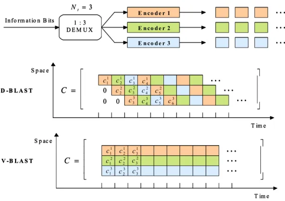
Spatial multiplexing (SM) is a technique that yields an increased bit rate by using multiple antennas at both end of the wireless link [1]-[3]. This increase comes at no extra bandwidth and power consumption. However, such a technique calls for an efficient way to map the transmit signals to individual antenna elements. At the receiver, the individual data streams are separated and demultiplexed to yield the original transmitted signals, as illustrated in Figure 2.2. The separation is made possible by the fact that the rich multipath contributes to lower correlation between MIMO channel coefficients, and hence creates a desirable coefficient matrix condition (i.e., full rank and low condition number) to resolve Nt unknowns from a linear system of Nr equations. In the following, we will introduce two SM schemes: D-BLAST and V-BLAST.

2.2.1 Diagonal Bell Labs’ Layered Space-Time

The Layered Space-Time processing concept was first introduced by Foschini [1] at Bell Labs. The first version, D-BLAST, utilizes multiple antenna arrays at both the transmitter and receiver, and an elegant diagonally-layered coding structure in which code blocks are dispersed across diagonals in space-time. The encoding and decoding procedures are described as follows:

• Encoding:

Considering a system equipped with Nt transmit and Nr receive antennas, the encoder applies the space-time codes to the input to generate a semi-infinite matrix C of Nt rows to be transmitted. Figure 2.5 shows the encoding scheme, where cτk,

representing an element in the kth row and τ column of C, is transmitted by the kth th

transmit antenna at time τ . The data received at time τ by the lth receive antenna is

l

r_τ , which contains a superposition of _ck

τ , 1, 2, ,k = … Nt , and an AWGN noise

component. Each subsequence is encoded using a conventional 1-D constituent code with low decoding complexity.

• Decoding:

At any instance τ , the received datum vector is r_τ =H c_{τ τ} +η (refer to Section _τ

2.1). The decoding task is to determine c c1_{, ,...,}2 cNt T

τ =  τ τ τ 

c with the only available information being r and τ H . The D-BLAST uses a repeated process of interference τ suppression, symbol detection and interference cancellation for decoding all symbols,

1 1 , ,...,

t t

N N

c_τ c_τ − c_{τ. Such decoding process could be expressed in a general form:}

Let the QR decomposition of Hτ be Q Rτ τ, where Qτ is an Nr×Nr unitary matrix and R_τ is an Nr×Nt upper triangular matrix. We modify the received data to get

Nr H H H H H τ τ τ τ τ τ τ τ τ τ τ τ τ τ τ τ τ τ = = + = + = + I η y Q r Q H c Q η Q Q R c Q η R c η (2.8) where 1, 1,1 1,2 2, 2,2 1 1 2 2 , 0 0 0 , , 0 0 0 0 0 0 0 0 t t t t r r N N N N N N r r r r r y y r y τ τ τ τ τ τ τ τ τ τ τ τ τ τ τ η η η         _{ }     _{ }       = =_{ } =   _{ }     _{ }         _{ }         y R η (2.9)

Since R_τ is upper triangular,

_yk _{r c}k k k, k

Now, we can figure out that the interference from _{c ,} l

t

l k< ≤N , are first suppressed in _{y and the residual interference terms in Equation 2.10 can be cancelled by the} k

available decisions _cˆk 1

τ+ ,cˆτk+2,…, ˆcτNt. Assuming all these decisions are correct, the present decision variable is

k k k k, k_{, 1, 2, ,} t

cτ =r cτ τ +ητ k= … N (2.11)

The relationship between _{c and} k _{c in Equation 2.11 can be interpreted as the input} k

and output of a SISO channel with the channel power gain _rk k, 2 _{and AWGN. The} channel power gain _rk k, 2 _{are independently chi-squared distributed with 2×(N}

r−k+1) degrees of freedom. Moreover, if there are no decision feedback errors, we can treat the

kth row of the C matrix as transmitted over a (Nt, Nr)=(1, Nr−k+1) system without interference from the other rows and all fades are i.i.d.

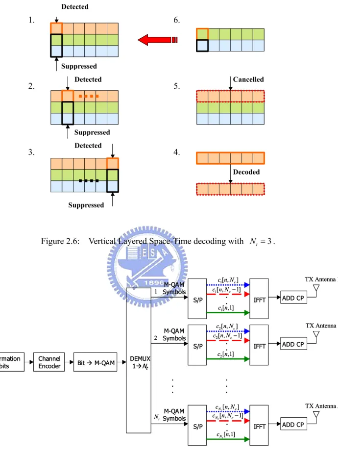
Figure 2.6 shows typical decoding steps (suppression, detection, decoding and cancellation) performed in a D-BLAST system. The receiver generates decisions for the first diagonal of C, 1 1 ˆ , c 2 2 ˆ ,... c ,ˆ t t N N

c . Based on these decisions, the diagonal is decoded and fed back to remove the contribution of this diagonal from the received data. The receiver continues to decode the next diagonal and so on. The encoded substreams share a balanced presence over all paths to the receiver, so none of the individual substreams is subject to the worst path.

2.2.2 Vertical Bell Labs’ Layered Space-Time

The diagonal approach suffers from certain implementation complexities that make it inappropriate for initial implementation. Therefore, Foschini proposed another low-complexity version of detecting the symbols transmitted synchronously over

antennas, that is, V-BLAST [3]. The “V” here stands for the vertical vector mapping process, which differs from the diagonal form in D-BLAST. In V-BLAST, no inter-substream coding, or coding of any kind, is required, though conventional coding of the individual substreams may certainly be applied. In [4], a vertical-and-horizontal coding structure along with iterative detection and decoding (IDD) was promoted and showed to significantly improve the performance with limited complexity.

Figures 2.5 and 2.7 displays the typical encoding and decoding steps in V-BLAST. The decoding process can also be interpreted via the general form (QR decomposition) as mentioned in decoding D-BLAST. In each step I, the signals from all but one transmit antenna are eliminated using interference suppression and cancellation with already detected signals. Following the data model in D-BLAST, at a given time instant τ , let i 1 τ = ₌ H H and i 1 τ = ₌

r r at the first decoding step. In each step i, the nulling

matrix _{G is calculated as the pseudo-inverse of} i _H i

(

)

1 ( ) ( ) ( ) i i i H i i H + − = = G H H H H (2.12)

Each row of _{G can be used to null all but the ith desired signal. Instead of choosing} i

an arbitrary layer to be detected first, it was suggested to start with the layer showing the biggest post-detection SNR to efficiently reduce the error propagation effect [3]. This corresponds to choosing the row of _{G with the minimum norm and defining the} i

corresponding row, T_i k

w , as the nulling vector at this step:

{1 1} 2 ,..., arg min || ( ) || i i i j j k k k − ∉ = G (2.13) _i ( i T)_i k = k w G (2.14)

transmitted from antenna k and we get a soft decision value _i i i k T i k c_τ = w r (2.15) _τ

Now the k th layer can be detected within the constellation set S that we use: _i

_ˆ ki _{arg min ||} ki _||2

x S

cτ c cτ

∈

= − (2.16)

As soon as one layer is detected, we can improve the detection performance for the subsequent layers by subtracting the part of the detected signal from the received vector, _i 1 _{i ˆ ki}

( )

_i ki c τ+ = −τ τ r r H (2.17) where

( )

_i ki

H denotes the kith column of H . After canceling out the signal from the i

kith transmit antenna, the channel matrix is reduced to

( )

1 ki

i+ ₌ i

H H (2.18)

where the notation

( )

_i ki

H denotes the matrix obtained by zeroing columns k k₁, ,...,₂ k _i

of _{H . Since we decrease the number of layers to be nulled out in the next step by} i

one, the diversity gain is increased by one at each step (from (Nr−Nt+i) to (Nr−Nt+i+1)). This can be proven by the Cauchy-Schwartz inequality [3]. The full Zero-Forcing V-BLAST detection algorithm can be summarized as follows:

Initialization: 1 i←

( )

1₌ 1 + G H 1 2 1 arg min || (_j ) ||j k = G Recursion:

( ) i i i T k = k w G i i k T i k c = w r ˆki ( ki)

c =Q c , Q(⋅) denotes the slicing operation 1 _{ˆ ( )}ki ki i+ _{= −}i _c i r r H

( )

1 ki i+ ₌ i H H

( )

i+1₌ i+1 + G H {1 } 1 2 1 arg min || (_, ) || i i i _{j k k} j k₊ + ∉ = G 1 i← +i

The post-processing SNR for the kith detected component of c is

2 2 2 | | || || i i i k k k c ρ σ < > = w (2.19)

where the expectation value in the numerator is taken over the constellation set S. Another way to improve detection performance especially for mid-range SNR values is to replace the ZF nulling matrix by the more powerful MMSE one [3]:

1 1 ( ) ( ) i i H i i H SNR −   =_ + _   G H H I H (2.20)

In this case, in additional to nulling out the interference, the noise level on the channel is taken into account. Thus, the SNR has to be estimated at the receiver. Figure 2.7 shows the typical decoding procedure in V-BLAST.

The D-BLAST code blocks are organized along diagonals in space-time. It is this coding that leads to D-BLAST’s higher spectral efficiencies for a given number of transmit and receive antennas.

2.3 Review of OFDM

OFDM can be regarded as either a modulation or a multiplexing technique. The basic concept of OFDM is to split a high rate data stream into a number of lower rate streams that are transmitted simultaneously over subcarriers. In order to eliminate the effect of inter-symbol interference (ISI), a guard time is appended to each OFDM symbol. The guard time is chosen to be larger than the maximum delay spread such that the current OFDM symbol never hears the interference from the previous one. However, this method will cause the inter-carrier interference (ICI) due to the loss of orthogonality between subcarriers. To solve this problem, OFDM symbols are cyclically extended in the guard time to introduce cyclic prefix (CP). This ensures that the delayed replicas of an OFDM symbol always have an integer number of cycles within the FFT interval. As a result, CP resolves both ISI and ICI problems caused by multipath, as long as the delay spread of channel is smaller than the length of CP. Besides, adding CP makes the transmitted OFDM symbol appear periodic, and the linear convolution process of the transmitted OFDM symbols (containing CP) with channel impulse response will be translated into a circular convolution one. According to discrete-time linear system theory, this circular convolution is equivalent to multiplying the frequency response of the OFDM symbol with the channel’s frequency response. This property can be demonstrated as follows:

Assuming that the channel length is smaller than Ncp (number of samples in CP), we can express the received datum vector y as

1 0 1 1 1 0 1 0 1 0 0 0 1 0 0 0 0 0 0 0 0 0 c cp c c cp cp cp N N N N N N N x h h h y h h h x x y h h h x η η − − − − −             _{ }      _{=  +}      _{ }           _{  }           y η H x (2.21)

When we use SVD, we have

_{H FΛM (2.22) =} H

where _FFH _{=I and MM}H _{=I . If we let x MX= and Y F y , then we can get =} H

( ) H H H H = = + = + = + F η Y F y F Hx η F HMX N ΛX N (2.23)

It is interesting to note that when the guard period contains a CP, that is, x_−i =x_{N i−} for 1,..., _cp

i= N , Equation 2.21 can be rewritten in a more compact matrix form

0 1 0 1 1 1 1 0 1 0 _{0 1} 0 0 1 0 0 0 0 0 0 0 0 0 0 0 cp cp c c c cp cp cp cp N N N N N N N N N h h h h h h y x h h h y h h h x h h h η η − − − −           _{ }     _{= }  ₊    _{ }      _{ }                    (2.24)

And H becomes the so called “circulant matrix” and has the property that _{H Q ΛQ=} H _,

where Q is a DFT matrix with klth entry as

1 2 c kl j N kl c e N π − = Q (2.25)

And the transformed symbol is _{x Q X=} H _{(IDFT of x). Thus X can be interpreted as}

symbols in the frequency domain. At the receiver, we have the received data y being transformed to Y

( ) H H H H H = = + = + = + N Λ Y Q y Q Hx η Q HQ X Q η ΛX N (2.26)

Now, we can realize that by using CP, the OFDM modulation is equivalent to multiplying the frequency domain signals of the OFDM symbol (that is, X) with the channel’s frequency responseΛ .

Broadband transmission over multipath channels usually exhibits frequency selective fading. Since data rate requirements can be expected to increase even further in the future, this effect is likely to amplify. In OFDM, frequency diversity can be realized through coding and interleaving across subcarriers. Because information bits are separated over many subcarriers, the impairment of fading occurring at particular frequency tones can be mitigated. As a consequence, in the coded OFDM systems the presence of frequency selective fading actually saves the frequency tones at fading. Depending on the coding rate and interleaving death, gains can be achieved at locations experiencing significant delay spread.

It can be concluded that OFDM is a powerful modulation technique that increases bandwidth efficiency and simplifies the removal of distortion due to a multipath channel. Advances in fast Fourier transform (FFT) algorithm enable OFDM to be efficiently implemented in hardware, even for a large number of subcarriers. The key advantages of OFDM transmission are summarized as follows:

1. OFDM deals with multipath delay channels in an efficient way. The implementation complexity is significantly lower than that of a single carrier system with an equalizer.

2. OFDM has a long symbol period (compared to an equal data-rate single-carrier system) that allows OFDM to be more robust against impulse noise.

different modulation modes depending on the channel characteristic or the noise level. Therefore, improved performance can be achieved in this systematic way.

2.4 V-BLAST

Based

OFDM

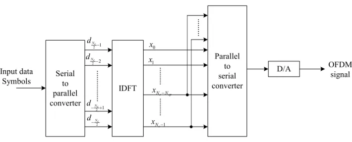
Due to the scarcity of radio spectrum, high spectral efficiency becomes a must-have requirement that encourages modern wireless modems toward this trend. An evolution of the V-BLAST supporting OFDM modulation seems to be a solution that can dramatically increase the capacity of wireless radio links with no additional power and bandwidth consumption. The core idea in such scheme is that with the aid of OFDM, the whole detection problem in MIMO-OFDM would be translated into Nc parallel sub-problems.

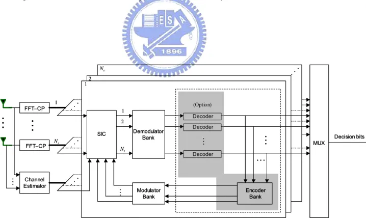
In the transmitter, as shown in Figure 2.8, a traditional 1-D channel encoder is used to encode the information bits. These coded bits are then mapped on the symbols of constellation adopted for each subcarrier. At a given time slot n, N_c×N_t bit streams{ [ , ]:c n k k_i =0,1,…N_c} for i=1, 2 ,… N_t are fed to the IFFT at the ith transmit antenna on the kth subcarrier to generate the nth transmitted OFDM symbols from the

ith transmit antenna.

At the receiver side, as shown in Figure 2.9, receive antennas 1~Nr will receive the radiate signal from transmit antennas 1~Nt, where the V-BLAST requires Nr≥ Nt to ensure its proper working. The received data at each receive antenna will then pass through a FFT with the removal of the CP. The FFT output, at the receive antenna j, is a set of Nc signals, one for each frequency subcarrier, expressed as

_, 1 [ , ] Nt [ , ] [ , ] [ , ] 1, 2,..., j j i i j c i r n k H n k c n k η n k k N = =

∑

+ ∀ = (2.27)

transmit antenna i to the receive antenna j at frequency k, and [ , ]η_j n k denotes the additive complex Gaussian noise at the receiver antenna j and frequency k with two-sided power spectral density N₀/ 2 per dimension and uncorrelated for different

n’s, k’s, and j’s.

2.5 MIMO Beamforming: Concept and

Technique

Traditionally, the intelligence of the multiantenna system is located in the weight selection algorithm. Simple linear combining can offer a more reliable communications link in the presence of adverse propagation conditions such as multipath fading and interference. Beamforming is a key technique in smart antenna and increases the average SNR. In the following, we will introduce two schemes: beamforming and eigenbeamforming.

2.5.1 Generic Beamforming

As a feedback channel from the receiver to the transmitter can be obtained, beamforming can be utilized to maximize the receiver SNR and provide array gain [42]. With beamforming technique applied to both the transmitter and receiver, the beamformer output of the receiver is given by

ˆ H

(

)

H H

T T

R R R

s =w Hw s+n =w Hw s +w n (2.39)

where w_R and w_T denote the weight vectors of transmitter and receiver, respectively,

illustrated by Figure 2.10. If w_R and w_T are chosen as the dominant left and right singular vectors associated with the channel matrix H, the beamformer output can be rewritten as

1 2 * 1

ˆ _R

s =λ s+ w n (2.40)

where λ₁ is the largest eigenvalue of the matrix HHH_{. According to Equation 2.40, the}

corresponding SNR is SNR_BF T_{2 1} n P λ σ = (2.41)

where P_T is the total transmitted power.

2.5.1 Eigenbeamforming Technique

The eigenbeamforming is an attractive method for downlink [43]. It can provide good diversity gains with less amount of feedbacks due to the short-term selection of eigenmode. Eigenbeamforming is particularly suitable for spatially correlation channels, and is easily applied to the spatial downlink channel. This is because that the spatial downlink channel possesses a higher spatial correlation and few dominant eigenmodes, in which each eigenmode can be considered as an uncorrelated path to the mobile station [44]. In a cellular system, the signal can be spatially selectively transmitted with only few directions due to the vanish of local scatters around the antenna array of the base station. This makes the eigenbeamforming effectively. Consider a system with M_T transmit antennas at the base station and M_R receive antennas at the mobile station. The received signal vector at the mobile station is given by

y( )t = γH( ) ( ) ( )t w t s t +n( )t (2.42) where γ is the input SNR, H(t) is the channel matrix, and w(t) is the beamforming

weight vector. Assume that beamforming vector is normalized to one, i.e., w( )t 2 =1. The instantaneous SNR at the receiver is written as

H( ) H( ) ( ) ( )

rec t t t t

γ = wγ H H w (2.43)

This suggests that the optimal weight vector, maximizing the instantaneous SNR, can be obtained as follows: ( ) ( ) 2 ₁ arg max H( ) ( ) opt t = _{w =} t H t t w w R w (2.44) where ( )_{t =} H( ) ( )_{t t} H

R H H . The corresponding solution is the dominant eigenvector associated with the largest eigenvalue of the matrix R_H(t). Note that since the channel information must be sent to the base station, this method is called close-loop beamforming. Suppose that the instantaneous channel matrix is not available. Assume that the beamforming vector is time-invariant (or very slowly varying). The beamforming vector can be obtained by maximizing the mean SNR as follows:

[

]

2 2 1 1 arg max ( ) arg max ms rec H E γ t ≤ ≤ = = w H w w w R w (2.45)

where R_H =E_R_H( )t _ . The beamforming that uses w_ms is called the blind beamforming that can be employed in CDMA system with lower mobile speed.

2.6 Computer Simulations

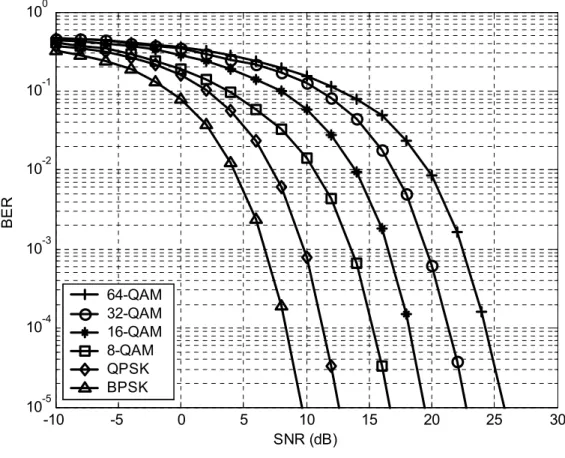
In this section, we simulate the V-BLAST performance both for the ideal and realistic case. We define the relation between SNR and E N at each receive _{b 0}

antenna as follows:

(

)

0 0 0 signal power SNR 1 noise power s b t s s b t s E E N M T T E N M N B _N N T ⋅ ⋅ = = = = ⋅ ⋅ (2.46)

where E is the symbol energy, _s T is the symbol duration, B is the system bandwidth _s

and M is the modulation order. Throughout the following simulations, the system transmit power is normalized to 1, and hence the noise power corresponding to a specific E N is generated by _{b 0 noise power} 0 b t N E N M = ⋅ ⋅ (2.47)

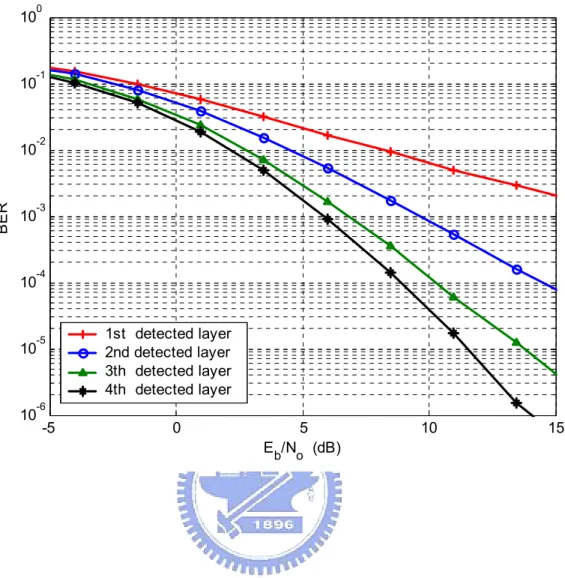
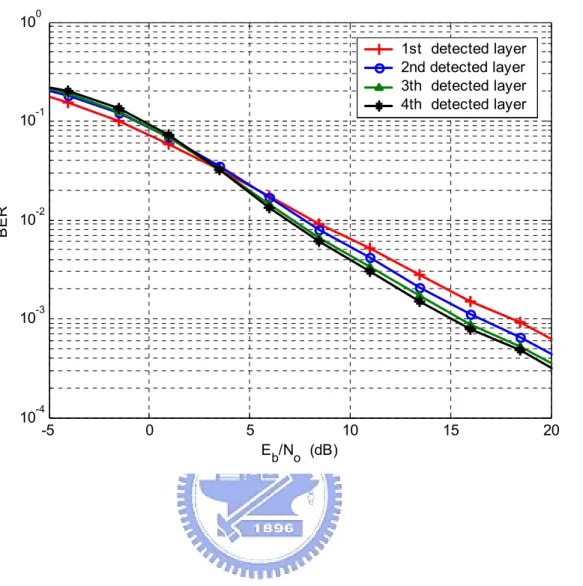
Figure 2.10 shows the BER performance of the (Nt, Nr) = (4, 4) ZF V-BLAST system with ideal detection and cancellation. It is obvious that in the ideal case, the diversity gain increases as the number of effective transmit antennas decreases. However, as shown in Figure 2.11, the realistic V-BLAST system suffers from error propagation and hence the diversity gain degrades. In Figure 2.12, we compare two equal rate V-BLAST systems. It is interesting to see that the system with fewer transmit antennas will outperform the one with more transmit antennas in the BER performance. This phenomenon hints that given a MIMO channel and some transmit power budget, we can improve the MIMO system performance by simply adjusting transmission parameters at no cost of transmission rate. So, it strongly motivates us involve the concept of adaptive modulation in MIMO, which will be described in Chapter 3.

Figure 2.1: Diagram of a MIMO wireless transmission system.

Figure 2.2: An illustration of a spatial multiplexing system.

Transmitter Receiver -antennas Rich Scattering Environment T N NR -antennas 1,1 t

h

2,1 t

h

1,N_t t

h

, r t N N t

h

#

#

⊕

⊕

⊕

1 t

η

2 t

η

2 t

η

1 t

s

2 t

s

t N t

s

1 t

r

2 t

r

r N t

r

Transmitter Receiver -antennas Rich Scattering Environment T N NR -antennas 1,1 t

h

2,1 t

h

1,N_t t

h

, r t N N t

h

#

#

⊕

⊕

⊕

1 t

η

2 t

η

2 t

η

1 t

s

2 t

s

t N t

s

1 t

r

2 t

r

r N t

r

Transmitter Receiver

"

"

"

T im e S p ac e 1 : 3 D E M U X In fo rm at io n B its E n co d e r 1 E n co d e r 2 E n co d e r 3

"

"

"

1 1 c 2 2 c 3 3 c 1 2 c 2 3 c 3 4 c 1 3 c 2 4 c 3 5 c 1 4 c 2 5 c 3 6 c 3 t N =             C = 0 0 0

"

"

"

T im e S p ac e 1 1 c 2 1 c 3 1 c 1 2 c 2 2 c 3 2 c 1 3 c 2 3 c 3 3 c             C = D -B L A S T V -B L A S T

"

"

"

T im e S p ac e 1 : 3 D E M U X In fo rm at io n B its E n co d e r 1 E n co d e r 2 E n co d e r 3

"

"

"

1 1 c 2 2 c 3 3 c 1 2 c 2 3 c 3 4 c 1 3 c 2 4 c 3 5 c 1 4 c 2 5 c 3 6 c 3 t N =             C = 0 0 0

"

"

"

T im e S p ac e 1 1 c 2 1 c 3 1 c 1 2 c 2 2 c 3 2 c 1 3 c 2 3 c 3 3 c             C = D -B L A S T V -B L A S T

Figure 2.4: Diagonal and Vertical Layered Space-Time encoding with N_t = . 3

Figure 2.5: Diagonal Layered Space-Time decoding with N_t = . 3

Decoded Cancelled Suppressed Suppressed Detected Detected Detected Detected 1. 2. 3. 4. 5. 6.

Figure 2.6: Vertical Layered Space-Time decoding with N_t = . 3

Figure 2.7: V-BLAST based MIMO-OFDM transmitter architecture.

Suppressed Suppressed Detected Detected Decoded Suppressed Detected Cancelled 1. 2. 3. 4. 5. 6. . . TX Antenna Nt TX Antenna 2 TX Antenna 1 ADD CP S/P IFFT S/P IFFT ADD CP S/P IFFT ADD CP . . . . . Information

bits ChannelEncoder Bit Æ M-QAM DEMUX1ÆNt

1[ , c] c n N 1[ , c 1] c n N − 1[ ,1] c n 2[ ,1] c n 2[ , c 1] c n N − 2[ , c] c n N . . [ ,1] t N c n [ , ] t N c c n N [ , 1] t N c c n N − 1 2 t N . . . M-QAM Symbols M-QAM Symbols M-QAM Symbols . . TX Antenna Nt TX Antenna 2 TX Antenna 1 ADD CP S/P IFFT S/P IFFT ADD CP S/P IFFT ADD CP . . . . . Information

bits ChannelEncoder Bit Æ M-QAM DEMUX1ÆNt

1[ , c] c n N 1[ , c 1] c n N − 1[ ,1] c n 2[ ,1] c n 2[ , c 1] c n N − 2[ , c] c n N . . [ ,1] t N c n [ , ] t N c c n N [ , 1] t N c c n N − 1 2 t N . . . M-QAM Symbols M-QAM Symbols M-QAM Symbols

Figure 2.8: V-BLAST based MIMO-OFDM receiver architecture. . . . . . RX Antenna Nr RX Antenna 2 RX Antenna 1 Remove CP FFT FFT FFT . . . . . . . . V-BLAST MUX 1 2 c N [ ,1] r N r n [ , ] r N c r n N [ , 2] r N r n . . 2[ ,1] r n 2[ , c] r n N 2[ , 2] r n . . 1[ ,1] r n 1[ , c] r n N 1[ , 2] r n • • • . . . . . . 1 ˆ [ , c] c n N M-QAMÆBits Remove CP Remove CP Channel Decoder 2 ˆ [ , _c] c n N ˆ [ , ] t N c c n N 1 ˆ [ , 2] c n 2 ˆ [ , 2] c n ˆ [ , 2] t N c n . . . 1 ˆ [ ,1] c n 2 ˆ [ ,1] c n ˆ [ ,1] t N c n . . . . . RX Antenna Nr RX Antenna 2 RX Antenna 1 Remove CP FFT FFT FFT . . . . . . . . V-BLAST MUX 1 2 c N [ ,1] r N r n [ , ] r N c r n N [ , 2] r N r n . . 2[ ,1] r n 2[ , c] r n N 2[ , 2] r n . . 1[ ,1] r n 1[ , c] r n N 1[ , 2] r n • • • • • • . . . . . . 1 ˆ [ , c] c n N M-QAMÆBits Remove CP Remove CP Channel Decoder 2 ˆ [ , _c] c n N ˆ [ , ] t N c c n N 1 ˆ [ , 2] c n 2 ˆ [ , 2] c n ˆ [ , 2] t N c n . . . 1 ˆ [ ,1] c n 2 ˆ [ ,1] c n ˆ [ ,1] t N c n

-5 0 5 10 15 10-6 10-5 10-4 10-3 10-2 10-1 100 E_b/N_o (dB) BER 1st detected layer 2nd detected layer 3th detected layer 4th detected layer

Figure 2.10: ZF V-BLAST performance with ideal detection and cancellation. QPSK modulation is used. (Nt, Nr) = (4, 4).

-5 0 5 10 15 20 10-4 10-3 10-2 10-1 100 E_b/N_o (dB) BE R 1st detected layer 2nd detected layer 3th detected layer 4th detected layer

Figure 2.11: ZF V-BLAST performance with error propagation. (Nt, Nr ) = (4, 4). QPSK modulation is used.

-5 0 5 10 15 20 25 10-5 10-4 10-3 10-2 10-1 100 (4Tx, 4Rx) QPSK (2Tx, 4Rx) 16-QAM E_b/N_o (dB) BER

Figure 2.12: Comparison of ZF V-BLAST (Nt, Nr) = (4, 4) with QPSK modulation and (Nt, Nr) = (2, 4) with 16-QAM modulation.

Chapter 3

Adaptive Modulation Assisted

MIMO-OFDM Systems

The combined application of MIMO and OFDM (MIMO-OFDM) yields a noticeable physical layer capable of meeting the requirements for 4G broadband wireless systems [17]. Thanks to OFDM, which is characterized by possessing multi-channels over frequencies, the signal processing techniques involved in MIMO-OFDM could be borrowed from the sophisticated space-time ones by admitting the virtual equivalence between time and frequency in some particular scenarios.

From the analysis of MIMO channel capacity, we figure out that the waterfilling distribution of power over channels with different SNR values achieves the optimal transmission scheme [34]. However, while the waterfilling distribution will indeed yield the optimal solution, it is difficult to compute, and also assumes infinite granularity in the constellation size, which is not practically realizable.

In this chapter, we introduce a practical adaptive loading procedure for MIMO-OFDM that uses the V-BLAST as both its channel quality indicator and detection algorithm. Bit and power are allocated in a manner to fix the total transmission power while maximizing the data rate and yet still maintaining a target system performance.

3.1 Adaptive

Modulation

Wireless communication channels typically exhibit time-variant quality fluctuations and hence conventional fixed-mode modems usually suffer from bursts of error (see Figure 3.4 to get the idea). This defect could be somewhat mitigated if the system was designed to provide a high link margin, that is, determine transmission parameters based on the worst-case channel conditions to render the immunity against channel impairments. However, it results in insufficient utilization of the full channel capacity. An efficient approach of avoiding these detrimental effects is to dynamically adjust transmission parameters based on the near instantaneous channel quality information. In general, the following steps have to be taken to react to the change in channel condition for an adaptive wireless transceiver.

1. Channel quality estimation: If the communication between the two stations is bi-directional and the channel can be considered reciprocal, then each station can estimate the channel quality on the basis of received symbols, and adapt the parameters of the local transmitter to this estimation in an open-loop manner. 2. Choice of the appropriate parameters for the next transmission: The transmitter

has to select the appropriate modulation mode for each sub-channel based on the prediction of the channel quality for the next timeslot.

3. Signaling of the employed parameters: The receiver has to be informed, as to which demodulator parameters to employ for the received packet. This information can be either conveyed by the transmitted signal itself, at the cost of a loss of effective data throughput, or estimated by a blind detection mechanism at the receiver.