流體介質中的粒子通訊:相加性反高斯雜訊的通道容量界線

國

立

交

通

大

學

電信工程研究所

碩

士

論

文

流體介質中的粒子通訊:相加性反高斯雜訊的通道容量界線

Molecular Communication in Fluid Media: Bounds on the Capacity of the

Additive Inverse Gaussian Noise Channel

研 究 生：張惠婷

指導教授：莫詩台方 教授

Molecular Communication in Fluid Media: Bounds on the Capacity of the

Additive Inverse Gaussian Noise Channel

研 究 生：張惠婷

Student：Hui-Ting Chang

指導教授：莫詩台方 教授

Advisor：Prof. Stefan M. Moser

國 立 交 通 大 學

電 信 工 程 學 系 碩 士 班

碩 士 論 文

A Thesis

Submitted to Institute of Communication Engineering

College of Electrical Engineering and Computer Science

National Chiao Tung University

in partial Fulfillment of the Requirements

for the Degree of

Master of Science

in

Communication Enginering

March 2013

Hsinchu, Taiwan, Republic of China

Information Theory

Laboratory

Dept. of Electrical and Computer Engineering National Chiao Tung University

Master Thesis

Molecular Communication in

Fluid Media: Bounds on the

Capacity of the Additive Inverse

Gaussian Noise Channel

Chang Hui-Ting

Advisor: Prof. Dr. Stefan M. Moser

National Chiao Tung University, Taiwan Graduation Prof. Dr. Yu Ted Su

Committee: National Chiao Tung University, Taiwan Prof. Dr. Scott Ch. Huang

相加性反高斯雜訊的通道容量界線

研究生：張惠婷

指導教授：莫詩台方 教授

國立交通大學電信工程研究所碩士班

中文摘要

在本篇論文中，我們研究一個相當新且近代的通道模型，該通道利用

常速流體當中的化學粒子交換來做為溝通的訊息。這些粒子由傳送端出發

至接收端的路徑，我們將其視為一維空間來做模擬。很典型的通訊應用像

是我們將奈米級的儀器置入血管中，以完成傳遞訊息的任務。在這個情況

下，我們不再依賴電磁波傳遞訊息，而是將訊息放在釋放粒子的時間點上。

一旦粒子被傳送端釋放進入流體中時，會在介質中行布朗運動，這將會對

粒子到達接收端的時間產生不確定性，這樣的不確定性就是我們的雜訊。

我們用反高斯分布來描述這樣的雜訊。此篇研究將重點放在相加性雜訊通

道以描述基本的通道容量趨勢。

我們深入研究此模型，並分析出新的通道容量上界與下界。 這些界線

是漸進緊的，也就是說，如果平均延遲的限制可放寬至無限大，或是介質

流體流速趨近無限大，則相對應的漸進通道容量可被精確的推導出來。

Abstract

Molecular Communication in Fluid Media:

Bounds on the Capacity of the Additive

Inverse Gaussian Noise Channel

Student: Chang Hui-Ting Advisor: Prof. Stefan M. Moser

Institute of Communication Engineering National Chiao Tung University

In this thesis a very recent and new channel model is investigated that describes communication based on the exchange of chemical molecules in a liquid medium with constant drift. They travel from the transmitter to the receiver at two ends of a one-dimensional axis. A typical application of such communication are nano-devices inside a blood vessel communicating with each other. In this case, we no longer transmit our signal via electromegnetic waves, but we put our information on the emission time of the molecules. Once a molecule is emitted in the fluid medium, it will be affected by Brownian motion, which causes uncertainty of the molecule’s arrival time at the receiver. We characterize this noise with an inverse Gaussian distribution. Here we focus solely on an additive noise channel to describe the fundamental channel capacity behavior.

This new model is investigated and new analytical upper and lower bounds on the capacity are presented. The bounds are asymptotically tight, i.e., if the average-delay constraint is loosened to infinity or if the drift velocity of the liquid medium tends to infinity, the corresponding asymptotic capacities are derived precisely.

Never in my life did I realize that learning could be so enjoyable, until I started my first lesson with Prof. Stefan M. Moser. in 2008. I was so much encouraged to ask questions and discuss our ideas during his wonderful classes. Great thanks to his kind acceptance for me as a member of Information Theory Laboratory (IT Lab), NCTU. Under his patient guidance, I had my happiest research period. He always pays fully attention on my meeting presentation and gave very useful suggestions for improvement.

He always shows warm welcome whenever I knock his office door for questions or even advice of life. Moreover, I cherish the moments when we sat down together at his place with his wife Yin-Tia and son Matthias. There, we shared about life, educations, coffee, trips and all sorts of thing. These are the moments which lighten my thoughts deeply. I would never live my life as faithfully and clearly like now without the help from them. To me, he is my Prof. Albus Dumbledore. Thank you for giving me so many wonderful lessons.

Big thanks to Yuan-Chu. She is a strong support and a very nice accompany during my time in NCTU. Without her, this thesis wouldn’t be complete.

Thanks to Gu-Rong Lin’s advice during my master study. He is a very helpful former lab member who has a very kind heart. Thanks to Hsuan-Ying Lin, who is always patient for my questions and has helped me a lot.

At the end but not the least, thanks to the financial support of my parents. Without them, it would be more difficult to finish my master study.

Flight back to Taiwan, 18 March 2013

Contents

Acknowledgments III

List of Figures VI

1 Introduction 1

1.1 General Molecular Communication Channel Model . . . 1

1.2 Mathematical Model . . . 2

1.3 Capacity . . . 4

2 Mathematical Preliminaries 5 2.1 Properties of the Inverse Gaussian Distribution . . . 5

2.2 Power Inverse Gaussian and Its Properties . . . 10

2.3 Related Lemmas and Propositions . . . 11

3 Known Bounds to the Capacity of the AIGN Channel 13 4 Our Different Trials of Lower Bounds 16 4.1 Lower Bounds of h(Y ) Based on h(X) . . . 16

4.2 Capacity Lower Bounds Based on Theorem 4.1 . . . 18

4.2.1 Lower Bound 1: Taylor Expansion . . . 18

4.2.2 Lower Bound 2 . . . 20

4.3 Lower Bound Based on the Convolution of Exponential and Inverse Gaussian Distribution . . . 22

5 Our Different Trials of Upper Bounds 27 5.1 Exponential Distribution as Output Distribution . . . 27

5.2 Inverse Gaussian Distribution as Output Distribution . . . 28

5.3 PIG Distribution as Output Distribution . . . 32

5.4 Shifted Gamma Distribution as Output Distribution . . . 35

6 Asymptotic Capacity of AIGN Channel 37 6.1 When v Large . . . 37

7 Discussion and Conclusion 41

List of Figures

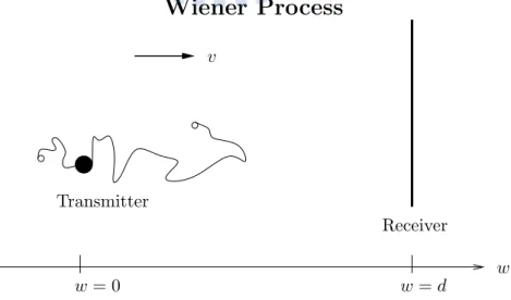
1.1 Wiener process of molecular communication channel. . . 1

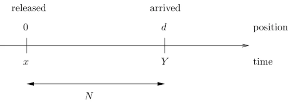
1.2 The relation between the molecule’s time and position. . . 2

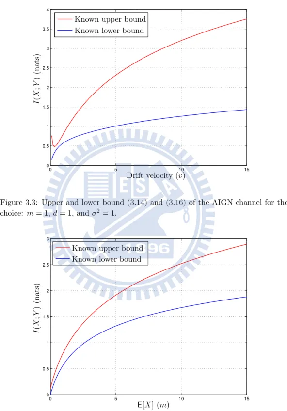
3.3 Upper and lower bound (3.14) and (3.16) of the AIGN channel for the choice: m = 1, d = 1, and σ2 = 1. . . 15

3.4 Upper and lower bound in (3.14) and (3.16) of the AIGN channel for the choice: v = 1, d = 1, and σ2 _{= 1. . . . 15}

4.5 m = 2, σ2 = 1, d = 1 . . . 20 4.6 m = 2, σ2 = 1, d = 1 . . . 22 4.7 m = 2, σ2 _{= 1, d = 1 . . . . 25} 4.8 v = 2, σ2= 1, d = 1 . . . 25 5.9 m = 2, σ2 = 1, d = 1 . . . 31 5.10 v = 2, σ2_{= 1, d = 1 . . . . 31} 5.11 m = 2, σ2 = 1, d = 1 . . . 34 5.12 v = 2, σ2= 1, d = 1 . . . 34 5.13 m = 2, σ2 _{= 1, d = 1 . . . . 36}

6.14 Setting parameter: m = 2, d = 1 and σ2 = 1. . . 38

Introduction

1.1

General Molecular Communication Channel Model

Usually, we transmit our signal with electromagnetic waves in the air or in wires. Recently, people are more and more interested in communication within nanoscale networks. But when we want to transmit our signal via these tiny devices, we face some problems that the antenna size of them are restricted and the energy that could be stored in them is very little. Therefore, we solve these problems with providing a different type of communication instead. This thesis focuses on a channel which operates in a fluid medium with a constant drift velocity. The transmitter is a point source with many molecules to be emitted. The receiver waits on the other side for the molecules’ arrival. The information is encoded in the emission time of the molecules, X, which takes value in a finite set. One application example is blood vessel, which has a blood drift. The nanoscale device could be any medical inspection device that is inserted in our body.

Wiener Process

Chapter 1 Introduction

Once the nanoscale molecules are emitted in the fluid medium, they are effected by Brownian motion which causes uncertainty of the arrival time at the receiver. We describe this type of channel noise with an inverse Gaussian distribution. Now, consider a channel as shown in Figure 1.1 where w is the position parameter, d is the receiver’s position on w axis and v is the drift velocity, v > 0. The transmitter is placed at the origin of w axis. It emits a molecule into a fluid with positive drift velocity, v. The information is put on the releasing time. In order to know this

information, the receiver ideally subtracts the average traveling time, d_v, from the

arrival time. Note that once a molecule arrives at the receiver, it is absorbed and never returns to the fluid. Moreover, every molecule is independent of each other.

This molecular communication channel model was proposed by Srinivas, Adve and Eckford [1].

1.2

Mathematical Model

Let W (x) be the position of a molecule at time x that travels via a Brownian

motion medium. Let 0≤ x1 < x2<· · · < xk be a sequence of time indices ordered

from small to large. Then, W (x) is a Wiener process if the position increment

Ri = W (xi−1)− W (xi) are independent random variables with

Ri∼ N!v(xi− xi−1), σ2(xi− xi−1)" (1.1)

where σ2 ₌ D

2 with D being the diffusion coefficient, which depends on the

tem-perature and the stickiness of the fluid and the size of the particles. Assuming the

molecule is released at time x = 0 at position W (0) = 0, the position at time ˜x is

W (˜x)_{∼ N}!v˜x, σ2_{x". The probability density function (PDF) of W is given by:˜}

fW(w; ˜x) = 1 √ 2πσ2_x˜exp # −(w− v˜x) 2 2σ2_x˜ $ . (1.2)

In our communication system, instead of looking at the position of the molecule at a certain time, we turn our focus on its arriving time at the receiver for a fixed distance d. x Y released arrived N time 0 d position

We release the molecule at time x from the origin, W (x) = 0 and x_{≥ 0.} Assum-ing that after travelAssum-ing for a random time N , the molecule arrives at the receiver for the first time at time Y ,

Y = x + N. (1.3)

Hence, our channel model is characterized by an additive noise in the form of the random propagation time N . This is the only uncertainty we have in the system. When we assume a positive drift velocity v > 0, the distribution of the traveling time N is well known to be an inverse Gaussian (IG) distribution. As a result, we call this channel the additive inverse Gaussian noise (AIGN) channel. Since the PDF of N is fN(n) =    ( λ 2πn3exp ) −λ(n−µ)_2µ2_n2 * n > 0, 0 n≤ 0, (1.4)

we get the conditional probability density of output Y given the channel input X = x as f_{Y |X}(y|x) =    ( λ 2π(y−x)3 exp ) −λ(y−x−µ)2µ2_(y−x)2 * y > x, 0 y_{≤ x.} (1.5)

There are two important parameters for the inverse Gaussian distribution: the av-erage traveling time

µ = d

v =

distance between transmitter and receiver

drift velocity , (1.6)

and a parameter

λ = d

2

σ2 (1.7)

that describes the impact of the noise. Usually we write N _{∼ IG(µ, λ). By}

calcula-tion, we get E[N ] = µ = d v, (1.8) Var(N ) = µ 3 λ = dσ2 v3 . (1.9)

If the drift velocity v increases, the variance decreases, in other words, the distri-bution is more centered. If the drift velocity is slowed down, we will have a more spread-out noise distribution. Without loss of generality, we normalize the propa-gation distance to d = 1.

For practical reasons, we constrain the transmitter to have an average delay m on the emission of a molecule, i.e., the input X is subject to the constraint:

E[X]≤ m. (1.10)

Note that a peak constraint would also be of large practical interest, but for sim-plicity we focus on average constraint at the moment.

Chapter 1 Introduction

1.3

Capacity

Since we introduced a new type of channel, the AIGN channel, we are interested in how much information it can transmit. In [2], Shannon showed that for memoryless channels with continuous input and output alphabets and an corresponding

condi-tional PDF describing the channel, and under an input constraint E [X] _{≤ m, the}

channel capacity is given by

! sup

fX(x) : E[X]≤m

I(X; Y ) (1.11)

where the supremum is taken over all input probability distributions f (_{·) on X that}

satisfy the mean constraint E[X]≤ m. By I(X; Y ) we denote the mutual information

between X and Y . For the AIGN channel, we have sup fX(x) : E[X]≤m I(X; Y ) = sup fX(x) : E[X]≤m + h(Y )_{− h(Y |X)}, (1.12) = sup fX(x) : E[X]≤m + h(Y )− h(X + N|X), (1.13) = sup fX(x) : E[X]≤m + h(Y )− h(N|X), (1.14) = sup fX(x) : E[X]≤m h(Y )− h(N) (1.15) = sup fX(x) : E[X]≤m h(Y )_{− hIG(µ,λ)}, (1.16)

where (1.15) holds because N and X are independent. The mean constraint (1.10) of the input signal translates to an average constraint for Y :

E[Y ] = E[X + N ] (1.17)

= E[X] + E[N ] (1.18)

= E[X] + µ (1.19)

Mathematical Preliminaries

In this chapter, we will introduce some mathematical properties of the inverse Gaus-sian random variable and other useful lemmas for future use in this thesis.

2.1

Properties of the Inverse Gaussian Distribution

In [1], the differential entropy of an inverse Gaussian random variable was given in a complicated form that is unwielding for analytical analysis. So we try to modify the original expression and derive a cleaner form for mathematical derivation.

Proposition 2.1 (Differential Entropy of the Inverse Gaussian Distribution).

h_IG(µ,λ) = log # 2K₋1 2 # λ µ $ µ $ +3 2 ∂ ∂γKγ ) λ µ * -γ=−1 2 K₋1 2 ) λ µ * + λ 2µ K1 2 ) λ µ * + K₋3 2 ) λ µ * K₋1 2 ) λ µ * (2.1) = 1 2log 2πµ3 λ + 3 2exp # 2λ µ $ Ei # −2λ µ $ +1 2 (2.2) = 1 2log 2πσ2_d v3 + 3 2exp # 2dv σ2 $ Ei # −2dv σ2 $ +1 2 (2.3)

where Kγ(·) is the order-γ modified Bessel function of the second kind, and Ei(·) is

the exponential integral function defined as

Ei(_{−x) ! −} . ∞ x e−t t dt = . −x −∞ et t dt, x > 0. (2.4)

In MATLAB, the exponential integral function is implement as expint(x)=− Ei(−x).

Here (2.1) is taken from [1]. The concise expression (2.2) and (2.3) are derived below.

Chapter 2 Mathematical Preliminaries

Proof. We divide the right hand side of (2.1) into three parts. From [3, (8.469.3)] the first part can be simplified as follows:

log # 2K₋1 2 # λ µ $ µ $ = log # 2 # )πµ 2λ *1₂ exp # −λ µ $$ µ $ (2.5) = log / # 2πµ3 λ $1₂ exp # −λ µ $0 (2.6) = 1 2log 2πµ3 λ − λ µ (2.7)

From formula [3, (8.486(1).21)], we get:

∂Kγ ) λ µ * ∂γ -γ=−1 2 =)πµ 2λ *1₂ exp# λ µ $ Ei # −2λ µ $ (2.8)

such that the second term of (2.1) can be written as

3 2 ∂ ∂γKγ ) λ µ * -γ=−12 K₋1 2 ) λ µ * = 3 2 !πµ 2λ "1₂ exp)λ_µ*Ei)₋2λ_µ* !πµ 2λ "1₂ exp)₋λ_µ* (2.9) = 3 2exp # 2λ µ $ Ei # −2λ_µ $ . (2.10) From formula [3, (8.486.16)] K_−ν(z) = Kν(z) (2.11) and formula [3, (8.468)] K_n+1 2(z) = 1 π 2ze−z n 2 k=0 (n + k)! k!(n_{− k)!(2z)}k (2.12)

we get the result:

K₋3 2 # λ µ $ = K3 2 # λ µ $ (2.13) = K₁₊1 2 # λ µ $ (2.14) =)πµ 2λ *1₂ exp # −λ µ $    1! 0!1!)2λ_µ*0 + 2! 1!0!)2λ_µ*1    (2.15) =)πµ 2λ *1 2 exp # −λ_µ $₎ 1 +µ λ * . (2.16)

Therefore, the third term of (2.1) will be λ 2µ K1 2 ) λ µ * + K₋3 2 ) λ µ * K₋1 2 ) λ µ * = λ 2µ   1 + !_πµ 2λ "1₂ exp)₋λ_µ*!1 +µ λ " !_πµ 2λ "1₂ exp)₋λ_µ*    (2.17) = λ 2µ ) 2 +µ λ * (2.18) = λ µ+ 1 2. (2.19) As a result, h_IG(µ,λ) = 1 2log 2πµ3 λ − λ µ+ 3 2exp # 2λ µ $ Ei # −2λ_µ $ + λ µ + 1 2 (2.20) = 1 2log 2πµ3 λ + 3 2exp # 2λ µ $ Ei # −2λ µ $ +1 2 (2.21)

Next, when we want to make an IG random variable add with another IG random variable and end up also in IG distributed, there is a specific way to reach it. Only certain type of IGs will add up to be IG distributed.

Proposition 2.2(Additivity of the IG distribution). Let M be a linear combination

of random variables Mi: M = l 2 i=0 ciMi, ci > 0, (2.22) where Mi ∼ IG(µi, λi), i = 1, . . . , l. (2.23)

Here we assume that Mi are not necessarily independent, but summed up under the

constraint that λi ciµ2_i = κ, for all i. (2.24) Then M _{∼ IG}   2 i ciµi, κ / 2 i ciµi 02  (2.25)

Proof. The proof can be found in [4, Sec. 2.4, p. 13].

Remark 2.3. If we simply add two inverse Gaussian random variable, as long as

they are in the same fluid, which means they have the same v and σ2, the result is

still inverse Gaussian.

Consider a Wiener process X(t) beginning with X(0) = x0 with positive drift v

and variance σ2_{. Choose a and b so that x}

Chapter 2 Mathematical Preliminaries

time T1 from x0 to a and T2 from a to b. Then T1 and T2 are independent inverse

Gaussian variables with parameters

µ1 = a_{− x}0 v , λ1 = (a_{− x}0)2 σ2 (2.26) and µ2 = b− a v , λ2 = (b− a)2 σ2 . (2.27)

Now consider T3 = T1+ T2, therefore, c1 = c2 = 1 and

λi

µi

= v

2

σ2 = constant, (2.28)

T3 is also an inverse Gaussian variable. That is

T3 ∼ IG # µ1+ µ2, v2_(µ 1+ µ2)2 σ2 $ . (2.29) Since µ1+ µ2 = b−x_v0, T3 ∼ IG# b − x0 v , (b_{− x}0)2 σ2 $ . (2.30)

The last observation also follows directly from the realization that T3 is the first

passage time from x0 to b [4].

Proposition 2.4 (Scaling). If N _{∼ IG(µ, λ), then for any k > 0}

kN ∼ IG(kµ, kλ). (2.31)

Proof. The proof can be found in [4, Sec. 2.4, p. 13].

Proposition 2.5. If N is a random variable distributed as IG(µ, λ). Then

E[N ] = µ; (2.32) E9 1 N : = 1 µ + 1 λ; (2.33) E;N2_{< = µ}2₊µ3 λ; (2.34) E 9 1 N2 : = 1 µ2 + 3 λ2 + 3 µλ; (2.35) Var (N ) = µ 3 λ; (2.36) Var# 1 N $ = 1 µλ + 2 λ2; (2.37) E[Nν] =1 2λ π e λ µµν− 1 2K ν−12 # λ µ $ , ν _{∈ R.} (2.38)

Remark 2.6. From (2.11), we can also write E;N−ν_{< =}1 2λ π e λ µ_µ−ν−12K ν+1 2 # λ µ $ . (2.39)

Proof. The proofs are based on [4, (2.6)], [5, Proposition 2.15], [4, (8.36)] and [3, 3.471 9.].

Proposition 2.7. If N _{∼ IG(µ, λ), then}

E[log N ] = e2λµ _Ei # −2λ µ $ + log µ; (2.40) E9 N µ + µ N : = 2 +µ λ. (2.41)

Proof. A proof is shown in [6].

Proposition 2.8. If Ni are IID ∼ IG(µ, λ), then the sample mean from that

dis-tribution will be 1 n n 2 i=1 Ni = ¯N ∼ IG(µ, nλ), for i = 1, . . . , n. (2.42)

Proof. A proof can be found in [4, Sec. 5.1, p. 56].

Lemma 2.9. Under the three constraints

E[log X] = α1, (2.43)

E[X] = α2, (2.44)

E;X−1_{< = α}

3, (2.45)

where α1, α2 and α3 are some fixed values, the maximum entropy distribution is the

inverse Gaussian distribution.

Proof. From [7, Chap. 12] we know that if we have the three constraints above, the optimal distribution to maximize the entropy will have the form

f (x) = eλ0+λ1log x+λ2x+λ3_{x (2.46)}

= xλ1_eλ0+λ2x+λ3_{x , (2.47)}

Chapter 2 Mathematical Preliminaries

2.2

Power Inverse Gaussian and Its Properties

The power inverse Gaussian (PIG) distribution parameterized by an arbitrarily fixed

real number η_{'= 0 has the PDF given by}

R(y) = 1 _α 2πβ3 # y β $−(1+η₂) exp  − α 2η2_β / # y β $η₂ −# y β $−η₂02  , (2.48) where 0 < y <_{∞, 0 < α < ∞, 0 < β < ∞.} (2.49)

When η = 1, we will have Y _{∼ IG(β, α). Therefore, we can take the inverse Gaussian}

distribution as a special case of the power inverse Gaussian [6].

Proposition 2.10. If a power inverse Gaussian random variable Y is distributed

as (2.48), then E[log Y ] = 1 ηe 2α η2β Ei # −2α η2_β $ + log β; (2.50) E = # Y β $η +# Y β $−η> = 2 + η 2_β α . (2.51) Proof. See [6].

Proposition 2.11 (Differential Entropy of the Power Inverse Gaussian). If a power

inverse Gaussian random variable Y is distributed as (2.48), its differential entropy will be h(YP IG) =− log 1 α 2πβ3 + # 1 η + 1 2 $ e 2α η2β_Ei # −_η2α_2β $ +1 2. (2.52)

Proof. The claim can be derived simply by plugging in Proposition 2.10.

Proposition 2.12. If a power inverse Gaussian random variable Y is distributed

as (2.48), E ? Yb@= βb−1/2 η 1 2α π exp # α η2_β $ Kb η− 1 2 # α η2_β $ . (2.53) Proof. See [8, Ch. 18].

Lemma 2.13. If Y is a random variable that satisfied the following two constraints:

E[log Y ] = 1 ηe 2α η2βEi # −2α η2_β $ + log β (2.54) and E = # Y β $η +# Y β $−η> = 2 +η 2_β α (2.55)

where η is an fixed real number, η_{'= 0, β > 0 and α > 0, the distribution of Y that}

2.3

Related Lemmas and Propositions

In this section, we will show the lemmas and properties which will be used in our proof of bounds.

The first one is the data processing theorem for relative entropy. It can also be called relative entropy processing theorem, or monotonicity theorem of relative entropy.

Lemma 2.14 (Data Processing Theorem for Relative Entropy). Let QX1 and QX2

be two input distributions of a communication channel, and QY1 and QY2 the two

corresponding output distributions. Then

D(QX1)QX2)≥ D(QY1)QY2), (2.56) where D(QX1)QX2)! . QX1(x) log QX1(x) QX2(x) dx. (2.57)

Proof. See, e.g., [9, (B.102)].

Lemma 2.4 says that due to the noise introduced in a channel, two output distri-butions are more difficult to distinguish from each other that the two corresponding inputs distribution.

Next, we will list some propositions related to theQ-function.

Definition 2.15. The Q-function is defined by

Q (α) ! √1

2π

. ∞

α

et2/2dt. (2.58)

Note that _{Q (α) is the probability that a standard Gaussian random variable}

will exceed the value α and is therefore monotonically decreasing with an increasing argument.

Proposition 2.16 (Bounds for the_Q-function).

1 √ 2παe −α2 2 # 1− 1 α2 $ <Q (α) < √1 2παe −α2 2 , α > 0; (2.59) Q (α) ≤ 1 2e −α2 2 , α≥ 0. (2.60)

Proposition 2.17. Let Φ(_{·) denote the cumulative distribution function (CDF) of}

the standard normal distribution:

Φ(α) = √1 2π . α −∞ e−t2/2dt. (2.61) Then Q (α) = Φ(−α), (2.62) Q (α) + Q (−α) = 1. (2.63)

Chapter 2 Mathematical Preliminaries 0 0.5 1 1.5 2 2.5 3 3.5 4 4.5 5 −1 −0.8 −0.6 −0.4 −0.2 0 0.2 0.4 0.6 0.8 1 Q (α)

Upper bound from (2.59) Lower bound from (2.59) Upper bound from (2.60)

α

In MATLAB, we can use y=qfunc(x) to get the value of the _Q-function.

Proposition 2.18 (Upper and Lower Bound for Exponential Integral Function).

We have 1 2e −x_ln # 1 + 2 x $ < E1(x) =− Ei(−x) < e−xln # 1 +1 x $ , x > 0, (2.64) or −e−xln # 1 +1 x $ <_−E1(x) = Ei(−x) < − 1 2e −x_ln # 1 + 2 x $ , x > 0. (2.65)

Known Bounds to the Capacity

of the AIGN Channel

The entropy maximizing distribution f∗_{(y) with a mean constraint E[Y ]≤ m + µ is}

the exponential distribution with parameter _m+µ1 [7, (12.21)]:

f∗(y) = 1

m + µe

−m+µy , y ≥ 0. (3.1)

The entropy of such a distribution is

h∗(Y ) = 1 + ln(m + µ). (3.2)

This can be used to derive a upper bound on the capacity of the AIGN channel:

! sup fX(x) : E[X]≤m I(X; Y ) (3.3) = sup fX(x) : E[X]≤m + h(Y )_{− hIG(µ,λ)}, (3.4) = sup fX(x) : E[X]≤m h(Y )− hIG(µ,λ) (3.5) = 1 + ln(m + µ)− hIG(µ,λ). (3.6)

In [1], to derive a lower bound, we drop the maximization and the additivity property of the IG distribution is used. We choose an input signal X to be IG in such a way, according to Lemma 2.2, that the output Y will be also inverse Gaussian.

Since the noise distribution is N _{∼ IG(µ, λ), i.e., κ = µ}λ2. Setting X∼ IG(m, λx),

we must satisfy κ = λ µ2 = λx m2. (3.7) Hence we need λx = λ m2 µ2 . (3.8)

Chapter 3 Known Bounds to the Capacity of the AIGN Channel

As a result, the input X is chosen as:

X_{∼ IG} # m, λm 2 µ2 $ . (3.9)

The corresponding output Y is then also IG distributed:

Y _{∼ IG} # m + µ, λ µ2(µ + m) 2 $ . (3.10)

The distribution of Y is not necessarily an entropy maximizing distribution for a given mean, m + µ.

Combing the upper and lower bound on capacity, we have the following: h

IG!m+µ,λ

µ2(m+µ)

2"− hIG(µ,λ)≤ ≤ 1 + log(µ + m) − hIG(µ,λ). (3.11)

Using Proposition 2.1, we have h IG!m+µ,λ µ2(m+µ) 2"= 1 2log 2πµ2_{(m + µ)} λ + 3 2exp # 2λ(m + µ) µ2 $ · Ei # −2λ(m + µ) µ2 $ +1 2, (3.12)

which then results in the following bounds:

≥ 1 2log m + µ µ +3 2exp # 2λ µ $ # exp# 2λm µ2 $ Ei # −2λ(m + µ)_µ2 $ − Ei # −2λ_µ $$ (3.13) = 1 2log mv + d d +3 2exp # 2dv σ2 $ # exp# 2mv 2 σ2 $ Ei # −2v(mv + d) σ2 $ − Ei # −2dv σ2 $$ ; (3.14) ≤ 1 2log λ(m + µ)2 2πµ3 − 3 2exp # 2λ µ $ Ei # −2λ µ $ +1 2 (3.15) = 1 2log v(mv + d)2 2πdσ2 − 3 2exp # 2dv σ2 $ Ei # −2dv σ2 $ +1 2. (3.16)

In (3.13) and (3.15), we express the capacity as a function of m, µ and λ, while

in (3.14) and (3.16) we show the same expression as a function of m, v, σ2 _{and d.}

These bounds are depicted in Fig. 3.3 and Fig. 3.4

We see in Fig. 3.3 that the known upper bound performs not good at high velocities and at very low velocities.

0 5 10 15 0 0.5 1 1.5 2 2.5 3 3.5 4

Known upper bound Known lower bound

I (X ;Y ) (nat s) Drift velocity (v)

Figure 3.3: Upper and lower bound (3.14) and (3.16) of the AIGN channel for the

choice: m = 1, d = 1, and σ2 = 1. 0 5 10 15 0 0.5 1 1.5 2 2.5 3

Known upper bound Known lower bound

I (X ;Y ) (nat s) E[X] (m)

Figure 3.4: Upper and lower bound in (3.14) and (3.16) of the AIGN channel for

Chapter 4

Our Different Trials of Lower

Bounds

4.1

Lower Bounds of h

(Y ) Based on h(X)

Theorem 4.1. A lower bound on the output entropy of the inverse Gaussian channel

is as follow: h(Y )_{≥ h(X) +}3 2(E[log Y ]− E[log X]) − λm2 2µ2 E 9 1 X : + log m m + µ + λm 2µ2 (4.1) = h(X) +3 2(E[log Y ]− E[log X]) − (mv)2 2σ2 E 9 1 X : + log mv mv + 1 + mv2 2σ2 . (4.2)

Proof. Our approach of lower bounding h(Y ) is based on the data process inequality of relative entropy as given in Lemma 2.14

D(QX)QXIG)≥ D(QY)QYIG). (4.3) We pick QX2 as XIG∼ IG # m, λm 2 µ2 $ , (4.4)

such that QY2 will be

YIG∼ IG # m + µ, λ µ2(µ + m) 2 $ (4.5)

and keep QX1 and QY1 arbitrary distributed as QX and QY.

The left hand side of (4.3) can be evaluated as follows:

D(QX)QXIG) =_{−h(X) − E}QX   log    / λm2 µ2 2πX3 0 1 2 exp / −λ m2 µ2(X− m)2 2m2_X 0       (4.6)

=−h(X) − 1 2log λm2 2πµ2 + 3 2EQX[log X] + EQX 9 λ(X − m)2 2µ2_X : (4.7) =−h(X) −1 2log λm2 2πµ2 + 3 2EQX[log X] + EQX 9 λ(X2_{− 2mX + m}2₎ 2µ2_X : (4.8) =_{−h(X) +}3 2EQX[log X] + λ 2µ2EQX[X] + λm2 2µ2EQX 9 1 X : −1₂log λm 2 2πµ2 −λm µ2 (4.9)

The right hand side of (4.3) will be:

D(QY)QYIG) =_{−h(Y ) − E}QY  log   / _λ µ2(µ + m)2 2πY3 01₂ exp / − λ µ2(µ + m)2(Y − µ − m)2 2(µ + m)2_Y 0    (4.10) =−h(Y ) − 1 2log λ(m + µ)2 2πµ2 + 3 2EQY[log Y ] + EQY 9 λ(Y − µ − m)2 2µ2_Y : (4.11) =_{−h(Y ) −} 1 2log λ(m + µ)2 2πµ2 + 3 2EQY[log Y ] + EQY

9 λ(Y2_{+ µ}2_{+ m}2_{− 2µY − 2mY + 2mµ)}

2µ2_Y : (4.12) =−h(Y ) + 3 2EQY[log Y ] + λ 2µ2EQY[Y ] + λ(m + µ)2 2µ2 EQY 9 1 Y : −1 2log λ(m + µ)2 2πµ2 − λ(m + µ) µ2 . (4.13)

After rearranging both side of the data processing inequality, we get:

h(Y )≥ h(X) + log m m + µ − λ µ − 3₂EQX[log X]− λ 2µ2EQX[X]− λm2 2µ2EQX 9 1 X : + 3 2EQY[log Y ] + λ 2µ2EQY[Y ] + λ(m + µ)2 2µ2 EQY 9 1 Y : (4.14) = h(X) +3 2(E[log Y ]− E[log X]) − λm2 2µ2 E 9 1 X : +λ(m + µ) 2 2µ2 E 9 1 Y : + λ 2µ2E[Y − X] + log m m + µ− λ µ (4.15) = h(X) +3 2(E[log Y ]− E[log X]) − λm2 2µ2 E 9 1 X : +λ(m + µ) 2 2µ2 E 9 1 Y : + log m m + µ − λ 2µ. (4.16) To get rid of E;₁

Y<, we use Jensen’s inequality:

E9 1 Y : ≥ _{E[Y ]}1 = 1 E[X] + E[N ] ≥ 1 m + µ, (4.17)

Chapter 4 Our Different Trials of Lower Bounds which yields h(Y )≥ h(X) +3 2(E[log Y ]− E[log X]) − λm2 2µ2 E 9 1 X : + λ(m + µ) 2µ2 + log m m + µ − λ 2µ (4.18) = h(X) +3 2(E[log Y ]− E[log X]) − λm2 2µ2 E 9 1 X : + log m m + µ + λm 2µ2. (4.19)

The second bound (4.2) then follows simply by substituting µ = d_v and λ = d_σ22

into (4.1).

4.2

Capacity Lower Bounds Based on Theorem 4.1

In this section, it is our goal to continue trying to make the lower bound only a function of X, independent of Y . I.e., we need to replace E[log Y ] by further lower-bounding it. We use two different approaches.

4.2.1 Lower Bound 1: Taylor Expansion

We use a Taylor expansion of the logarithm:

log(1 + u) =− ∞ 2 n=0 (−1)n+1u n n for − 1 < u ≤ 1, (4.20) = u₋u 2 2 + u3 3 − u4 4 + u5 5 − u6 6 +· · · (4.21) log(1 + u)_{≥ u −} u 2 2 , ∀u ≥ 0, (4.22) log # 1 +N x $ ≥ N x − N2 2x2, N x ≥ 0. (4.23)

We use this bound in the following way:

E[log Y ]− E[log X] = E 9 logN + X X : (4.24) = EX 9 EN 9 log # 1 +N x $ -X = x :: (4.25) ≥ EX 9 EN9 N x − N2 2x2 -X = x :: (4.26) = EX = E[N ] X − E;N2< 2X2 > (4.27) = EX = µ X − E;N2< 2X2 > (4.28) = EX9 µ X − µ2 2X2 ) 1 +µ λ *: (4.29)

= µE9 1 X : −µ 2 2 ) 1 +µ λ * E 9 1 X2 : , (4.30)

where in (4.29) we use (2.34). This bound can now be plugged into Theorem 4.1: plugging (4.30) into (4.1), we get a new lower bound as a function only of X:

h(Y )_{≥ h(X) +} 3µ 2 E 9 1 X : −3µ 2 4 ) 1 +µ λ * E 9 1 X2 : −λm 2 2µ2 E 9 1 X : + log m m + µ + λm 2µ2 (4.31) = h(X) + 1 2 # 3µ₋λm 2 µ2 $ E9 1 X : −3µ 2 4 ) 1 +µ λ * E 9 1 X2 : + log m m + µ + λm 2µ2 (4.32) = h(X) + 1 2 # 3d v − )mv σ *2$ E9 1 X : − 3d 4v3(dv + σ 2_)E 9 1 X2 : + log mv mv + 1+ mv2 2σ2. (4.33)

Theorem 4.2 (A lower bound on capacity of the inverse Gaussian channel).

≥ h(X) +1 2 # 3µ−λm 2 µ2 $ E9 1 X : −3µ 2 4 ) 1 +µ λ * E 9 1 X2 : + log / m m + µ # λ 2πµ3 $1₂0 −3 2exp # 2λ µ $ Ei # −2λ µ $ + λm 2µ2 − 1 2 (4.34) = h(X) +1 2 # 3d v − )mv σ *2$ E9 1 X : −_4v3d₃(dv + σ2)E 9 1 X2 : + log mv 5 2 √ 2πσ(mv + 1) − 3 2exp # 2v σ2 $ Ei # −2v σ2 $ +mv 2 2σ2 − 1 2. (4.35) Proof.

≥ I(X; Y ) = h(Y ) − h(Y |X) (4.36)

= h(Y )− h(X + N|X) (4.37)

= h(Y )− hIG(µ,λ). (4.38)

The proof is complete if we plug equation (4.32) and (4.33) separately and Proposi-tion 2.1 in (4.38).

We plug X∼IG(m, β) into our lower bound of Theorem 4.2. Unfortunately, this

lower bound is not tighter than the known lower bound and is even decreasing as v gets larger.

Chapter 4 Our Different Trials of Lower Bounds 0 2 4 6 8 10 12 0 0.5 1 1.5 2 2.5 3 3.5 4

Known upper bound Known lower bound Lower bound: IG input

I (X ;Y ) (nat s) Drift Velocity (v) Figure 4.5: m = 2, σ2 _{= 1, d = 1} 4.2.2 Lower Bound 2

Another approach of lower bounding E[log Y ]_{− E[log X] is as follows:}

E[log Y ]_{− E[log X] = E} 9 logX + N X : (4.39) = E[log N ] + E 9 log# 1 N + 1 X $: (4.40) ≥ e2λµ _Ei # −2λ µ $ + log µ + E 9 log# 1 µ + 1 X $: (4.41) ≥ e2λµ Ei # −2λ µ $ + log µ + log# 1 µ+ 1 m $ . (4.42)

Therefore, we derive the capacity lower bound as follow:

≥ h(Y ) − h(N) (4.43) ≥ h(X) +3₂(E[log Y ]_{− E[log X]) −} λm 2 2µ2 E 9 1 X : + log m m + µ+ λm 2µ2 − h(N) (4.44) ≥ h(X) −λm 2 2µ2E 9 1 X : + λm 2µ2 − 1 2 + 1 2log (m + µ)λ 2πmµ3 , (4.45)

where equation (4.44) comes from (4.19) and the equation (4.45) comes from (4.42) and (2.2).

Corollary 4.3. ≥ h(X) −λm 2 2µ2 E 9 1 X : + λm 2µ2 + 1 2log (m + µ)λ 2πemµ3 (4.46) = h(X)₋m 2_v2 2σ2 E 9 1 X : +mv 2 2σ2 + 1 2log (mv + d)v2 2πemσ2_d . (4.47)

As a choice for the input X, we choose a power inverse Gaussian distribution described in Section 2.2: fX(x) = 1 α 2πβ3 # x β $−(1+η 2) exp  − α 2η2_β / # x β $η 2 −# x β $−η 2 02 , (4.48) where 0 < x <∞, 0 < α < ∞, 0 < β < ∞. (4.49)

From Proposition 2.12 and the delay constraint of X we have:

E[X] = β1 2˜α π e ˜ α_K 1 η− 1 2 ( ˜α) ! = m. (4.50)

Defining ˜α_{! η}α2_β now leads to

β = ( m 2 ˜α π eα˜K1 η− 1 2( ˜α) . (4.51)

From Proposition 2.11, we have

h(X) =−1 2log ˜ αη2 2πβ2 + # 1 η + 1 2 $ e2 ˜αEi(−2˜α) + 1 2, (4.52) and E9 1 X : = G 2˜α πβ2e ˜ α_K −1 η− 1 2 ( ˜α) (4.53) = m β2 K₋1 η− 1 2 ( ˜α) K1 η− 1 2 ( ˜α) (4.54) = 2˜α mπe 2 ˜α_K 1 η− 1 2 ( ˜α) K− 1 η− 1 2 ( ˜α) . (4.55)

Plugging (4.51), (4.52) and (4.55) into (4.46), we derive the lower bound as follows:

≥ −1₂log αη˜ 2 2πeβ2 + # 1 η + 1 2 $ e2 ˜αEi(_−2˜α)₋mλ˜α πµ2 e 2 ˜α_K 1 η− 1 2 ( ˜α) K− 1 η− 1 2 ( ˜α) + λm 2µ2 + 1 2log (m + µ)λ 2πemµ3 (4.56) = 1 2log πm(m + µ)λ

2µ3 − log ˜α− log | η | − ˜α− log K1η−

1 2 ( ˜α) + λm 2µ2 +# 1 η + 1 2 $ e2 ˜αEi(_−2˜α)₋mλ ˜α πµ2 e 2 ˜α_K 1 η− 1 2 ( ˜α) K− 1 η− 1 2 ( ˜α) . (4.57)

Chapter 4 Our Different Trials of Lower Bounds 0 2 4 6 8 10 12 −3 −2 −1 0 1 2 3 4 5

Known upper bound Known lower bound Lower bound: PIG input

I (X ;Y ) (nat s) Drift Velocity (v) Figure 4.6: m = 2, σ2 = 1, d = 1

The parameters α, β and η are freely choosable. We optimize their value numerically and get a lower bound shown in Fig. 4.6.

Unfortunately, the lower bound with power inverse Gaussian is not tighter than the known lower bound.

4.3

Lower Bound Based on the Convolution of

Expo-nential and Inverse Gaussian Distribution

We start with a new approach based on the choice of the input X ∼ Exp!₁

m".

Because it is an additive channel, the resulting output will have a PDF that is the convolution of the exponential PDF with the inverse Gaussian PDF. This can actually be computed explicitly [10, Eq.(18)]:

fY(y) = 1 me −Y m+ λ µ / e−kdλΦ / kY − d HY/λ 0 + ekdλΦ / −kY + d HY/λ 00 (4.58) = 1 me −my+ λ µ / e−kλ / 1− Q / ky_{− 1} Hy/λ 00 + ekλQ / ky + 1 Hy/λ 00 (4.59) = 1 me −my+ λ µ # e−kλ_Q # −√kλ # Hky − √1 ky $$

+ ekλQ #√ kλ # Hky + √1 ky $$$ , (4.60) where k = 1 v2₋ 2σ2 m = d 1 v2 d2 − 2σ2 d2_m = 1 1 µ2 − 2 λm. (4.61)

We remind that without loss of generality, we assume to have a unit length d = 1 between transmitter and receiver. Note that to make sure that the bound is real, it must constrain the channel parameters to satisfy

m≥ 2µ

2

λ . (4.62)

This now yields the following lower bound on capacity: ! max fX(x) I(X; Y ) (4.63) ≥ I(X; Y ) -X∼exp(m1) (4.64) = (h(Y )_{− h(Y |X))} -X∼exp(1 m) (4.65) = h(Y )- -X∼exp(m1)− h(N) (4.66) =−EY[log fY(Y )]− h(N) (4.67) =_−EY = log / 1_{− Q}/√kλ/√kY ₋ 1 1 kY 00 + e2kλQ/√kλ/√kY + 1 1 kY 000> + log m + m + µ m − λ µ+ kλ− h(N) (4.68) ≥ −EY = log / 1 + e2kλQ/√kλ/√kY + 1 1 kY 000> + log m + m + µ m −λ µ+ kλ− h(N) (4.69) ≥ −EY 9 log # 1 + e2kλ1 2e −1 2kλ(kY +2+ 1 kY) $: + log m +m + µ m − λ µ+ kλ− h(N) (4.70) =_−EY 9 log # 1 +1 2e −1 2kλ(kY −2+ 1 kY) $: + log m +m + µ m − λ µ+ kλ− h(N) (4.71) =−EY 9 log # 1 +1 2e −1 2kλ !√ kY − 1 √ kY "2$: + log m +m + µ m − λ µ+ kλ− h(N). (4.72)

Here in (4.69) we lower-bound the firstQ-function by 0 because Q (·) is nonnegative.

Then based on that log(_{·) is a monotonic function, in (4.70) we apply the upper}

Chapter 4 Our Different Trials of Lower Bounds

To further bound this expectation over Y , we provides two methods. The first method is simply using

EY 9 log # 1 +1 2e −1 2kλ !√ kY − 1 √ kY "2$: ≤ log3 2, (4.73) since −1 2kλ #√ kY −√1 kY $2 ≤ 0. (4.74)

Therefore, the first method gives us the result

≥ log m − log3₂ + µ m − λ µ+ kλ + 1 2log λe 2π − 3 2log µ− 3 2e 2λ µ _Ei # −2λ_µ $ . (4.75) Another option is applying Jensen’s inequality:

≥ −EY 9 log # 1 +1 2e −12kλ !√ kY −√1 kY "2$: + log m + 1 + µ m − λ µ + kλ− h(N) (4.76) ≥ − log # EY 9 1 +1 2e −1 2kλ !√ kY − 1 √ kY "2:$ + log m + 1 + µ m − λ µ+ kλ− h(N). (4.77) Making a variable transformation t = ky we now evaluate the expectation as follows:

EY 9 e− 1 2kλ !√ kY −√1 kY "2: = . ∞ 0 1 kme λ µ− t km−kλe− 1 2kλ !√ t− 1 √ t "2 · # 1_{− Q} #√ kλ #√ t₋√1 t $$ + e2kλ_Q #√ kλ #√ t +√1 t $$$ dt (4.78) ≤ . ∞ 0 1 kme λ µ− t km # 1 +1 2e −1 2kλ(t−2+ 1 t) $ e−12kλ(t+ 1 t) dt (4.79) = 1 kme λ µ #. _∞ 0 e−kmt − 1 2kλt− 1 2kλ 1 t dt + 1 2e kλ. ∞ 0 e−kmt −kλt−kλ 1 t dt $ (4.80) = 2 me λ µ 1 λm 2 + k2_λm 1 /1 2λ m + k 2_λ2 0 + 1 me λ µ+kλ 1 λm 1 + k2_λm 1 / 21 λ m + k2λ2 0 , (4.81) and therefore ≥ logm_λ + µ m− λ µ+ kλ + 3 2log λ µ+ 1 2log e 2π− 3 2e 2λ µ _Ei # −2λ_µ $ − log / 1 + 1 me λ µ 1 λm 2 + k2_λm 1 /1 2λ m + k 2_λ2 0 + 1 2me λ µ+kλ 1 λm 1 + k2_λm 1 / 21 λ m+ k2λ2 00 . (4.82)

0 1 2 3 4 5 6 7 8 9 10 0 0.5 1 1.5 2 2.5 3 3.5 4 4.5 5

Known upper bound Known lower bound Lower bound (4.82) Lower bound (4.75) I (X ;Y ) (nat s) Drift Velocity (v) Figure 4.7: m = 2, σ2 = 1, d = 1 0 1 2 3 4 5 6 7 8 9 10 0 0.5 1 1.5 2 2.5 3 3.5

Known upper bound Known lower bound Lower bound (4.82) Lower bound (4.75) I (X ;Y ) (nat s) Delay (m) Figure 4.8: v = 2, σ2_{= 1, d = 1}

Chapter 4 Our Different Trials of Lower Bounds

Our Different Trials of Upper

Bounds

In Chapter 6, we will show that the known upper bound proposed in [1] is quite tight in high drift velocity v and m. Therefore, the main goal in this chapter will focus on low v. Since we had a rather separated upper and lower bound in low v, we attempt to derive a better upper bound that behaves closer to the capacity. The method we use here is duality-based bound:

≤ EQ∗;D!W (·|X)

I

IR(_·)"< , (5.1)

where D(·)·) is defined in (2.57), W (·|X) is the channel law, R(·) is the output

distribution and Q∗ _{is the capacity-achieving input distribution [11, Ch. 7]. The}

only thing which is known to us is the channel law W (·|X).

Note that the R(_{·) here can be any distribution on the output. It doesn’t need}

to be an output distribution corresponding to a certain input distribution. This gives us quite a lot of freedom, but we still have three main tasks here to find

a good or reasonable upper bound: First is making a clever choice of R(_{·) that}

helps us to get a better upper bound. Second is being able to analytically evaluate

D_{!W (·|X)}IIR(·)", which is usually difficult. Third is evaluating or further

upper-bounding the expectation over the capacity-achieving input on the right hand side of

(5.1) without knowing Q∗_{generally. The third task could be solved by the properties}

of Q∗, e.g., the input moment constraint.

This chapter shows some of the trials we did by choosing R(_{·) to be exponential,}

inverse Gaussian, power inverse Gaussian and shifted Gamma distribution.

5.1

Exponential Distribution as Output Distribution

Based on (5.1), when we plug an exponential distribution Exp(β) as output distri-bution, we get the following bound:

Chapter 5 Our Different Trials of Upper Bounds = EQ∗;−h(Y |X = x) − E_{Y |X}[log fY(·)]< (5.3) =−h(N) + log β + E[Y ] β (5.4) =−h(N) + log β + E[X + N ] β (5.5) ≤ −h(N) + log β + m + µ β (5.6) ! q(µ, λ, β) (5.7) We optimize over β ∂q(µ, λ, β) ∂β = 1 β − m + µ β2 (5.8) ! = 0 (5.9)

and get the optimal result:

β∗= m + µ, (5.10)

which is exactly the upper bound in [1].

5.2

Inverse Gaussian Distribution as Output

Distribu-tion

In the communication environment described in Chapter 1, we have a mean

con-straint on the input delay, E[X] ≤ m. Therefore, another capacity upper bound is

derived by choosing an output distribution as IG(m + µ, β) into the duality-based upper bound (5.1).

Lemma 5.1 (Upper bound with IG(m + µ, β) as the output distribution).

≤ 1 2log 2π β + 3 2E[log(X + N )]− β 2(m + µ)+ β 2E 9 1 X + N : − h(N). (5.11) Proof. ≤ EQ∗;D(f_{Y |X}(·|X))f_Y(·)) < (5.12) = EQ∗;−h(Y |X = x) − E_{Y |X}[log f_Y(·)] < (5.13) =_{−h(N) − E}Q∗ = E_{Y |X} = log /1 β 2πY3 exp # −β(Y − m − µ) 2 2(m + µ)2_Y $0>> (5.14) =_{−h(N) +} 1 2log 2π β + 3 2E[log Y ] + β 2(m + µ) + β 2E 9 1 Y : −_{m + µ}β (5.15) =−h(N) + 1 2log 2π β + 3 2E[log(X + N )]− β 2(m + µ) + β 2E 9 1 X + N : . (5.16)

There are two methods how we can further bound Lemma 5.1. First method, apply Jensen’s inequality on E[log(X + N )]:

≤ −h(N) + 1₂log2π β + 3 2log(m + µ)− β 2(m + µ)+ β 2E 9 1 X + N : (5.17) ! f(m, µ, λ, β). (5.18)

To optimize over β, we perform partial differential for f (_{·) over β:}

∂f (m, µ, λ, β) ∂β =− 1 2β − 1 2(m + µ)+ 1 2E 9 1 X + N : (5.19) ! = 0. (5.20)

Solving equation (5.20), we get

β∗= m + µ

(m + µ)E?_X+N1 @_{− 1}

. (5.21)

Hence, we plug the optimal β back in (5.17) and get:

≤ −h(N) + 1 2log # 2π m + µ # (m + µ)E 9 1 X + N : − 1 $$ +3 2log(m + µ) + 1 2 (5.22) = 3 2log m + µ µ + 1 2log λ− 3 2e 2λ µ Ei # −2λ µ $ +1 2log # E 9 1 X + N : − 1 m + µ $ (5.23) ≤ 3₂logm + µ µ + 1 2log λ− 3 2e 2λ µ _Ei # −2λ_µ $ +1 2log # E9 1 N : −_{m + µ}1 $ (5.24) = 3 2log m + µ µ − 3 2e 2λ µ _Ei # −2λ µ $ +1 2log # 1 + mλ µ(m + µ) $ . (5.25)

Here, (5.23) is derived by plugging in Proposition 2.1. Since X is nonnegative, dropping X results in (5.24). And in (5.25), we use (2.33).

In a second method, from Lemma 5.1, we do not apply Jensen’s inequality on E[log(X + N )] yet. Instead, we upper-bound it as follow:

E[log(N + X)] = E[log N ] + EX ? E_{Y |X}?log)1 + x N *@ --X = x @ (5.26) ≤ E[log N] + EX ? log)E_{Y |X}?1 + x N @* --X = x @ (5.27) = E[log N ] + EX 9 log # 1 + X# 1 µ+ 1 λ $$ -X = x : (5.28) ≤ E[log N] + log # 1 + m# 1 µ+ 1 λ $$ (5.29) = e2λµ Ei # −2λ_µ $ + log µ + log # 1 + m# 1 µ+ 1 λ $$ , (5.30)

Chapter 5 Our Different Trials of Upper Bounds

where (5.27) follows by Jensen’s inequality, (5.28) applies (2.33) in Proposition 2.5,

(5.29) follows from Jensen’s inequality again together with E [X] ≤ m, and (5.30)

simply plug in Proposition 2.7. This leads us to:

≤ −1₂log2πµ 3 λ − 3 2e 2λ µ _Ei # −2λ_µ $ −1₂ +1 2log 2π β + 3 2e 2λ µ _Ei # −2λ_µ $ +3 2log µ + 3 2log # 1 + m# 1 µ+ 1 λ $$ − β 2(m + µ) + β 2E 9 1 X + N : (5.31) = 1 2log λ eβ + 3 2log # 1 + m# 1 µ+ 1 λ $$ − β 2(m + µ) + β 2E 9 1 X + N : (5.32) ! g(m, µ, λ, β). (5.33)

Here, the equation (5.31) follows from the entropy of IG in (2.2) and (5.30). To

optimize over β, we perform partial differential for g(_{·) over β:}

∂g(m, µ, λ, β) ∂β =− 1 2β − 1 2(m + µ)+ 1 2E 9 1 X + N : (5.34) ! = 0. (5.35)

Solving equation (5.35), we get

β'∗= m + µ

(m + µ)E?_X+N1 @_{− 1}

, (5.36)

which is the same as (5.21)! We plug the optimal β' _{back in (5.32) and get:}

≤ 1₂log λ + 1 2log # E 9 1 X + N : −_{m + µ}1 $ +3 2log # 1 + m# 1 µ+ 1 λ $$ (5.37) ≤ 1 2log λ + 1 2log # E9 1 N : − 1 m + µ $ +3 2log # 1 + m# 1 µ+ 1 λ $$ (5.38) = 1 2log λ + 1 2log # 1 λ+ 1 µ− 1 m + µ $ + 3 2log # 1 + m# 1 µ + 1 λ $$ (5.39) = 1 2log # 1 + mλ µ(m + µ) $ +3 2log # 1 + m# 1 µ + 1 λ $$ . (5.40)

We plot the lower bound according to drift velocity v and average-delay con-straint m. As mentioned at the beginning of this chapter, the known upper bound is quite tight at the high m and v. Therefore, the figures below focus on the improve-ment in low v and m. From Figure 5.9, the known upper bound has a rising peak as v decreases, while our upper bound with IG output distribution has a decreasing tendency and will cross the known one. From Figure 5.10, our upper bound also crosses the known upper bound at low m.

0 0.05 0.1 0.15 0.2 0.25 0.3 0.35 0.4 0.45 0.5 0 0.5 1 1.5 2 2.5 3 3.5

Known upper bound Known lower bound Upper bound: IG output

I (X ;Y ) (nat s) Drift Velocity (v) Figure 5.9: m = 2, σ2 = 1, d = 1 0 0.01 0.02 0.03 0.04 0.05 0.06 0.07 0.08 0.09 0.1 0 0.05 0.1 0.15 0.2 0.25 0.3 0.35 0.4 0.45 0.5

Known upper bound Known lower bound Upper bound: IG output

I (X ;Y ) (nat s) Delay (m) Figure 5.10: v = 2, σ2= 1, d = 1

Chapter 5 Our Different Trials of Upper Bounds

5.3

Power Inverse Gaussian Distribution as Output

Dis-tribution

The PDF of the power inverse Gaussian distribution (PIG) is given by

fY(y) = 1 α 2πβ3 # β y $(1+η₂) exp  − α 2η2_β / # y β $η₂ −# β y $η₂02  , (5.41)

where y > 0. The free parameters here are α, β > 0, and η _{∈ R \ {0}. Using (5.1),}

we derive the capacity upper bound with output distribution PIG.

≤ −h(N) − EQ∗;E_{Y |X}[log (f_Y(Y ))] < (5.42) =_{−h(N) −})1 +η 2 * log β +)1 +η 2 * EQ∗[log(X + N )]− 1 2log α + 1 2log 2π +3 2log β + α 2η2_β1+ηEQ∗[(X + N )η] + α 2η2_β1−ηEQ∗;(X + N)−η< − α η2_β (5.43) ! g(α, β, η). (5.44)

We first optimize over α before doing any further bounding on the expectation over Q∗_. ∂g(α, β, η) ∂α =− 1 2α+ 1 2η2_β !β−ηEQ∗[(X + N ) η_{] + β}η_E Q∗;(X + N)−η< − 2" (5.45) ! = 0. (5.46)

We solve the optimal α,

α∗ = η

2_β

β−η_{EQ∗[(X + N )}η_{] + β}η_E

Q∗[(X + N )−η]− 2

(5.47) and plug it back to (5.43):

≤ −h(N) −)1 +η 2 * log β +)1 +η 2 * EQ∗[log(X + N )] + 1 2log 2π + 1 2+ log β − log |η| + 1 2log!β −η_E Q∗[(X + N )η] + βηEQ∗;(X + N)−η< − 2" (5.48) ! b(α, β, η). (5.49)

Then, we continue with optimizing over β: ∂b(β, η) ∂β =− η 2β + −ηβ−η−1_{E[(X + N )}η_{] + ηβ}η−1_{E[(X + N )}−η_] 2 (β−η_EQ∗[(X + N )η] + βηE_Q∗[(X + N )−η]− 2) (5.50) ! = 0. (5.51)

We solve the optimal β,

and plug it back to (5.48): ≤ −h(N) −1 2log EQ∗[(X + N ) η_{] +})_{1 +}η 2 * EQ∗[log(X + N )] + 1 2log 2π + 1 2 − log |η| + 1₂log!E_Q∗;(X + N)−ηE_Q∗[(X + N )η]< − 1" (5.53) =−h(N) +)1 +η 2 * EQ∗[log(X + N )] + 1 2log 2π + 1 2 − log |η| +1 2log # EQ∗;(X + N)−η< − 1 EQ∗[(X + N )η] $ . (5.54) Firstly, we upper-bound ) 1 +η 2 * EQ∗[log(X + N )] =)1 +η 2 *# E[log N ] + EQ∗ 9 log # 1 +X N $:$ (5.55) ≤)1 +η 2 *# E[log N ] + log # 1 + EQ∗ 9 X N :$$ (5.56) ≤)1 +η 2 *# E[log N ] + log # 1 + mE9 1 N :$$ (5.57) =)1 +η 2 *# e2λµ _Ei # −2λ µ $ + log µ + log # 1 + m# 1 µ+ 1 λ $$$ (5.58)

for η _{≥ −2. Here we apply Jensen’s inequality in both (5.55) and (5.56). The}

mean constraint on the input E[X]≤ m is applied to get (5.57). With the help of

Proposition 2.5, we have (5.58). Then we derive

EQ∗;(X + N)−η< ≤ E;N−η < (5.59) =1 2λ π e λ µ_µ−η−12K η+1 2 # λ µ $ (5.60) for 0_{≤ η, and} EQ∗[(X + N )η]≤ (EQ∗[X + N ])η (5.61) ≤ (m + µ)η (5.62)

for 0 _{≤ η ≤ 1. Here, (5.59) follows from X is non-negative, (5.60) follows from}

Proposition 2.5, (5.61) follows from Jensen’s inequality and (5.62) follows from the

mean constraint on the input E[X]≤ m. As a result, we derive the capacity upper

bound as follow: ≤ 1 2log λ + η− 1 2 log µ + η− 1 2 e 2λ µ _Ei # −2λ µ $ +)1 +η 2 * log # 1 + m# 1 λ+ 1 µ $$ − log |η| + 1 2log # EQ∗;(X + N)−η< − 1 EQ∗[(X + N )η] $ (5.63) ≤ 1 2log λ− log µ − e 2λ µ _Ei # −2λ µ $ +1 2log # 1 + m# 1 λ+ 1 µ $$ +1 2log # m + µ₋ µλ µ + λ $ . (5.64)

Chapter 5 Our Different Trials of Upper Bounds 0 0.05 0.1 0.15 0.2 0.25 0.3 0.35 0.4 0.45 0.5 0 0.5 1 1.5 2 2.5 3 3.5

Known upper bound Known lower bound Upper bound: PIG output

I (X ;Y ) (nat s) Drift Velocity (v) Figure 5.11: m = 2, σ2 = 1, d = 1 0 0.01 0.02 0.03 0.04 0.05 0.06 0.07 0.08 0.09 0.1 0 0.05 0.1 0.15 0.2 0.25 0.3 0.35 0.4 0.45 0.5

Known upper bound Known lower bound Upper bound: PIG output

I (X ;Y ) (nat s) Delay (m) Figure 5.12: v = 2, σ2 = 1, d = 1

5.4

Shifted Gamma Distribution as Output

Distribu-tion

The shifted Gamma distribution is actually a generalization of Gamma distribution and exponential distribution. We shift the gamma function left by δ and get the shifted gamma function as follow:

RSG(y) =

(y + δ)α−1_e−y+δβ

βα_{· Γ(α,}δ

β)

, (5.65)

where y ≥ 0, α > 0, β > 0, δ ≥ 0. And gamma function is defined below:

Γ(η, ξ)!

. ∞

ξ

tη−1e−tdt (5.66)

where η > 0 and ξ _{≥ 0. When there is no shift, that means δ = 0, we have an}

Gamma distribution:

RG(y) = y

α−1_e−yβ

βα_{· Γ(α, 0)}. (5.67)

Moreover, when α = 1, we have an exponential distribution with parameter 1/β:

Rexp(y) = 1

βe

−β1y_{. (5.68)}

Here we simply plug (5.65) as output distribution and the channel law

W (y|x) = G λ 2π(y− x)3 exp # −λ(y− x − µ) 2 2µ2_{(y− x)} $ , y > x, (5.69)

in capacity upper bound (5.1). We get the following:

≤ −h(N) − EX∗ = E_{Y |X} = log / (y + δ)α−1_e−y+δβ βα_{· Γ(α,} δ β) 0>> (5.70) =_{−h(N) + (1 − α)E[log(N + X + δ)] +}E[N + X + δ] β + α log β + log Γ # α, δ β $ (5.71) ≤ −h(N) + (1 − α)E[log(N + X + δ)] + µ + m + δ_β + α log β + log Γ # α, δ β $ (5.72) • For α ≥ 1: E[log(N + X + δ)] ≥ E[log N]

≤ −h(N) + (1 − α) log µ + (1 − α)e2λµ Ei # −2λ µ $ + µ + m + δ β + α log β + log Γ # α,δ β $ . (5.73)

Chapter 5 Our Different Trials of Upper Bounds

• For α ≥ 1: E[log(N + X + δ)] ≥ log δ

≤ −h(N) + (1 − α) log δ + µ + m + δ_β + α log β + log Γ

#

α, δ

β $

. (5.74)

• For 0 < α ≤ 1: applying Jensen’s inequality E[log(N + X + δ)] ≤ log(µ+m+δ)

≤ −h(N) + (1 − α) log(µ + m + δ) +µ + m + δ β + α log β + log Γ # α, δ β $ . (5.75) We optimize over α, β and δ for these three different boundings and get Figure 5.13. There we can see that the optimized (5.73), (5.74) and (5.75) are the same as known upper bound (3.16). This is because the shifted Gamma distribution contains expo-nential distribution as a special case.

0 0.5 1 1.5 2 2.5 3 3.5 4 4.5 5 0 0.5 1 1.5 2 2.5 3 3.5 4 4.5 5

Known upper bound Known lower bound Upper bound (5.73) Upper bound (5.74) Upper bound (5.75) I (X ;Y ) (nat s) Drift Velocity (v) Figure 5.13: m = 2, σ2 = 1, d = 1

Asymptotic Capacity of AIGN

Channel

In this chapter, we try to figure out how the capacity behaves when the drift velocity v and the average-delay constraint m tend to infinity.

6.1

When v Large

We first pick the known upper bound introduced in Chapter 3 since it is asymptot-ically tight in v: (v)_{≤ 1 + log(m + µ) − hIG(µ,λ)} (6.1) = 1 + log(m + µ)−1 2log 2πσ2d v3 − 3 2exp # 2dv σ2 $ Ei # −2dv σ2 $ −1 2 (6.2) < 1 2 + log # m +d v $ − 1 2log 2πσ 2_{d +} 3 2log v + 3 2log # 1 + σ 2 2dv $ (6.3) = log # m +d v $ +1 2log e 2πσ2_d+ 3 2log v− 3 2log # 1 + σ 2 2dv $ , (6.4)

where (6.3) is simply plugging in the upper bound of Ei(·) from Proposition 2.18.

Its asymptotic upper bound is:

(v)_≤ 3 2log v + 1 2log λm2e 2π + o(1). (6.5)

On the other hand, we pick the lower bound in Section 4.3:

(v)_{≥ log}m λ + 1 mv − λv + kλ + 3 2log λv + 1 2log e 2π − 3 2e 2λv_Ei(−2λv) − log / 1 + 1 me λv 1 λm 2 + k2_λm 1 /1 2λ m + k 2_λ2 0 + 1 2me λv+kλ 1 λm 1 + k2_λm 1 / 21 λ m + k2λ2 00 , (6.6)

Chapter 6 Asymptotic Capacity of AIGN Channel

where k = (

v2₋2σ2

m . When v goes to infinity, the result is as follow:

(v)_≥ 3 2log v + 1 2log λm2_e 2π + o(1). (6.7)

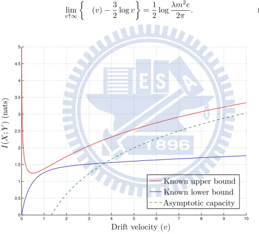
From (6.5) and (6.7), we can observe that the upper and the lower bound coincide, which proves the following result:

Theorem 6.1(Asymptotic Capacity of AIGN Channel with v Large). The capacity

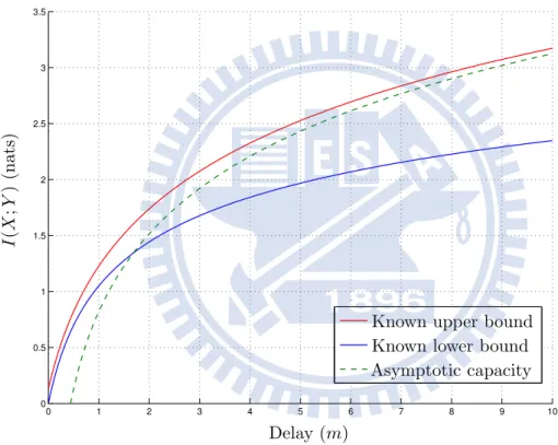
of the AIGN channel defined in Section 1.1 and 1.2 is asymptotically, when the drift velocity v of the fluid medium tends to infinity while all other parameters are kept constant, as follow: lim v↑∞ J (v)₋3 2log v K = 1 2log λm2_e 2π . (6.8) 0 1 2 3 4 5 6 7 8 9 10 0 0.5 1 1.5 2 2.5 3 3.5 4 4.5 5

Known upper bound Known lower bound

I (X ;Y ) (nat s) Drift velocity (v) Asymptotic capacity

Figure 6.14: Setting parameter: m = 2, d = 1 and σ2_{= 1.}

6.2

When m Large

First, we use the known upper bound introduced in Chapter 3 since it is also asymp-totically tight in m: (m)≤ 1 + log(m + µ) − hIG(µ,λ) (6.9) = 1 + log m + log)1 + µ m * − hIG(µ,λ), (6.10)

where h(N ) is independent of m. When m goes to infinity, the upper bound becomes: (m)≤ log m + 1 2log eλ 2πµ3 − 3 2e 2λ µ _Ei # −2λ µ $ + o(1) (6.11)

On the other hand, we also pick the lower bound in Section 4.3.

(m)_{≥ log}m λ + µ m− λ µ + kλ + 3 2log λ µ+ 1 2log e 2π− 3 2e 2λ µ Ei # −2λ µ $ − log / 1 + 1 me λ µ 1 λm 2 + k2_λm 1 /1 2λ m + k2λ2 0 + 1 2me λ µ+kλ 1 λm 1 + k2_λm 1 / 21 λ m+ k 2_λ2 00 (6.12) = log m +1 2log eλ 2πµ3 − 3 2e 2λ µ Ei # −2λ µ $ + o(1) (6.13)

where k =(_µ12 −_λm2 . Here, (6.13) is because the last term of (6.12) goes to 0 once

we let m goes to infinity. From (6.11) and (6.13), we can observe that the upper and the lower bound coincide, which proves the following result.

Theorem 6.2(Asymptotic Capacity of AIGN Channel with m Large). The capacity

of the AIGN channel defined in Section 1.1 and 1.2 is asymptotically, when the average-delay constraint m is loosened to infinity while all other parameters are kept constant, as follow: lim m↑∞{ (m) − log m} = 1 − hIG(µ,λ) (6.14) = 1 2log λe 2πµ3 − 3 2exp # 2λ µ $ Ei # −2λ_µ $ . (6.15)

Chapter 6 Asymptotic Capacity of AIGN Channel 0 1 2 3 4 5 6 7 8 9 10 0 0.5 1 1.5 2 2.5 3 3.5

Known upper bound Known lower bound

I (X ;Y ) (nat s) Delay (m) Asymptotic capacity

Discussion and Conclusion

In this thesis, a new type of channel, the additive inverse Gaussian noise channel, has been investigated. We introduced its interesting properties and related lemmas. Several methods of upper-bounding and lower-bounding its channel capacity are provided.

We have found out that the upper bounds (3.15) and (3.16) from literature [1] are very tight by providing analytical lower bound that is tight in the asymptotic regime. Therefore, we focused on the low drift velocity v and low average-delay m

regime. Note that (3.16) has a strange increasing behavior when v _{→ 0. Here we}

provided an upper bound (5.40) that is better than (3.16) in low v. Moreover, (3.15)

does not tend to 0 as m → 0, while we can show an improved upper bound (5.40)

that does tends to 0.

The lower bounds (3.15) and (3.14) in [1], are not tight enough in both high v and high m. With the help of [10], we were able to compute the exact output distribution of an exponential input. This lower bound (4.82) was much tighter than the known bound with respect to both v and m. It turned out that together with the known upper bound, this lower bound allowed us to derive the asymptotic capacity at high v (6.8) and m (6.15).

For future research, we propose the following problems related to the additive inverse Gaussian noise channel:

• Derivation of the exact slope of the asymptotic capacity when m → 0. • Derivation of the channel capacity behavior for v → 0.

• Inclusion of a peak-delay constraint to the system. • Extension to nonadditive channels.

Bibliography

[1] K. V. Srinivas, Raviraj S. Adve, and Andrew W. Eckford, “Molecular communi-cation in fluid media: The additive inverse Gaussian noise channel,” December 2010, arXiv:1012.0081v2 [cs.IT]. [Online]. Available: http://arxiv.org/abs/101 2.0081v2

[2] Claude E. Shannon, “A mathematical theory of communication,” Bell System Technical Journal, vol. 27, pp. 379–423 and 623–656, July and October 1948. [3] I. S. Gradshteyn and I. M. Ryzhik, Table of Integrals, Series, and Products,

6th ed., Alan Jeffrey, Ed. San Diego: Academic Press, 2000.

[4] Raj S. Chhikara and J. Leroy Folks, The Inverse Gaussian Distribution — Theory, Methodology, and Applications. New York: Marcel Dekker, Inc., 1989. [5] V. Seshadri, The Inverse Gaussian Distribution — A Case Study in Exponential

Families. Oxford: Clarendon Press, 1993.

[6] Toshihiko Kawamura and Kosei Iwase, “Characterizations of the distributions of power inverse Gaussian and others based on the entropy maximization princi-ple,” Journal of the Japan Statistical Society, vol. 33, no. 1, pp. 95–104, January 2003.

[7] Thomas M. Cover and Joy A. Thomas, Elements of Information Theory, 2nd ed. New York: John Wiley & Sons, 2006.

[8] Norman L. Johnson and N. Balakrishnan, Advances in the Theory and Practice of Statistics. New York: John Wiley & Sons, 1997.

[9] Stefan M. Moser, Duality-Based Bounds on Channel Capacity, ser. ETH Series in Information Theory and its Applications. Konstanz: Hartung-Gorre Verlag, January 2005, vol. 1, ISBN 3–89649–956–4, edited by Amos Lapidoth. [Online]. Available: http://moser.cm.nctu.edu.tw/publications.html

[10] Wolf Schwarz, “On the convolution of inverse Gaussian and exponential ran-dom variables,” Communications in Statistics — Theory and Methods, vol. 31, no. 12, pp. 2113–2121, 2002.

[11] Amos Lapidoth, Stefan M. Moser, and Mich`ele Wigger, Advanced Optical

Wire-less Communication Systems. Cambridge: Cambridge University Press, May