由結構推導蛋白質與蛋白質接觸面的動力學特性

(1)

國立交通大學

生物資訊及系統生物研究所

碩士論文

由結構推導蛋白質與蛋白質接觸面的動力學特性

Structure-derived dynamic properties of

protein-protein interfaces

研究生：林子琳

指導教授：黃鎮剛教授

(2)

i

由結構推導蛋白質與蛋白質接觸面的動力學特性

研究生: 林子琳指導教授: 黃鎮剛教授國立交通大學生物資訊及系統生物研究所

摘要

蛋白質的交互作用完成了許多生物功能。序列研究指出蛋白質與蛋白質作用區富含厭水性胺基酸；然而，目前為止蛋白質的結構資訊尚無法清楚地區分蛋白質與蛋白質的接觸面與其他蛋白質表面。我們在這個研究中分析了兩項與動力學相關的結構資訊: 蛋白質與蛋白質接觸面的中心與蛋白質的質心距離比一般蛋白質表面與蛋白質的質心距離小。蛋白質與蛋白質接觸面的中心的加權接觸數目比一般蛋白質表面的加權接觸數目大。這表示蛋白質與蛋白質接觸面的中心是靠近蛋白質的質量中心並且處於擁擠的堆疊狀態。

(3)

ii

Structure-derived dynamic properties of protein-protein interfaces

Student: Zih-Lin Lin Advisor: Dr. Jenn-Kang Hwang

National Chiao Tung University

Institute of Bioinformatics and Systems Biology

Abstract

Many biological functions result from the interactions between proteins. From

sequence information, studies have revealed that the interaction interfaces are

conserved in hydrophobic environments. However, structure information is still not

clear enough to differentiate interaction interfaces from protein surfaces. In this study,

we analyzed two structural properties related to protein dynamics: the core interface

residues are closer to the centroid of protein, and the weighted contact numbers of

core interface residues are larger than that of surface residues. The results suggest that

the core interface residues are nearness to the protein centroid and in a crowded

(4)

iii

誌謝

謝謝大家!!感恩幫助我完成論文，兩年以來給我支持與鼓勵的所有人!!首先要感謝的是提供我研究機會的黃鎮剛老師，給予我研究上的指教，指點我學術上的迷津，並且鼓勵我以樂觀的想法與不同的角度看待自己的實驗成果。感謝老師讓我了解作研究應有的態度與方法也教導我待人接物的道理。接著我要感謝實驗室研究同仁們：景盛，志豪，志鵬，建華，存操，啟文，彥龍，士中，儼毅，仙蕾，人維對我在程式與實驗設計方面的指導與幫助以及協助我的口試的進行。還有實驗室的研究同仁們：少偉，志杰，肇基，瓊文，松桓，曉芬，乃文，儷芬在我研究生活上的幫忙助益。還要感謝系上朋友們：智先，志偉，慶恩，宗翰，彥修，敬立，廖芹，佳達，昭昉，致宏，在我研究遇到瓶頸時給我的支持與鼓勵。另外，我要特別感謝:志鵬學長，存操學長，啟文學長，士中學長，仙蕾學姊協助我設計實驗也教導我程式邏輯與應用，並且幫助我撰寫論文，教了我實驗低潮時應抱持正面樂觀的態度。我也要感謝我的家人在我背後的支持，還有之義在我旁邊幫我搖旗加油，以及我的愛鼠賈修在新竹陪伴我。紙短情長，再次感謝所有幫助我與陪伴我的人們。

(5)

iv

Introduction

Classifying residues as surface exposed and buried, based on their solvent

accessibilities, is a simple but important step towards understanding the contributions

of the residues to the structural integrity1-2. Surface exposed residues are often crucial

for interactions with other proteins and play functional roles while the buried residues

contribute more towards stability of the tertiary structures3. Proteins perform their

function by interacting with other molecules, such as small ligands, lipids, nucleic

acids, and other proteins4. The recognition of protein-protein interaction sites can be

used to identify functionally important amino acid residues, facilitate experimental

efforts to catalog protein interactions, enhance computational docking studies and

drug designs, as well as enable functional annotation for the growing number of

structurally resolved proteins of unknown functions4.

Identification of the interface between interacting proteins is an important clue to

the function of a protein. In general, the problem of recognition of protein–protein

interaction sites can be cast as a classification problem, that is, each amino acid

residue is assigned to one of two classes: interacting (interfacial) or non-interacting

(non-interfacial) residues4. The experimental methods such as yeast-two-hybrid

screening, immune-precipitation assays and Föster resonance energy transfer (FRET)

(7)

2

but it is still difficult to use above experimental methods to identify which residues

are in the interaction region, called interface. By analyzing the surfaces of proteins,

the interfaces can be differentiated from the surfaces of component subunits in protein

complexes.

The characteristics of interface residues have been systematically studied. Lo

Conte and Chothia et al.8 have analyzed the amino acid compositions of

protein-protein complexes. They discovered the interface residues are more aliphatic

and aromatic than the rest part of protein surface. Neuvirth et al.9 noticed that polar

and hydrophobic residues are more plentiful in the interface than the rest part of

surface. Tyr, Met, Cys, and His are favored on binding interface9. Zhou and Shan et

al.10 observed that the interface residues are apparently more conserved than the

non-interfacial surface residues.

The protein dynamics tell us the information about how the protein moves. It is

well-known that protein dynamics is highly correlated to protein function. The

experimental measurement of the oscillations of an atom around its mean position in a

protein structure is called B-factor. The B-factor (also called crystallographic

temperature factor and Debye-Waller factor) in protein X-ray structures is an

experimental evidence to protein structure dynamics and is closely related to the

(8)

3

B-factor of proteins in free form and revealed that the B-factor of interface is slightly

lower than that of the surface in the unbound state9. This result is consistent with the

finding that an interfacial surface region is less flexible than the rest of the protein

surface in unbound state12.

The protein dynamics are usually calculated by mechanical models. Molecular

dynamics (MD) simulation is one of the most famous mechanical models used to

describe protein flexibility. Molecular dynamics computes the movements of proteins

based on bond stretching, bond angle bending, bond twisting, van der Waals and

electrostatic interaction13-15. The main drawback of MD simulation is its high

computational cost16-17. Several prediction methods for protein dynamics elaborated

based on protein structures overcame this limitation. For example, the centroid model

(CM)18 and weighted contact number model (WCN)19 developed by our group. The

CM computes protein dynamics directly from the protein geometrical shape. The CM

method is based on the observation that the deeper an atom is buried inside a protein

structure, the less it will fluctuate around its equilibrium position18. The CM only

computes the coordinates of Catoms and plainly defines the center of mass of a protein. The distance square between the C atoms to the center of mass of the protein is accordant to the thermal fluctuation. The atomic fluctuation is in fact

(9)

4

protein18. The weighted contact number model (WCN) calculates the number of

neighbor atoms which is weighted by inverse distance between two atoms of each pair.

The WCN computes protein dynamics from the protein packing. If an atom is more

crowded in a protein structure, the less it will fluctuate around its equilibrium

position19. We use the CM and WCN to analysis the differences between interfaces

and the rest part of the surfaces. We applied the two methods to protein-protein

complexes and found the correlation between protein dynamics and interface residues.

In the work presented here, the distance to the protein centroid and the weighted

contact number were analyzed for both interfaces and surfaces. These two structural

(10)

5

Materials and Methods

We use the ProMate database and ZW databases to analyze the components of

protein interface residues and surface residues. And we have further defined the

interface residues as core interface residues and peripheral interface residues. Core

interface develops the center region of interface and peripheral interface contrasts the

rim area of interface. The core interface and peripheral interface together form the

interface. We analysis the components and tendencies of core interface and peripheral

interface.

ProMate database

ProMate database9 contains 57 protein-protein interaction structures. The

database consists of both the unbound and bound states for transient protein-protein

hetero-dimers derived from the PDB20. The unbound and bound states of proteins

were determined by X-ray crystallography or NMR. The ProMate database has 42

X-ray structures protein structures in unbound form.

The ProMate database was extracted from a database of 92 bound monomers

longer than 85 AA. The combinatorial extension method (CE)21 was prosecuted to

find each possible pair of monomers and one of them would be executed from

(11)

6

The unbound structures were then derived from the bound structures. 57

monomers in bound form were found to have a highly homologous unbound form in

the PDB20 by using BLAST22, with more than 70% sequence identity.

ZW database

The ZW dataset contains 101 transient protein-protein complexes. The 101

transient protein-protein complexes were retrieved from the Zhiping Weng’s transient

databases23. The Zhiping Weng group had collected 212 non-redundant transient

hetero-dimeric X-ray structures of protein-protein interactions24.

To obtain data for hetero-dimers, the Zhiping Weng group only kept the records

of X-ray structures better than 3.25 Å and all the chains in the database are longer

than 25 amino acids. They eliminated all homomeric records using the

BLASTCLUST algorithm25. A homomeric record was defined which all chains have

85% sequence identity to each other and at least 50% of the sequence was aligned. To

receive a non-redundant database of protein complexes, they used pairwise BLAST22

to check each pair of all chains in the database and deleted one complex of the pair

with 25% sequence identity.

And we have further used global sequence alignment to check each pair of each

(12)

7

identity. We remained 101 transient protein-protein complexes in the ZW database.

Surface and interface definition

We took the bound state complexes apart and treated the subunits as the unbound

state of complexes. After clarifying the corresponding residues between unbound state

and bound state for protein-protein complexes, we explored the surface residues and

interface residues.

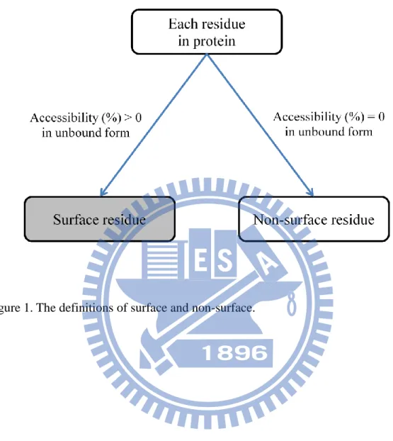
The accessibility(%) plays an important role in definition of surface and interface.

Accessibility(%) is presented as

𝐴𝑐𝑐𝑒𝑠𝑠𝑖𝑏𝑖𝑙𝑖𝑡𝑦𝑖(%) =

𝑆𝐴𝑖

𝑆𝑡𝑎𝑛𝑑𝑎𝑟𝑑 𝑆𝐴𝑖100% (1)

Accessibility(%) of the i-th residue, 𝐴𝑐𝑐𝑒𝑠𝑠𝑖𝑏𝑖𝑙𝑖𝑡𝑦𝑖(%), is defined as the ratio of the

solvent exposed surface area of the i-th residue. SAi is the solvent exposed surface

area of the i-th residue and Standard SAi is the standard value of the solvent exposed

surface area for this kind of amino acid26. We use the DSSP program27 to calculate

exposed surface areas in unbound state and bound state of protein-protein complexes.

We defined the surface residue based on the accessibility(%) in unbound state and the

interface residue based on the delta accessibility(%) upon complex formation28. A

residue was categorized as a surface residue if its accessibility(%) in free form is

(13)

8

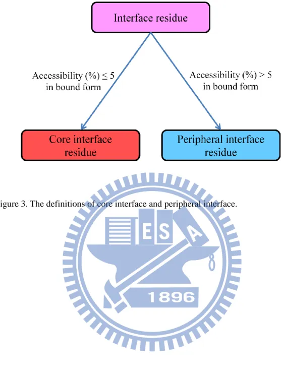
upon complex formation. And we further separated interfaces as core interfaces and

peripheral interfaces based on the accessibilities(%) in bound state. If an interface

residue has the accessibility(%) in the complex smaller than or equal to 5, it is a core

interface residue, else it is a peripheral interface residue. An interface residue is taken

as either a core interface residue or a peripheral interface residue. The definition of

surface, interface, core interface and peripheral interface are showed in Figure

1~Figure 3, and one example is pictured in Figure 4.

Amino acid components

We have calculated the amino acid propensities using the following equations: 𝑃𝑟𝑜𝑝𝑒𝑛𝑠𝑖𝑡𝑦_{𝑇𝑎𝑟𝑔𝑒𝑡} = 𝑂𝑐𝑐𝑢𝑟𝑒𝑛𝑐𝑒 𝑇𝑎𝑟𝑔𝑒𝑡

𝑂𝑐𝑐𝑢𝑟𝑒𝑛𝑐𝑒𝑆𝑢𝑟𝑓𝑎𝑐𝑒 (2)

Where 𝑃𝑟𝑜𝑝𝑒𝑛𝑠𝑖𝑡𝑦_{𝑇𝑎𝑟𝑔𝑒𝑡} is the amino acid type propensity of the target residues.

𝑂𝑐𝑐𝑢𝑟𝑒𝑛𝑐𝑒_{𝑇𝑎𝑟𝑔𝑒𝑡}, 𝑂𝑐𝑐𝑢𝑟𝑒𝑛𝑐𝑒_{𝑆𝑢𝑟𝑓𝑎𝑐𝑒} are the amino acid type occurrences of the

target residues and the surface residues.

Secondary structure definition

The secondary structure is defined by DSSP27 program. DSSP recognizes eight

types of secondary structure, depending on the pattern of hydrogen bonds and 3D

(14)

9 H: -helix

B: residue in isolated -bridge

E: extended strand, participates in  ladder G: 3/10 helix

I: -helix

T: hydrogen bonded turn

S: bend

U: undefined

These eight types are usually grouped into three larger classes: helix (G,H, and I),

strand (E and B), and loop (all others).

Centroid Model (CM)

Let X0 be the center of mass of the protein, which is express as

𝑋0 = 𝑚𝑘 𝑘𝑋𝑘/ 𝑚𝑘 𝑘 (3)

Where mk and Xk are the mass and the crystallographic position of C atom k, respectively. The distance of the C atom i from the center of mass of the protein is expressed as

𝑟_𝑖2 = X_i− X₀ X_i− X₀ (4)

(15)

10

of size N has the square distance of each C atom given by (𝑟₁2, 𝑟₂2, … , 𝑟_𝑛2). The r2 profile is closely related to the thermal B-factor, which is given as

𝐵𝑖 = ( 8𝜋2

3 )(𝛿𝑋𝑖𝛿𝑋𝑖) (5)

The centroid model suggest the following interesting relation,

𝛿𝑋_𝑖𝛿𝑋_𝑖 ~ 𝑋𝑖 − 𝑋0 𝑋𝑖− 𝑋0 (6)

And equation (5) and (6) suggests that the fluctuation of a residue is usually

proportional to the distance between center of mass and its position.

Weighted Contact-Number model (WCN)

When the neighboring contact number of an atom is larger, the fluctuation of the

atom will be smaller. We can define WCN model as

𝑉𝑖 = 𝑁𝑗 ≠𝑖( 1/𝑟𝑖𝑗2) (7)

The equation (7) defines 𝑉_𝑖, the number of C atoms which surround the 𝑖𝑡𝑕 residue.

The influence of atom j to the atom i is attenuated by the factor 1/𝑟𝑖𝑗2. rij is the

distance between C atoms of residues i and j.

Z-score

On the mission to compare the results, we would normalize the 𝑟𝑖2 of CM and

(16)

11

𝑧_𝑥_𝑖 = (𝑥_𝑖 − 𝑥 )/𝜎_𝑥 (8)

𝑥 is the mean of x and is the standard deviation of x, where the 𝑥_𝑖 represents

the 𝑟_𝑖2_{of CM and}_𝑣

𝑖 of WCN.

Two-sample t-test

To compare the differences between interfaces and the rest part of the surfaces,

we use the two-sample t-test. 𝑡 = 𝑥 −𝑦

𝑠𝑥 2_𝑚+𝑠𝑦 2

𝑛

(9)

Where 𝑥 and 𝑦 are the sample means, sx and sy are the sample standard deviations,

and m and n are the sample sizes of the two groups. When a t is determined, a p-value could be decided from the Student’s t-distribution table. If the p-value is lower than 0.05, the two sample have differences.

(17)

12

Results and Discussions

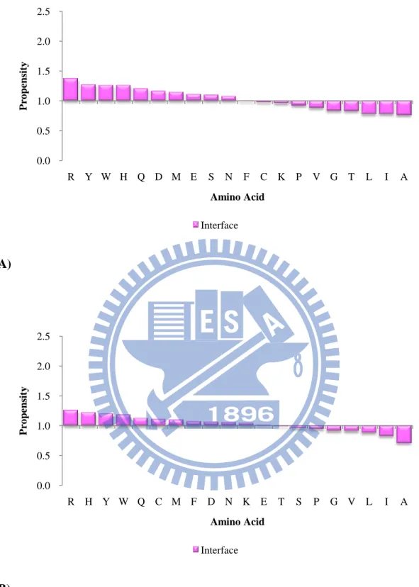
Amino acid components

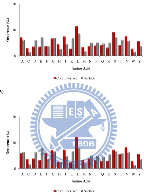
The amino acid distributions of core interfaces, peripheral interfaces and

interfaces could give a general indication of relative importance of different amino

acids. Percentage frequencies and propensities of amino acids were calculated for

each amino acid type and the results were illustrated in Figure 5~10.

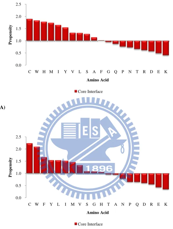
Cys, Trp, His, Met, Ile are the most dominant amino acid types in the core

interface in the ProMate database and Cys, Trp, Phe, Tyr, and Leu are the most

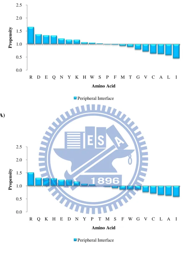
abundant amino acids in the core interface in the ZW dataset. Arg, Asp, Glu, Gln, and

Asn are the most dominant amino acids in the peripheral interfaces in the ProMate

database. Arg, Glu, Lys, His and Glu are the most dominant amino acids in the

peripheral interfaces in the ZW database. We could observed that the core interface

prefers polar, uncharged and aromatic amino acids whereas the peripheral interface

likes charged residues.

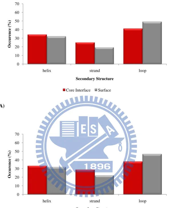
Secondary structure constituents

The occurrences of secondary structures are represented in Figure 11~13. The

rigid secondary structures, helices and strands, are preferred in the core interfaces

(18)

13

in the core interfaces contract to surfaces. The flexible secondary structures, loops, are

preferred in the peripheral interfaces compared with surfaces and the rigid secondary

structures, helices and strands, are unfavorable in the peripheral interfaces contract to

surfaces.

Accessibilities and delta accessibilities

The accessibility distributions in unbound state are pictured in Figure 14~16. The

accessibilities of core interfaces are lower than that of surfaces and the accessibilities

of peripheral interfaces are higher than that of surfaces. The analysis of accessibilities

revealed that the peripheral interfaces are significantly more accessible than the rest of

surfaces.

The delta accessibilities in complexation are pictured in Figure 17~18. There is

no difference of delta accessibility distributions between core interfaces, peripheral

interfaces, and interfaces.

Evolutionary conservation

It is interesting to research the conservation degree of proteins if the

protein-protein interactions play important part in function. We measured the

(19)

14

corresponds to its evolutionary rate. The residues evolve slowly are directed to be

conserved residues. The lower the conservation score obtained from ConSurf, the

higher the conservation degree the residue has.

We could see that the conservation scores are much lower in the core interfaces

in Figure 19. The p-values between core interfaces and surfaces in the ProMate

database and the ZW database are both 0.00. Figure 20 represents that there is no

difference between the conservation scores of peripheral interface and surface. The

p-values between peripheral interfaces and surfaces in the ProMate database and the

ZW database are 2.39× 10-2, and 5.30 × 10-3 sequentially. Figure 21 shows the

tendencies of conservation scores of interface and surfaces. We could see that the

conservation scores are lower in the interfaces than that in the surfaces. The p-values

of conservation scores of the ProMate database, the ZW database are 1.33 × 10-5,

1.66× 10-11 sequentially. The analysis of conservation scores revealed that the core

interfaces play important roles in protein-protein interactions and the core interfaces

are more conserved than the rest part of surfaces.

B-factors

The X-ray crystallization structures from Protein Data Bank offer the B-factor

(20)

15

experiments and related to protein structure dynamics. The higher the B-factor the

residue has, the more flexible the residue is.

We analyzed the B-factor distributions in unbound form of the ProMate database.

We used the EMBOSS Pairwise Alignment Algorithm30 to search for regions of local

similarity and homologous residues between the two sequences of unbound state and

bound state for protein-protein complexes. We found that the B-factors in unbound

form of core interfaces are significantly lower than that of surfaces (Figure 22) and

the t-test comparing core interfaces and surfaces gave a p-value of 1.07 × 10-10. The

B-factors in unbound form of peripheral interfaces are slightly higher than that of

surfaces (Figure 23) and the p-value is 1.31 × 10-10. The B-factors of interfaces have

no difference with that of surfaces (Figure 24) and the p-value is 3.97 × 10-2. We

could notice greatly dissimilarity between core interface and surfaces. We could

observed from the B-factor presences that the core interfaces are more rigid than the

surfaces and the peripheral interfaces are slightly elastic than the surfaces in unbound

state.

Figure 31 depicts the protein structure of pdbid 1tmq. We could exam the

B-factors of core interface and peripheral interfaces of the chain A of 1tmq in the

upper figure. The B-factors of 1tmqA were obtained from the homologous protein of

(21)

16

expresses low B-factor values respectively. We could contract the upper and lower

figures and perceive that the B-factors of core interfaces are much lower than that of

the rest of the surfaces.

Centroid Model (CM)

The centroid model (CM) only computes the distance square between each C atom to the center of mass of the protein. The CM method is based on the observation

that the deeper an atom is buried inside a protein structure, the less it will fluctuate

around its equilibrium position.

We measured the CM distributions of protein-protein interactions in unbound

state. The CM of the core interfaces is significantly lower than the CM of the surfaces

in unbound form (Figure 25) and the p-values of ProMate database, ZW database both

are 0.00. The CM of the peripheral interfaces is lightly higher than the CM of the

surfaces in unbound form (Figure 26) and the p-values of ProMate database, ZW

database are 2.77 × 10-6, and 0.00. The CM distributions have no significant

difference between the interfaces and the surfaces (Figure 27). The two sample t-test

gave p-values between the interfaces and surfaces of the two databases with 3.16 ×

10-1, 2.70 × 10-4. The core interfaces are close to the center of mass of protein

(22)

17

center of mass of protein structures are slightly longer than that between surfaces and

the center of mass of protein structures.

Visualization of the example of CM model was described in Figure 32. The

average distance between surfaces and the center of mass of 1tmqA is 22.62 Å . The

distance between the core interface residue, W56, and the center of mass is 16.79 Å .

The distance between the peripheral interface residue, E229, and the center of mass is

24.62 Å . The distances of the core interfaces are shorter than that of the surfaces.

Weighted Contact Number model (WCN)

The weighted contact number model (WCN) estimates protein dynamics by

calculating the protein packing denseness. The WCN model computes the number of

neighboring atoms which is weighted by inverse distance between two atoms of each

pair. The WCN is based on that the more crowded an atom is around its environment

in a protein structure, the less it will swing around its equilibrium position.

Examining Figure 28 reveals that core interfaces have much higher WCN than

the whole surfaces. The two sample t-test contrast the core interfaces and the whole

surfaces and gave both p-values of 0.00 in the ProMate database and the ZW database.

Figure 29 shows that peripheral interfaces have much lower WCN than the whole

(23)

18

surfaces and gave both p-values of 0.00 in the ProMate database and the ZW database.

Observing Figure 30 reveals that the interfaces have lower WCN than the whole

surfaces. The two sample t-test contrast the interfaces and the whole surfaces and

gave p-values of 7.54 × 10-13

, 0.00 individually in the ProMate database, the ZW

database. The core interfaces have high packing densities and the peripheral interfaces

have low packing densities in unbound state.

We could also observe from Figure 33 that the core interfaces are sunken on the

surface and the peripheral interfaces are protruding on the surface. The example of

Figure 33 agrees with the results of WCN model. It shows that core interface is in a

crowded environment and the peripheral interface is not.

Summary

The results of B-factors, WCN, CM suggest that the core interfaces are rigid and

the peripheral interfaces are plastic on the surface. The analysis of protein secondary

structures also supports the dynamic observations. The evolutionary conservation

measurements exposed that the core interfaces are more conserved in the surface

whereas the peripheral interfaces are not. It means the core interfaces play important

role in protein-protein interactions.

(24)

19

protein-protein interaction are rigid. And we could further use these structure

(25)

20

References

1. Pollastri G, Baldi P, Fariselli P, Casadio R. Prediction of coordination number and relative solvent accessibility in proteins. Proteins 2002;47(2):142-153. 2. Rost B, Sander C. Conservation and prediction of solvent accessibility in

protein families. Proteins 1994;20(3):216-226.

3. Chan HS, Dill KA. Origins of structure in globular proteins. Proc Natl Acad Sci U S A 1990;87(16):6388-6392.

4. Porollo A, Meller J. Prediction-based fingerprints of protein-protein interactions. Proteins 2007;66(3):630-645.

5. Young KH. Yeast two-hybrid: so many interactions, (in) so little time. Biol Reprod 1998;58(2):302-311.

6. Crowell RE, Du Clos TW, Montoya G, Heaphy E, Mold C. C-reactive protein receptors on the human monocytic cell line U-937. Evidence for additional binding to Fc gamma RI. J Immunol 1991;147(10):3445-3451.

7. Jares-Erijman EA, Jovin TM. FRET imaging. Nat Biotechnol 2003;21(11):1387-1395.

8. Lo Conte L, Chothia C, Janin J. The atomic structure of protein-protein recognition sites. J Mol Biol 1999;285(5):2177-2198.

9. Neuvirth H, Raz R, Schreiber G. ProMate: a structure based prediction program to identify the location of protein-protein binding sites. J Mol Biol 2004;338(1):181-199.

10. Zhou HX, Shan Y. Prediction of protein interaction sites from sequence profile and residue neighbor list. Proteins 2001;44(3):336-343.

11. Halle B. Flexibility and packing in proteins. Proc Natl Acad Sci U S A 2002;99(3):1274-1279.

12. Jones S, Thornton JM. Protein-protein interactions: a review of protein dimer structures. Prog Biophys Mol Biol 1995;63(1):31-65.

13. Levitt M, Warshel A. Computer simulation of protein folding. Nature 1975;253(5494):694-698.

14. Warshel A. Bicycle-pedal model for the first step in the vision process. Nature 1976;260(5553):679-683.

15. McCammon JA, Gelin BR, Karplus M. Dynamics of folded proteins. Nature 1977;267(5612):585-590.

16. Pandey BP, Zhang C, Yuan X, Zi J, Zhou Y. Protein flexibility prediction by an all-atom mean-field statistical theory. Protein Sci 2005;14(7):1772-1777. 17. Rueda M, Ferrer-Costa C, Meyer T, Perez A, Camps J, Hospital A, Gelpi JL,

(26)

21 2007;104(3):796-801.

18. Shih CH, Huang SW, Yen SC, Lai YL, Yu SH, Hwang JK. A simple way to compute protein dynamics without a mechanical model. Proteins 2007;68(1):34-38. 19. Lin CP, Huang SW, Lai YL, Yen SC, Shih CH, Lu CH, Huang CC, Hwang JK.

Deriving protein dynamical properties from weighted protein contact number. Proteins 2008;72(3):929-935.

20. Berman HM, Westbrook J, Feng Z, Gilliland G, Bhat TN, Weissig H, Shindyalov IN, Bourne PE. The Protein Data Bank. Nucleic Acids Res 2000;28(1):235-242. 21. Shindyalov IN, Bourne PE. Protein structure alignment by incremental

combinatorial extension (CE) of the optimal path. Protein Eng 1998;11(9):739-747.

22. Altschul SF, Madden TL, Schaffer AA, Zhang J, Zhang Z, Miller W, Lipman DJ. Gapped BLAST and PSI-BLAST: a new generation of protein database search programs. Nucleic Acids Res 1997;25(17):3389-3402.

23. Mintseris J, Weng Z. Structure, function, and evolution of transient and obligate protein-protein interactions. Proc Natl Acad Sci U S A 2005;102(31):10930-10935.

24. Mintseris J, Weng Z. Atomic contact vectors in protein-protein recognition. Proteins 2003;53(3):629-639.

25. Johnson M, Zaretskaya I, Raytselis Y, Merezhuk Y, McGinnis S, Madden TL. NCBI BLAST: a better web interface. Nucleic Acids Res 2008;36(Web Server issue):W5-9.

26. Rose GD, Geselowitz AR, Lesser GJ, Lee RH, Zehfus MH. Hydrophobicity of amino acid residues in globular proteins. Science 1985;229(4716):834-838. 27. Kabsch W, Sander C. Dictionary of protein secondary structure: pattern

recognition of hydrogen-bonded and geometrical features. Biopolymers 1983;22(12):2577-2637.

28. Jones S, Thornton JM. Analysis of protein-protein interaction sites using surface patches. J Mol Biol 1997;272(1):121-132.

29. Landau M, Mayrose I, Rosenberg Y, Glaser F, Martz E, Pupko T, Ben-Tal N. ConSurf 2005: the projection of evolutionary conservation scores of residues on protein structures. Nucleic Acids Res 2005;33(Web Server issue):W299-302.

30. Smith TF, Waterman MS. Identification of common molecular subsequences. J Mol Biol 1981;147(1):195-197.

(27)

22

Figures

(28)

23

(29)

24

(30)

25

(A)

(B)

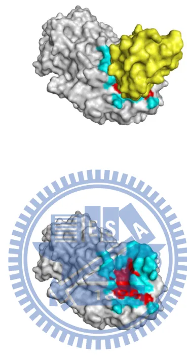
Figure 4. Visualization of the core interface and the peripheral interface (PDB entry 1tmq) (A) Chain A and chain B. (B) Chain A only. Visual graphics tool

Pymol was used to visualize the core interface and peripheral interface of 1tmqA. The

chain A was shown in gray and chain B was shown in yellow. The core interface and

(31)

26

(A)

(B)

Figure 5. Comparison of the amino acid distributions between core interfaces and

surfaces in unbound state of (A) the ProMate database (B) the ZW database. 0 10 20 A C D E F G H I K L M N P Q R S T V W Y O cc urence ( %) Amino Acid Core Interface Surface

0 10 20 A C D E F G H I K L M N P Q R S T V W Y O cc urence ( %) Amino Acid Core Interface Surface

(32)

27

(A)

(B)

Figure 6. The amino acid propensities of core interfaces in unbound state of (A) the

ProMate database (B) the ZW database. 0.0 0.5 1.0 1.5 2.0 2.5 C W H M I Y V L S A F G Q P N T R D E K P ro pens it y Amino Acid Core Interface 0.0 0.5 1.0 1.5 2.0 2.5 C W F Y L I M V S G H T A N P Q D R E K P ro pens it y Amino Acid Core Interface

(33)

28

(A)

(B)

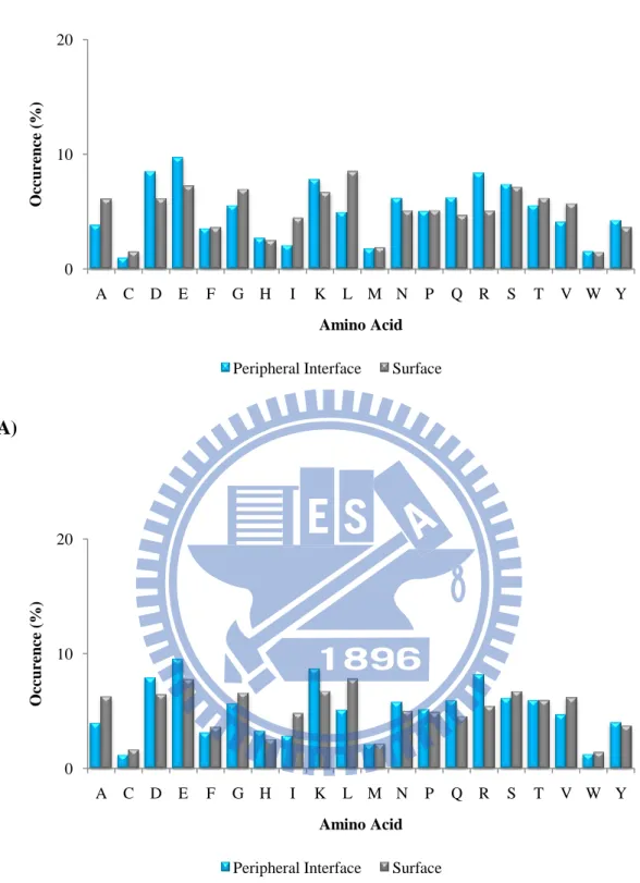
Figure 7. Comparison of the amino acid distributions between peripheral interfaces

and surfaces in unbound state of (A) the ProMate database (B) the ZW database. 0 10 20 A C D E F G H I K L M N P Q R S T V W Y O cc urence ( %) Amino Acid Peripheral Interface Surface

0 10 20 A C D E F G H I K L M N P Q R S T V W Y O cc urence ( %) Amino Acid Peripheral Interface Surface

(34)

29

(A)

(B)

Figure 8. The amino acid propensities of peripheral interfaces in unbound state of (A)

the ProMate database (B) the ZW database. 0.0 0.5 1.0 1.5 2.0 2.5 R D E Q N Y K H W S P F M T G V C A L I P ro pens it y Amino Acid Peripheral Interface 0.0 0.5 1.0 1.5 2.0 2.5 R Q K H E D N Y P T M S F W G V C L A I P ro pens it y Amino Acid Peripheral Interface

(35)

30

(A)

(B)

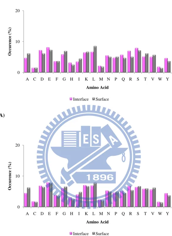
Figure 9. Comparison of the amino acid distributions between interfaces and surfaces

in unbound state of (A) the ProMate database (B) the ZW database. 0 10 20 A C D E F G H I K L M N P Q R S T V W Y O cc urence ( %) Amino Acid Interface Surface 0 10 20 A C D E F G H I K L M N P Q R S T V W Y O cc urence ( %) Amino Acid Interface Surface

(36)

31

(A)

(B)

Figure 10. The amino acid propensities of interface in unbound state of (A) the

ProMate database (B) the ZW database. 0.0 0.5 1.0 1.5 2.0 2.5 R Y W H Q D M E S N F C K P V G T L I A P ro pens it y Amino Acid Interface 0.0 0.5 1.0 1.5 2.0 2.5 R H Y W Q C M F D N K E T S P G V L I A P ro pens it y Amino Acid Interface

(37)

32

(A)

(B)

Figure 11. Comparison of the secondary structure distributions between core

interfaces and surfaces in unbound state of (A) the ProMate database (B) the ZW

database. 0 10 20 30 40 50 60 70

helix strand loop

O cc urence ( %) Secondary Structure Core Interface Surface

0 10 20 30 40 50 60 70

helix strand loop

O cc urence ( %) Secondary Structure

(38)

33

(A)

(B)

Figure 12. Comparison of the secondary structure distributions between peripheral

database. 0 10 20 30 40 50 60 70

helix strand loop

O cc urence ( %) Secondary Structure Peripheral Interface Surface

0 10 20 30 40 50 60 70

helix strand loop

O cc urence ( %) Secondary Structure Peripheral Interface Surface

(39)

34

(A)

(B)

Figure 13. Comparison of the secondary structure distributions between interfaces and

surfaces in unbound state of (A) the ProMate database (B) the ZW database. 0 10 20 30 40 50 60 70

helix strand loop

O cc urence ( %) Secondary Structure Interface Surface 0 10 20 30 40 50 60 70

helix strand loop

O cc urence ( %) Secondary Structure Interface Surface

(40)

35

(A)

(B)

Figure 14. Comparison of the distributions of solvent accessibility between core

database. 0 5 10 15 20 O cc urence ( %) Accessibility (%) Core Interface Surface

0 5 10 15 20 O cc urence ( %) Accessibility (%) Core Interface Surface

(41)

36

(A)

(B)

Figure 15. Comparison of the distributions of solvent accessibility between peripheral

database. 0 5 10 15 20 O cc urence ( %) Accessibility (%) Peripheral Interface Surface

0 5 10 15 20 O cc urence ( %) Accessibility (%) Peripheral Interface Surface

(42)

37

(A)

(B)

Figure 16. Comparison of the distributions of solvent accessibility between interfaces

and surfaces in unbound state of (A) the ProMate database (B) the ZW database. 0 5 10 15 20 O cc urence ( %) Accessibility (%) Interface Surface 0 5 10 15 20 O cc urence ( %) Accessibility (%) Interface Surface

(43)

38

(A)

(B)

Figure 17. Comparison of the distributions of accessibility change between core

interfaces and interfaces in complexation of (A) the ProMate database (B) the ZW

database. 0 5 10 15 20 25 O cc urence ( %) DAccessibility (%) Core Interface Interface

0 5 10 15 20 25 O cc urence ( %) DAccessibility (%) Core Interface Interface

(44)

39

(A)

(B)

Figure 18. Comparison of the distributions of accessibility change between peripheral

interfaces and interfaces in complexation of (A) the ProMate database (B) the ZW

database. 0 5 10 15 20 25 O cc urence ( %) DAccessibility (%) Peripheral Interface Interface

0 5 10 15 20 25 O cc urence ( %) DAccessibility (%) Peripheral Interface Interface

(45)

40

(A)

(B)

Figure 19. Comparison of the distributions of amino acid conservation scores between

core interfaces and surfaces in unbound state of (A) the ProMate database (B) the ZW

database. 0 10 20 30 40 -3 -2 -1 0 1 2 3 4 O cc urence ( %)

Conservation Score (normalized) Core Interface Surface

0 10 20 30 40 -3 -2 -1 0 1 2 3 4 O cc urence ( %)

Conservation Score (normalized) Core Interface Surface

(46)

41

(A)

(B)

peripheral interfaces and surfaces in unbound state of (A) the ProMate database (B)

the ZW database. 0 10 20 30 40 -3 -2 -1 0 1 2 3 4 O cc urence ( %)

Conservation Score (normalized) Peripheral Interface Surface

0 10 20 30 40 -3 -2 -1 0 1 2 3 4 O cc urence ( %)

Conservation Score (normalized) Peripheral Interface Surface

(47)

42

(A)

(B)

database. 0 10 20 30 40 -3 -2 -1 0 1 2 3 4 O cc urence ( %)

Conservation Score (normalized) Interface Surface 0 10 20 30 40 -3 -2 -1 0 1 2 3 4 O cc urence ( %)

Conservation Score (normalized) Interface Surface

(48)

43

Figure 22. Comparison of the B-factor distributions between core interfaces and

surfaces in unbound state of the ProMate database. 0 10 20 30 -2 -1 0 1 2 3 4 5 6 O cc urence ( %) B-factor (normalized) Core Interface Surface

(49)

44

Figure 23. Comparison of the B-factor distributions between peripheral interfaces and

surfaces in unbound state of the ProMate database. 0 10 20 30 -2 -1 0 1 2 3 4 5 6 O cc urence ( %) B-factor (normalized) Peripheral Interface Surface

(50)

45

Figure 24. Comparison of the B-factor distributions between interfaces and surfaces in

unbound state of the ProMate database. 0 10 20 30 -2 -1 0 1 2 3 4 5 6 O cc urence ( %) B-factor (normalized) Interface Surface

(51)

46

(A)

(B)

Figure 25. Comparison of the CM distributions between core interfaces and surfaces

in unbound state of (A) the ProMate database (B) the ZW database. 0 10 20 30 -2 -1 0 1 2 3 4 5 6 O cc urence ( %) CM (normalized) Core Interface Surface

0 10 20 30 -2 -1 0 1 2 3 4 5 6 O cc urence ( %) CM (normalized) Core Interface Surface

(52)

47

(A)

(B)

Figure 26. Comparison of the CM distributions between peripheral interfaces and

surfaces in unbound state of (A) the ProMate database (B) the ZW database. 0 10 20 30 -2 -1 0 1 2 3 4 5 6 O cc urence ( %) CM (normalized) Peripheral Interface Surface

0 10 20 30 -2 -1 0 1 2 3 4 5 6 O cc urence ( %) CM (normalized) Peripheral Interface Surface

(53)

48

(A)

(B)

Figure 27. Comparison of the CM distributions between interfaces and surfaces in

unbound state of (A) the ProMate database (B) the ZW database. 0 10 20 30 -2 -1 0 1 2 3 4 5 6 O cc urence ( %) CM (normalized) Interface Surface 0 10 20 30 -2 -1 0 1 2 3 4 5 6 O cc urence ( %) CM (normalized) Interface Surface

(54)

49

(A)

(B)

Figure 28. Comparison of the WCN distributions between core interfaces and surfaces

in unbound state of (A) the ProMate database (B) the ZW database. 0 10 20 30 -4 -3 -2 -1 0 1 2 3 O cc urence ( %) WCN (normalized) Core Interface Surface

0 10 20 30 -4 -3 -2 -1 0 1 2 3 O cc urence ( %) WCN (normalized) Core Interface Surface

(55)

50

(A)

(B)

Figure 29. Comparison of the WCN distributions between peripheral interfaces and

surfaces in unbound state of (A) the ProMate database (B) the ZW database. 0 10 20 30 -4 -3 -2 -1 0 1 2 3 O cc urence ( %) WCN (normalized) Peripheral Interface Surface

0 10 20 30 -4 -3 -2 -1 0 1 2 3 O cc urence ( %) WCN (normalized) Peripheral Interface Surface

(56)

51

(A)

(B)

Figure 30. Comparison of the WCN distributions between interfaces and surfaces in

unbound state of (A) the ProMate database (B) the ZW database. 0 10 20 30 -4 -3 -2 -1 0 1 2 3 O cc urence ( %) WCN (normalized) Interface Surface 0 10 20 30 -4 -3 -2 -1 0 1 2 3 O cc urence ( %) WCN (normalized) Interface Surface

(57)

52

(A)

(B)

Figure 31. Visualization of the B-factor of the core interface and the peripheral interface (PDB entry 1tmq) (A) The chain A of 1tmq was colored by B-factors. (B)

The chain A of 1tmq was colored in gray. The core interface and the peripheral

(58)

53

Figure 32. Visualization of the example of CM model (PDB entry: 1tmqA) The

core interface and peripheral interface were shown as sticks and colored in red and

cyan independently. The center of mass of chain A of 1tmq was pictured as sphere and

colored in green. The distance of the core interface residue, W56, and the center of

mass was 16.79 Å . The distance of the peripheral interface residue, E229, and the

(59)

54

(60)

55

Appendix

Homologous monomer Equivalent bound Homologous monomer Equivalent bound Homologous monomer Equivalent bound

1a19A 1brsD 1eza_ 3ezaA 1pne_ 1hluP

1a2pA 1brsA 1eztA 1agrE 1poh_ 1ggrB

1a5e_ 1bi7B 1f00I 1f02I 1ppp_ 1stfE

1acl_ 1fssA 1f5wA 1kacB 1qqrA 1bmlC

1ag6_ 2pcfA 1fkl_ 1b6cA 1rgp_ 1am4A

1aje_ 1am4D 1flzA 1euiA 1selA 1cseE

1ajw_ 1cc0E 1fvhA 1dn1A 1vin_ 1finB

1aueA 1fapB 1g4kA 1ueaA 1wer_ 1wq1G

1avu_ 1avwB 1gc7A 1ef1A 1xpb_ 1jtgA

1aye_ 1dtdA 1gnc_ 1cd9A 2bnh_ 1a4yA

1b1eA 1a4yB 1hh8A 1e96B 2cpl_ 1ak4A

1bip_ 1tmqB 1hplA 1ethA 2f3gA 1ggrA

1ctm_ 2pcfB 1hu8A 1ycsA 2nef_ 1avzB

1cto_ 1cd9B 1iob_ 1itbA 2rgf_ 1lfdA

1cye_ 1eayA 1j6zA 1c0fA 3ssi_ 2sicI

1d0nA 1c0fS 1jae_ 1tmqA 6ccp_ 2pcbA

1d2bA 1ueaB 1lba_ 1aroL 1jtgB

1ekxA 1d09A 1nobA 1kacA

1ex3A 1cgiE 1nos_ 1nocA

1ez3A 1dn1B 1pco_ 1ethB

(61)

56

2prg B:C 1ebd AB:C 1g0y I:R

1h59 A:B 1e6e A:B 1ijk A:BC

1c4z A:D 1gaq A:B 1n2c AB:EF

1evt A:C 1f80 A:E 1mah A:F

1dn1 A:B 1stf E:I 1gcq B:C

1xdt R:T 1f02 I:T 1www VW:X

1t7p A:B 2btc E:I 1i2m A:B

1go4 A:G 1gh6 A:B 1kgy A:E

1i85 B:D 1rlb ABCD:E 1c1y A:B

1jma A:B 1aro L:P 1gl4 A:B

1kac A:B 1ak4 A:D 1d2z A:B

1gc1 C:G 1i3o ABCD:E 3ygs C:P

1f51 AB:E 1atn A:D 1cs4 AB:C

1kmi Y:Z 1dkg AB:D 1efu A:B

7cei A:B 1b6c A:B 3sgb E:I

1bvn P:T 1qo0 A:DE 1fqv A:B

1qkz A:HL 1ugh E:I 1k3z AB:D

1dpj A:B 1df9 B:C 1m4u A:L

1f83 A:BC 1jiw I:P 1m2o AC:B

1fak HL:T 1f93 AB:EF 1mbu A:C

1jw9 B:D 1noc A:B 1fc2 C:D

1jtd A:B 1hwg A:BC 1ml0 A:D

1d5x A:C 1fg9 AB:C 1gvn AC:B

1i4e A:B 1ebp A:CD 1o6s A:B

1ib1 AB:E 1du3 A:DEF 1h2k A:S

2pcc A:B 1euv A:B 1m1e A:B

1f3v A:B 1de4 CF:A 1o94 AB:CD

1lpb A:B 1ghq A:B 1nf5 A:B

1ay7 A:B 1flt VW:X 1gzs A:B

1kkl ABC:H 1gxd A:C 1nbf A:D

1dev A:B 1ycs A:B 1mr1 A:D

1l0o AB:C 1gla F:G

1dfj E:I 2sic E:I

1g4y B:R 1jsu AB:C

1jch A:B 1is8 ABEJCIDHGF:KLOMN

由結構推導蛋白質與蛋白質接觸面的動力學特性

國 立 交 通 大 學

生物資訊及系統生物研究所

碩 士 論 文

由結構推導蛋白質與蛋白質接觸面的動力學特性

Structure-derived dynamic properties of

protein-protein interfaces

研 究 生：林子琳

指導教授：黃鎮剛 教授

由結構推導蛋白質與蛋白質接觸面的動力學特性

摘 要

Structure-derived dynamic properties of protein-protein interfaces

Abstract

誌 謝

Contents

Introduction

Materials and Methods

Results and Discussions

Summary

References

Figures

Appendix

國立交通大學

碩士論文

研究生：林子琳

指導教授：黃鎮剛教授

摘要

誌謝