台股現貨指數與期貨指數連動關係 - 政大學術集成

全文

(1)SPILLOVER EFFECT BETWEEN TAIWAN STOCK MARKET AND TAIWAN FUTURES MARKET. Author: Tsung-Min, 治 Yeh. 政. 大. 立 Ph.D. Wei-Yu, Kuo Advisor: ‧. ‧ 國. 學. n. engchi. er. io. Ch. sit. y. Nat. al. June 2010. i Un. v. National Chengchi University A Thesis for the degree of Master in International Business.

(2) Abstract: This paper examines daily return and volatility spillovers in Taiwan spot and futures stock index markets by using a generalized vector autoregressive (generalized VAR) model where forecast-error variance decompositions are invariant to variable ordering. We measure both total and directional volatility spillovers. This study has used six spot and futures indices, Taiwan Stock Exchange Capitalization Weighted Stock Index (TX), Taiwan Stock Exchange Electronic Sector Index (TE), Taiwan Stock Exchange Finance Sector Index (TF), Future index of TAIEX (FITX), Future index of TE (FITE) and Future index of TF (FITF), daily data spanning over 1th. 政治大. January 2001 to 31st March 2010. From empirical result, the generalized vector. 立. autoregressive model shows that the return and volatility spillovers from FITE and. ‧ 國. 學. FITF to other indices are relatively large. It is clear that futures market is more dominantly to have an effect on spot market but return spillovers from spot to futures. ‧. could not be ignored.. n. er. io. sit. y. Nat. al. Ch. engchi. i. i Un. v.

(3) Contents Chapter 1. Introduction .............................................................................................. 1 Chapter 2. Generalized Spillover Definition and Measurement .................................. 3 Chapter 3. Estimates of Equity Index Return and Volatility Spillovers Across Taiwan Spot and Futures Markets .......................................................................................... 5 3.1 Full-sample analysis..................................................................................... 6 3.2 rolling-sample analysis ................................................................................ 8. 政治大. 3.3 rolling-sample directional spillover .............................................................. 9. 立. Chapter 4. Conclusion .............................................................................................. 11. ‧ 國. 學. References............................................................................................................... 12. ‧. n. er. io. sit. y. Nat. al. Ch. engchi. ii. i Un. v.

(4) Tables Table 1 .................................................................................................................... 13 Table 2 .................................................................................................................... 13 Table 3a ................................................................................................................... 16 Table 3b .................................................................................................................. 16 Table 3c ................................................................................................................... 17 Table 3d .................................................................................................................. 17 Table 4a ................................................................................................................... 18 Table 4b .................................................................................................................. 18 Table 4c ................................................................................................................... 19 Table 4d .................................................................................................................. 19. 治政Figures 大 Figure 1 ................................................................................................................... 14 立 Figure 2 ................................................................................................................... 15 ‧. ‧ 國. 學. Figure 3 ................................................................................................................... 20 Figure 4 ................................................................................................................... 21 Figure 5 ................................................................................................................... 23 Figure 6 ................................................................................................................... 25. n. er. io. sit. y. Nat. al. Ch. engchi. iii. i Un. v.

(5) 1. Introduction: Stock index futures markets have two important functions. First, they provide forecasts of stock index, and second, they help to transfer stock index returns risk. Rationally, the returns on stock index and stock index futures contracts should be contemporaneously correlated in efficient markets. Although futures returns tend to lead stocks returns, the effect is not completely unidirectional, with lagged stock index returns having a mild positive predictive impact on futures returns (e.g., Stoll and Whaley, 1990).. 治政 There are papers which considered information大 transmission between stock 立 index and index futures markets. Bhar (2001) examined Australian equity index ‧ 國. 學. futures and spot prices with EGARCH model. The result of this study shows that. ‧. information transmission from futures to spot and reverse case both exist. Meneu and. sit. y. Nat. Torro (2003) computed the Asymmetric Volatility Impulse Response Function for the. io. er. Spanish stock index and its futures contract. The Volatility Impulse Response. al. Function (VIRF) for asymmetric multivariate GARCH structures is extending from. n. iv n C Lin (1997) findings for symmetric GARCH The empirical results indicate h e n gmodels. chi U that the spot-futures variance system is more sensitive to negative than positive. shocks, and that spot volatility shocks have much more impact on futures volatility than vice versa. Fu and Qing (2006) examined the price discovery process and volatility spillovers in Chinese spot-futures markets through Johansen cointegration and bivariate EGARCH model. The empirical results indicated that the models provided evidence supporting the volatility spillovers from futures to spot were more significant than the other way round.. 1.

(6) Given the above background, I am interested in the relationship between Taiwan spot and futures markets. In the following section, I will us a generalized vector autoregressive (generalized VAR) model, developed by Diebold and Yilmaz (2009), to examine daily return and volatility spillovers. Sims (1980) introduced VAR variance decompositions, which record how much of the H-step-ahead forecast error variance of some variable, i, is due to innovations in another variable, j.1 Diebold and Yilmaz (2009) introduce a method used to measure spillovers in returns and return volatilities based on forecast error variance decompositions from vector autoregressive model. But the framework has an ordering problem since it relies on. variance decompositions are invariant to variable ordering.. 學. ‧ 國. 治政大 solve this problem by Cholesky-factor identification of VARs. Diebold and Yilmaz 立 constructing a generalized vector autoregressive framework in which forecast-error ‧. The empirical results of this study indicate that directional return/volatility. y. Nat. io. sit. spillovers to others are mainly from FITE and FITF. Considering net directional. n. al. er. returns and volatility spillovers, future markets have positive and spot markets have. Ch. i Un. v. negative net spillovers. However, in rolling sample analysis, we can still observe net. engchi. return spillovers from TE index to others and net return spillovers from TF index to others. The above empirical findings reveal that, in Taiwan, the future markets play a dominant role in the return and volatility spillover to spot markets but we could not ignore return spillovers from spot to futures.. This paper proceeds as follows. Section 2 discusses the methodological. 1. Assume that yt is a covariance stationary time series. Let. yˆ. T  h ,T. denote the h-step ahead. forecast of y formed at time T (=E(yT+h│yT,yT-1,…)). The h-step ahead forecast error is: e. T.  h ,T. . y. T.  h. . yˆ. T.  h ,T. 2.

(7) approach, using generalized variance decompositions and directional spillovers. Section 3 contains data and presents the results. There are a summary and a conclusion in section 4.. 2. Generalized Spillover Definition and Measurement Diebold and Yilmaz’s framework is progressed by measuring directional spillovers in a generalized VAR model that eliminates the possible ordering problem. Consider a covariance stationary N-variable VAR(p), p. 政治大. x t    i x i 1   t. 立. i 1. ‧. ‧ 國. 學. ,where  ~ (0,  ) . The moving average is,. . x t   Ai t i i 0. i. n. Ch. i. 0. 1. i 1. 2. i2. sit. obey the recursion. er. io. al. A. e ngc A hi A  A. A. (2). y. Nat. ,where the N  N coefficient matrices. with. (1). i Un. v.  ...   p Ai  p. (3). an N  N identity matrix and. A 0. (4). i. for i  0 . By exploiting the generalized VAR framework of Koop, Pesaran and Potter (1996) and Pesaran and Shin (1998), hereafter KPPS, variance 3.

(8) decompositions are invariant to ordering.. Variance decompositions allow us to split the forecast error variances of each variable into parts attributable to the various shocks. The own variance shares is defined as the fraction of the H-step-ahead error variances in forecasting shocks to. x. i. x. j. i. due to. , for i  1, 2,..., N . The cross variance shares, called spillovers, is. defined as the fractions of the H-step-ahead error variances in forecasting shocks to. x. x. i. due to. , for i, j  1, 2,..., N , such that j  i . g ij. Defined  ( H ). 政治大 represents the KPPS H-step-ahead forecast error variance 立. ‧ 國. 學. decompositions , for H = 1,2,…, H 1 h 0. ‧. ijg ( H ) .  ii1  (e iÀh  e j ) 2 H 1.  (e À  A è ) i. h. h. i. io. y. sit. Nat. h 0. (5). n. al. er.  g (H ) Normalized as ijg ( H )  N ij , so that g  ij ( H ) j 1. Ch. i Un. engchi. N. ijg ( H )  1 and j 1. v. N.  . g ij. (H )  N .. (6). i , j 1. Then we can construct a total returns/volatility spillover index by using the volatility contributions from the KPPS variance decomposition.. 4.

(9) N. N.  ijg ( H ). Total Spillover Index = S g ( H ) . i , j 1 i j N.  . g ij.  . g ij.  100 . (H ). i , j 1 i j.  100. N. (H ). (7). i , j 1. We measure directional returns/volatility spillovers received by market i from all other markets j as: N.  . g ij. Directional Spillover Index (Received) = Sig ( H ) . (H ). j 1 i j N.  100.  . g ij. (8). (H ). j 1. 政治大. We measure directional returns/volatility spillovers transmitted by market i to all. 立. N.  . g ji.  . g ji. j 1 i j N. (H )  100. ‧. Directional Spillover Index (Transmitted) = Sgi ( H ) . 學. ‧ 國. other markets j as:. (9). (H ). j 1. sit. y. Nat. io. i to all other markets j as:. er. We can simply measure the net returns/volatility spillovers transmitted from market. al. n. iv n C h =eSn(gH )chS i(HU)  S (H ) Net Spillover Index g i. g i. g i. (10). 3. Estimates of Equity Index Return and Volatility Spillovers Across Taiwan Spot and Futures Markets I use the framework to measure returns and volatility spillovers among six key Taiwan stock index classes: Taiwan Stock Exchange Capitalization Weighted Stock Index (TX), Taiwan Stock Exchange Electronic Sector Index (TE), Taiwan Stock Exchange Finance Sector Index (TF), Future index of TAIEX (FITX), Future index of TE (FITE) and Future index of TF (FITF). 5.

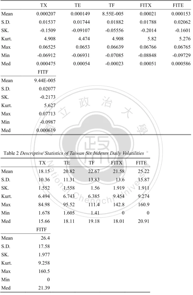
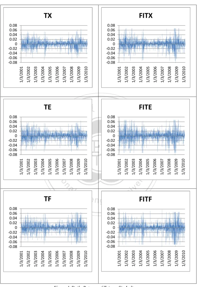
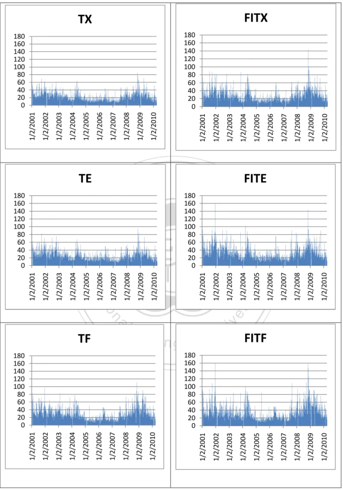
(10) The underlying data are daily closing price of stock and future market indexes, January 2001~March 2010, taken from TEJ Database. I calculate daily returns as the change in log price, day to day. I provide a variety of descriptive statistics for returns in Table 1 and plot the six indices’ returns in Figure 1. We can see that the Finance Sector Index and it’s future has relative lower mean returns than the other indices. All the six indices have dramatically returns fluctuation around 2002~2004 and 2007~2009.. Following Alizadeh, Brandt and Diebold (2002), we estimate daily variance. 政治大. using daily high and low prices. For market i on day t, σ =0.361 ln P. 學. Because σ. 立. ,. is the highest price in market i on day t, and P is the daily lowest price.. ‧ 國. where P. − ln P. is an estimator of the daily variance, the corresponding estimate of the. ‧. annualized daily percent standard deviation (volatility) is σ =100 365 × σ. . The. Nat. sit. y. formula here using 365 days instead of 240 days (actually trading days in a year) is. n. al. er. io. the same with Diebold and Yilmaz’s approach and will not affect our outcome. I. i Un. v. provide descriptive statistics for volatilities in Table 2 and give the plot in Figure 2.. Ch. engchi. We find that FITF has the highest mean and standard deviation. It means that FITF has greater daily volatility in the past 10 years, especially from 2007 to 2009.. [Insert Table 1, Table 2, Figure 1and Figure 2 Here] 3.1 Full-sample analysis. Here I provide a full-sample analysis of Taiwan six key index classes return and volatility spillovers. I begin by characterizing return and volatility spillovers over 6.

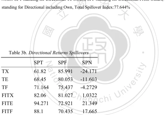
(11) the entire sample, January 2001~March 2010. Later I will track time variation in spillovers via rolling sample estimation. Before I test for generalized VAR model, it is necessary to do the unit root tests of each variable. The result from Augmented Dickey-Fuller Unit Root Test shows that all the variables are stationary at their levels. In the following empirical work, I use first-order generalized VAR with 10-step-ahead forecasts.2 I report Spillover Indexes for returns and volatility in Tables 3 and 4, respectively.. [Insert Table 3 and Table 4 Here]. The xy. 政治大 entry in the 立spillover table is the estimated contribution to the. ‧ 國. 學. forecast error variance of index x coming from shocks to index y. The off-diagonal column sums represent directional to others and the off-diagonal row sums represent. ‧. directional from others. The total spillover rate, which appears in the lower right. Nat. sit. y. corner of the table, is approximately the off-diagonal column (or row) sums relative to. n. al. er. io. the column (or row) sums including diagonals. The spillover table shows a “to and. i Un. from” two-way decomposition of the total spillover effect.. Ch. engchi. v. In Table 3, we can see that gross directional returns spillovers to others from the future markets are relatively large (especially FITE), at 82.06 percent, 94.27 percent and 88.10 percent, respectively. From the “directional from others” column, gross directional return spillovers from others to TX is relatively large, at 85.99 percent. In Table 4, we can also see that gross directional volatility spillovers to others from the future markets are relatively large (especially FITF), at 84.60 percent, 102.03. 2. The method is the same with Diebold and Yilmaz’s approach and it will not affect our key conclusions. 7.

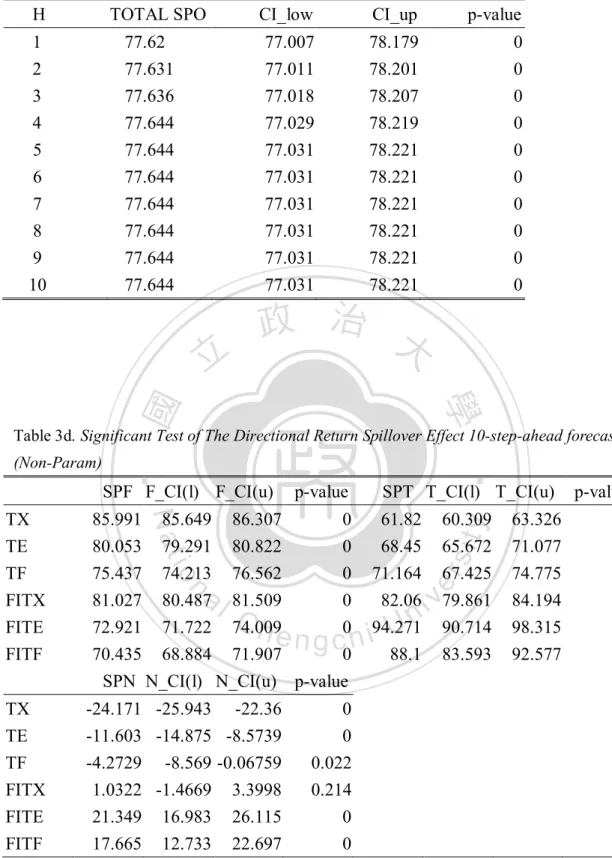
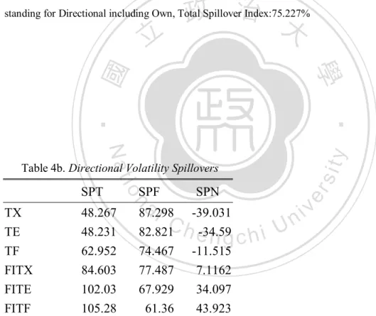
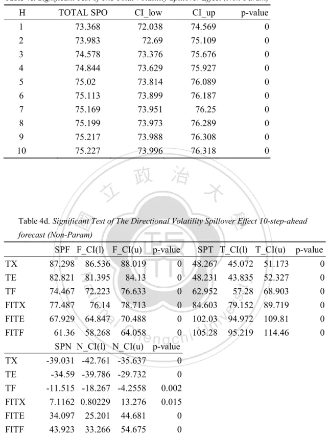
(12) percent and 105.28 percent, respectively. The spillovers here exceed 100 percent is mainly because we standardize the formulae for row sums (directional from others) and the sum of “directional to others” column must equal the sum of “directional from others” column. From the “directional from others” column, gross directional volatility spillovers from others to TX is relatively large, at 87.30 percent. Considering net directional returns and volatility spillovers, future markets have positive and spot markets have negative net spillovers. As for net directional return spillovers, the largest SPT and SPF are to others from FITE and from others to TX. As for net directional volatility spillovers, the largest SPT and SPF are to others from. 治政大 in both returns and FITF and from others to TX. The total spillovers are important 立 volatilities since almost 75% of forecast error variance comes from spillovers, both ‧ 國. 學. for returns (78%) and volatilities (75%).. ‧. sit. y. Nat. Here I use the nonparametric bootstrapping method (Efron, 1979) to conduct. io. er. the significant test. By simulating 1000 replications, I calculate the 95% confidence. al. interval and check the p-value of the directional spillover 10-ahead forecast. In table 3,. n. iv n C SPF and SPT are all statistically significant. NET spillovers, except FITX h e n gConsidering chi U is insignificant, all others are statistically significant. In Table 4, SPF, SPT and SPN are all statistically significant.. 3.2 rolling-sample analysis The full-sample Spillover Tables and Spillover Indexes provide a useful summary of average behavior, but they are likely to miss the potentially cyclical movements in spillovers. To address this issue, I estimate the models using 100 days 8.

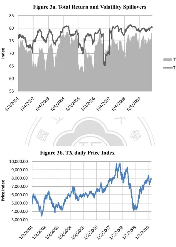
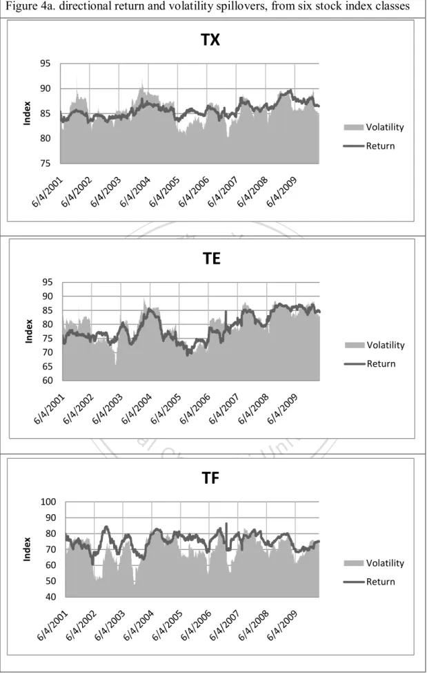
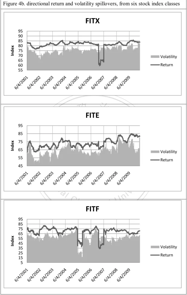
(13) rolling samples. I present the Spillover Plot for returns and volatility in Figure 3. [Insert Figure 3 Here] The total return spillover plot usually fluctuates between seventy-five and eighty percent, occasionally falling below seventy-five percent. The total volatility spillover plot usually fluctuates between seventy and eighty percent, occasionally falling below seventy percent. The total volatility spillover plot (TVS) and the total return spillover plot (TRS) display similar trend pattern, but TVS ranges widely than TRS. At the beginning of 2007, the total return spillovers and the total volatility. 政治大. spillovers both dropped to around sixty-five percent (the relative lower rate in the. 立. decade). Soon after the falling, they climbed up dramatically to about eighty percent. ‧ 國. 學. (the relative higher rate in the decade) and then the global financial crisis occurred, lasting from 2007~2009. During this period, the total return spillovers maintained. ‧. around eighty percent. The total volatility spillovers also came to the highest level. y. Nat. n. er. io. al. sit. (over seventy-five percent).. 3.3 rolling-sample directional spillover. Ch. engchi. i Un. v. After discussing the total dynamic spillover plot, we now also want to estimate the row and column dynamically. We call these directional spillover plots. In Figure 4, I present the directional return and volatility spillovers from the six stock index classes. The fluctuation of TX, TE and TF is about ten percent, twenty percent and thirty percent. The fluctuation of FITX, FITE and FITF is about twenty percent, forty percent and sixty percent. The plots show that the directional return and volatility spillover lines of all six indices vary obviously over time and FITF fluctuates larger than other indices. In Figure 5, I present the directional return and volatility spillovers 9.

(14) to the six stock index classes. Comparing with the directional spillovers from others, the spillovers to others vary greatly over time. We can find the Finance Sector Indices (TF and FITF) have an increasing trend. This can be easily figured out because there was a global financial crisis during 2007~2009 and MOU agenda between Taiwan and Mainland China governments during 2009~2010. [Insert Figure 4 and Figure 5 Here] Calculating difference between the “Contribution from” column sum and the “Contribution to” row sum, we can derive the net directional spillovers moving. 政治大. pattern. Figure 6 shows the net directional spillover plot. Overall, there has been very. 立. little net return and volatility transmission from the spot markets. This result is quite. ‧ 國. 學. easy to understand owing to stock index futures having the function on forecasting stock index and helping to transfer stock index returns risk. But we can still observe. ‧. net return spillovers from TE index to others reach about twenty percent during. y. Nat. io. sit. 2005~mid 2006. Net return spillovers from TF index to others reach about fifty. n. al. er. percent during 2009 and the first half of 2004. Further, net return and volatility. Ch. i Un. v. spillovers from FITE and FITF appear the most consistently positive and large.. engchi. Although FITX is a future index, it is not an important net transmitter of return and volatility. This is because FITE and FITF also influence FITX a lot.3 Following the financial market turmoil associating with the subprime mortgage market that started in July-August, 2007, net return spillover plot of FITF had an upward trend, and net return spillover plot of FITE had a downward trend. We can say that during the global financial crisis 2007~2009, net return and volatility spillovers from FITF affected mostly the other index. 3. The two major components of Taiwan stock market are Electronic sector and Finance sector. 10.

(15) [Insert Figure 6 Here]. 4. Conclusion In this paper I examine daily return and volatility spillovers of Taiwan spot and futures stock indices by using a generalized vector autoregressive model where forecast-error variance decompositions are invariant to variable ordering. I also calculate both gross and net directional return/volatility spillovers and look further in dynamic analysis. The result of empirical analysis can be summarized as follows: The clear channels of directional return/volatility spillovers to others are from FITE and. 治政大than trading volume of FITE FITF. Although trading volume of FITX are much larger 立 and FITF in Taiwan futures market, FITE and FITF are mainly traded by Institutional ‧ 國. 學. investors such as Securities Investment Trust, Foreign investors and Securities. ‧. Dealers. These Institutional investors are more professional and have more market. sit. y. Nat. information. That is why the return and volatility spillovers from FITE and FITF to. io. er. other indices are relatively large. Considering net directional returns and volatility. al. spillovers, future markets have positive and spot markets have negative net spillovers.. n. iv n C However, in rolling sample analysis, observe net return spillovers from h we e ncangstill chi U TE index to others reach about twenty percent during 2005~mid 2006. Net return. spillovers from TF index to others reach about fifty percent during 2009 and the first half of 2004. The above empirical findings reveal that the future markets play a dominant role in the return and volatility spillover to spot markets but we could not ignore return spillovers from spot to futures. Since the occurrence of the global financial crisis from 2007 and the MOU issue negotiated between Taiwan and Mainland China governments during 2009~2010, the Finance sector has a greater influence over Taiwan stock markets than Electronic sector in recent years. 11.

(16) References Tse, Y. (1999), ‘Price discovery and volatility spillovers in the DJIA index and futures markets’,Journal of Future Markets 29, P: 911-930. Bhar, R. (2001) Return and volatility dynamics in the spot and futures markets in Australian: An Intervention Analysis in a bivariate EGARCH-X framework. Journal of Futures markets, 21, 833-850. Meneu, V. & Torro., H.(2003) Asymmetric covariance in spot-futures markets. Journal of Futures Markets, 23, 1019-1046. Fu, L.Q. and Qing, Z.J. (2006), ‘Price discovery and volatility spillovers: Evidence from Chinese spot-futures markets’. Gupta, K. and Belwinder, S. (2006), ‘Price discovery and causality in spot and future markets in India’, The ICFAI Journal of Derivatives. Diebold, F.X. and Yilmaz, K. (2009), "Measuring Financial Asset Return and Volatility Spillovers, With Application to Global Equity Markets," Economic. 立. 政治大. ‧. ‧ 國. 學. Journal, 119, 158-171. Diebold, F.X. and Yilmaz, K. (2009), "Better to Give than to Receive: Predictive Directional Measurement of Volatility Spillovers," International Journal of Forecasting, forthcoming. (With discussion.) Forbes, K., Rigobon, R. (2002), ‘No Contagion, only Interdependence: Measuring Stock Market Comovements’, Journal of Finance, 57, 2223-2261. Karolyi, G.A. (1995), ‘A Multivariate GARCH Model of International Transmissions of Stock Returns and Volatility: The case of the United States and Canada’, Journal of Business and Economic Statistics, 13, 11-25. King, Mervyn A and Wadhwani, Sushil, (1990). "Transmission of Volatility between Stock Markets," Review of Financial Studies, Oxford University Press for Society for Financial Studies, vol. 3(1), pages 5-33. Koop, G., Pesaran, M.H., and Potter, S.M. (1996), “Impulse Response Analysis in Non-Linear Multivariate Models,” Journal of Econometrics, 74, 119–147. Pesaran, M.H. and Shin, Y. (1998), “Generalized Impulse Response Analysis in Linear Multivariate Models,” Economics Letters, 58, 17-29. Cho.Bauer(2002), “The analysis of Stock return change to Asian Equity Markets from US”,The Korean Journal of Financial Management, Vol.19, No.2, pp.181-200 Morana, C., Beltratti, A. (2006), ‘Comovements in International Stock Markets’, Journal of International Financial Markets, Institutions and Money Miyakoshi T(2003), "Spillovers of Stock Return Volatility to Asian Equity Markets from Japan and the US", Journal of International Financial Markets, Institutions & Money, No.13. pp.383-399. n. er. io. sit. y. Nat. al. Ch. engchi. 12. i Un. v.

(17) Table 1 Descriptive Statistics of Taiwan Six Indices Daily Returns TX. TE. TF. FITX. FITE. Mean. 0.000207. 0.000149. 8.55E-005. 0.00021. 0.000153. S.D.. 0.01537. 0.01744. 0.01882. 0.01788. 0.02062. SK.. -0.1509. -0.09107. -0.05556. -0.2014. -0.1601. Kurt.. 4.908. 4.474. 4.908. 5.82. 5.276. Max. 0.06525. 0.0653. 0.06639. 0.06766. 0.06765. Min. -0.06912. -0.06931. -0.07085. -0.08848. -0.09729. Med. 0.000475. 0.00054. -0.00023. 0.00051. 0.000586. FITF Mean. 9.44E-005. S.D.. 0.02077. SK.. -0.2173. Max. 0.07713. Min. -0.0987. Med. 0.000619. 立. 政治大. ‧. ‧ 國. 5.627. 學. Kurt.. Table 2 Descriptive Statistics of Taiwan Six Indexes Daily Volatilities. 18.15. 20.82. 22.67. 21.58. S.D.. 10.36. 11.31. 13.83. 13.6. SK.. 1.552. 1.56. 1.919. Kurt.. 6.494. Max. 84.98. 95.52. Min. 1.678. Med. 15.66. io. n. 9.454 e6.385 ngchi U. 26.4. S.D.. 17.58. SK.. 1.977. Kurt.. 9.258. Max. 160.5. Min. 0. Med. 21.39. 25.22 15.87. v 1.911 i n 9.274. 111.4. 142.8. 160.9. 1.605. 1.41. 0. 0. 18.11. 19.18. 18.01. 20.91. FITF Mean. FITE. y. Mean. a1.558 l C 6.743 h. FITX. sit. TF. er. TE. Nat. TX. 13.

(18) 14. i Un. s 1/3/2004 ity 1/3/2005. 1/3/2003. 0.06 0.04 0.02 0 -0.02 -0.04 -0.06 -0.08. Figure 1 Daily Returns of Taiwan Six Indices 1/3/2007 1/3/2008 1/3/2009 1/3/2010. 1/3/2008 1/3/2009 1/3/2010. 1/3/2008. 1/3/2009. 1/3/2010. 1/3/2005. 1/3/2004. 1/3/2003. 1/3/2002. 1/3/2001. 1/3/2010. 1/3/2009. 1/3/2008. 1/3/2007. 1/3/2006. 1/3/2005. 1/3/2004. 1/3/2003. 1/3/2002. 1/3/2007. 0.08 0.06 0.04 0.02 0 -0.02 -0.04 -0.06 -0.08. 1/3/2007. FITF. 1/3/2006. v 1/3/2006. FITE. 1/3/2006. 1/3/2005. er. 1/3/2002. 1/3/2001. 1/3/2010. 政治大 0.08. 1/3/2004. 0.08 0.06 0.04 0.02 0 -0.02 -0.04 -0.06 -0.08. 1/3/2003. engchi. 1/3/2002. Ch. 1/3/2001. TF 1/3/2009. 1/3/2008. 1/3/2007. 1/3/2005. ‧ 國 1/3/2006. 1/3/2004. 立. 1/3/2010. al. 1/3/2009. 1/3/2008. 1/3/2007. 1/3/2006. 1/3/2005. 1/3/2004. 1/3/2003. TE. ‧. n. 1/3/2003. 1/3/2002. 1/3/2001. 0.08 0.06 0.04 0.02 0 -0.02 -0.04 -0.06 -0.08. 學. io. 1/3/2002. 1/3/2001. 0.08 0.06 0.04 0.02 0 -0.02 -0.04 -0.06 -0.08. Nat. 1/3/2001. TX FITX. 0.08 0.06 0.04 0.02 0 -0.02 -0.04 -0.06 -0.08.

(19) 15. Figure 2 Daily Volatilities of Taiwan Six Indices 1/2/2009 1/2/2010. 1/2/2009. 1/2/2010. 1/2/2006. 1/2/2008. 180 160 140 120 100 80 60 40 20 0. 1/2/2008. FITF 1/2/2007. v. 1/2/2007. 1/2/2006. i Un. s1/2/2004 ity 1/2/2005. 1/2/2003. 140 120 100 80 60 40 20 0. 1/2/2005. er. 1/2/2002. 1/2/2001. 政治大 180 160. 1/2/2004. 180 160 140 120 100 80 60 40 20 0. 1/2/2003. engchi. 1/2/2002. Ch. 1/2/2001. 1/2/2010. 1/2/2009. 1/2/2008. 1/2/2007. ‧ 國 1/2/2006. 1/2/2005. 1/2/2004. 立. 1/2/2010. al. 1/2/2009. TF. 1/2/2008. 1/2/2007. 1/2/2006. 1/2/2005. 1/2/2004. 1/2/2003. TE. ‧. n. 1/2/2003. 1/2/2002. 1/2/2010. 1/2/2009. 1/2/2008. 1/2/2007. 1/2/2006. 1/2/2005. 1/2/2004. 1/2/2003. 1/2/2002. 1/2/2001. 1/2/2010. 1/2/2009. 1/2/2008. 1/2/2007. 1/2/2006. 1/2/2005. 1/2/2004. 1/2/2003. 1/2/2002. 1/2/2001. 180 160 140 120 100 80 60 40 20 0. 學. io. 1/2/2002. 1/2/2001. 180 160 140 120 100 80 60 40 20 0. Nat. 1/2/2001. TX FITX. 180 160 140 120 100 80 60 40 20 0. FITE.

(20) Table 3a. Return Spillover Table, Six Index Classes. ============================================================= TX TE TF FITX FITE FITF SPF TX TE TF FITX FITE FITF. 14.009 14.07 11.451 12.869 12.796 10.634. 16.377 19.947 9.7472 15.11 17.894 9.3215. 14.669 10.766 24.563 13.623 10.181 21.924. 17.307 17.481 14.27 18.973 18.285 14.718. 20.738 24.977 12.748 21.97 27.079 13.838. 16.898 12.76 27.221 17.456 13.765 29.565. 85.991 80.053 75.437 81.027 72.921 70.435. SPT. 61.82. 68.45. 71.164. 82.06. 94.271. 88.1. 465.86. Inc Own 75.829 88.397 95.727 101.03 121.35 117.67 77.644 ============================================================= Notes: SPT standing for Directional To Others, SPF standing for Directional From Others, Inc Own. 政治大. standing for Directional including Own, Total Spillover Index:77.644%. 立. ‧. ‧ 國. 學. Table 3b. Directional Returns Spillovers. Ch. engchi. Notes: SPN standing for Net Directional Returns Spillovers. 16. sit er. al. -24.171 -11.603 -4.2729 1.0322 21.349 17.665. y. SPN. 85.991 80.053 75.437 81.027 72.921 70.435. n. 61.82 68.45 71.164 82.06 94.271 88.1. SPF. io. TX TE TF FITX FITE FITF. Nat. SPT. i Un. v.

(21) Table 3c. Significant Test of The Total Return Spillover Effect (Non-Param). H. TOTAL SPO. 1 2 3 4 5 6 7 8 9 10. 77.62 77.631 77.636 77.644 77.644 77.644 77.644 77.644 77.644 77.644. 立. CI_low. CI_up. p-value. 77.007 77.011 77.018 77.029 77.031 77.031 77.031 77.031 77.031 77.031. 78.179 78.201 78.207 78.219 78.221 78.221 78.221 78.221 78.221 78.221. 0 0 0 0 0 0 0 0 0 0. 政治大. ‧ 國. 學. Table 3d. Significant Test of The Directional Return Spillover Effect 10-step-ahead forecast. n. al. Ch. SPT T_CI(l) T_CI(u). engchi. -24.171 -25.943 -22.36 -11.603 -14.875 -8.5739 -4.2729 -8.569 -0.06759 1.0322 -1.4669 3.3998 21.349 16.983 26.115 17.665 12.733 22.697. 0 0 0.022 0.214 0 0. 17. 60.309 65.672 67.425 79.861 90.714 83.593. y. 61.82 68.45 71.164 82.06 94.271 88.1. sit. 85.991 85.649 86.307 0 80.053 79.291 80.822 0 75.437 74.213 76.562 0 81.027 80.487 81.509 0 72.921 71.722 74.009 0 70.435 68.884 71.907 0 SPN N_CI(l) N_CI(u) p-value. io. TX TE TF FITX FITE FITF. Nat. TX TE TF FITX FITE FITF. p-value. er. SPF F_CI(l) F_CI(u). ‧. (Non-Param). i Un. v. 63.326 71.077 74.775 84.194 98.315 92.577. p-value 0 0 0 0 0 0.

(22) Table 4a. Volatility Spillover Table, Six Index Classes. ============================================================= TX TE TF FITX FITE FITF SPF TX TE TF FITX FITE FITF. 12.702 12.479 8.6345 10.256 9.5968 7.3013. 13.042 17.179 6.8413 10.404 12.097 5.8454. 13.621 10.172 25.533 11.323 9.1188 18.717. 18.814 18.416 13.44 22.513 19.415 14.518. 22.256 26.845 13.534 24.412 32.071 14.978. 19.565 14.909 32.016 21.092 17.701 38.64. 87.298 82.821 74.467 77.487 67.929 61.36. SPT. 48.267. 48.231. 62.952. 84.603. 102.03. 105.28. 451.36. Inc Own 60.969 65.41 88.485 107.12 134.1 143.92 75.227 ============================================================= Notes: SPT standing for Directional To Others, SPF standing for Directional From Others, Inc Own. 政治大. standing for Directional including Own, Total Spillover Index:75.227%. 立. ‧. ‧ 國. 學. io. SPT. SPF. SPN. al 87.298 -39.031 iv n C 82.821 h e -34.59 ngchi U. n. TX TE TF FITX FITE FITF. 48.267 48.231 62.952 84.603 102.03 105.28. er. sit. y. Nat. Table 4b. Directional Volatility Spillovers. 74.467 77.487 67.929 61.36. -11.515 7.1162 34.097 43.923. Notes: SPN standing for Net Directional Returns Spillovers. 18.

(23) Table 4c. Significant Test of The Total Volatility Spillover Effect (Non-Param). H. TOTAL SPO. 1 2 3 4 5 6 7 8 9 10. 73.368 73.983 74.578 74.844 75.02 75.113 75.169 75.199 75.217 75.227. 立. CI_low. CI_up. p-value. 72.038 72.69 73.376 73.629 73.814 73.899 73.951 73.973 73.988 73.996. 74.569 75.109 75.676 75.927 76.089 76.187 76.25 76.289 76.308 76.318. 0 0 0 0 0 0 0 0 0 0. 政治大. ‧ 國. 學. Table 4d. Significant Test of The Directional Volatility Spillover Effect 10-step-ahead forecast (Non-Param). n. al. -39.031 -34.59 -11.515 7.1162 34.097 43.923. Ch. SPT T_CI(l) T_CI(u). engchi. -42.761 -35.637 -39.786 -29.732 -18.267 -4.2558 0.80229 13.276 25.201 44.681 33.266 54.675. 0 0 0.002 0.015 0 0. 19. y. 45.072 43.835 57.28 79.152 94.972 95.219. sit. 48.267 48.231 62.952 84.603 102.03 105.28. er. io. TX TE TF FITX FITE FITF. 87.298 86.536 88.019 0 82.821 81.395 84.13 0 74.467 72.223 76.633 0 77.487 76.14 78.713 0 67.929 64.847 70.488 0 61.36 58.268 64.058 0 SPN N_CI(l) N_CI(u) p-value. Nat. TX TE TF FITX FITE FITF. p-value. ‧. SPF F_CI(l) F_CI(u). i Un. v. 51.173 52.327 68.903 89.719 109.81 114.46. p-value 0 0 0 0 0 0.

(24) Figure 3a. Total Return and Volatility Spillovers 85 80. Index. 75 70 TVS 65. TRS. 60 55. 立. 政治大. ‧ 國. 學. 7,000.00. 5,000.00 4,000.00. y. sit. al. n. 6,000.00. io. Price Index. 8,000.00. Nat. 9,000.00. er. 10,000.00. ‧. Figure 3b. TX daily Price Index. Ch. engchi. 3,000.00. 20. i Un. v.

(25) Figure 4a. directional return and volatility spillovers, from six stock index classes. TX 95. Index. 90 85 Volatility 80. Return. 立. ‧ 國. ‧. Volatility Return. n. al. er. io. sit. y. Nat. 95 90 85 80 75 70 65 60. 政 TE 治大. 學. Index. 75. Ch. engchi. i Un. v. TF. 100. Index. 90 80 70 60. Volatility. 50. Return. 40. 21.

(26) Figure 4b. directional return and volatility spillovers, from six stock index classes. 95 90 85 80 75 70 65 60 55. Volatility Return. 立. 95. io. al. n. Index. Return. y. Nat. 45. Volatility. sit. 55. ‧. 65. ‧ 國. Index. 75. 學. 85. 政FITE治大. er. Index. FITX. Ch. engchi FITF. 95 85 75 65 55 45 35 25 15 5. i Un. v. Volatility Return. 22.

(27) Figure 5a. directional return and volatility spillovers, to six stock index classes. TX 100. Index. 80 60 40. Volatility. 20. Return. 立. ‧ 國. ‧. Volatility Return. n. al. er. io. sit. y. Nat. 120 100 80 60 40 20 0. 政治大 TE. 學. Index. 0. Ch. engchi. i Un. v. Index. TF. 140 120 100 80 60 40 20 0. Volatility Return. 23.

(28) Figure 5b. directional return and volatility spillovers, to six stock index classes. 120 110 100 90 80 70 60 50 40. Return. 立. 政FITE治大. ‧ 國. ‧. Volatility Return. n. al. er. io. sit. y. Nat. 170 150 130 110 90 70 50 30. Volatility. 學. Index. Index. FITX. Ch. engchi. i Un. v. Index. FITF. 170 150 130 110 90 70 50 30. Volatility Return. 24.

(29) Figure 6a. net directional return and volatility spillovers, six stock index classes. 80 60 40 20 0 -20 -40 -60 -80. Return. 政治大 TE. 立. ‧. ‧ 國. 2005~mid2006. sit. al. n. Index. Return. er. io. 80 60 40 20 0 -20 -40 -60 -80. Volatility. y. Nat. 80 60 40 20 0 -20 -40 -60 -80. Volatility. 學. Index. Index. TX. Ch. first half of 2004. engchi. i Un. v. TF. 2009. Volatility Return. 25.

(30) Figure 6b. net directional return and volatility spillovers, six stock index classes. 80 60 40 20 0 -20 -40 -60 -80. Return. 立. 政治大 FITE. ‧ 國. ‧. Volatility Return. n. al. er. io. sit. y. Nat. 80 60 40 20 0 -20 -40 -60 -80. Volatility. 學. Index. Index. FITX. Ch. engchi. i Un. v. Index. FITF. 80 60 40 20 0 -20 -40 -60 -80. Volatility Return. 26.

(31)