早期視覺下之生物啟發式混合質感邊界偵測模型

(1)

國立交通大學

電機與控制工程學系

碩士論文

早期視覺下之生物啟發式混合質感邊界偵測模型

Biological-Inspired Model for Hybrid-Order

Texture Boundary Detection during Early Vision

研究生：林愷翔

指導教授：林進燈博士

(2)

早期視覺下之生物啟發式混合質感邊界偵測模型

學生：林愷翔

指導教授：林進燈博士

國立交通大學電機與控制工程研究所

中文摘要

本論文提出一個由生物觀點啟發的多通道質感邊緣偵測演算法用以偵測不同質感間的邊界。此演算法用高斯濾波器抽取質感的一階特徵，另外使用一組不同參數的 GABOR 濾波器抽取二階特徵。這些不同的特徵接著被予以整合形成一個 N 維的特徵空間。我們會分別計算每一個像素點(pixel)和他相鄰點在特徵空間中的差異，在消除調差異小的像素點之後，我們可以得到一個粗的邊界影像。最後我們使用區域頂點偵測的方式，找出精確邊界的位置。此演算法簡單並且直觀，因此可實現於仿細胞神經網路(Cellular Neural Networks; CNN)。CNN 擁有一些重要的特性，例如有效率的及時運算能力及方便於大型積體電路(VLSI)的實現。在論文裡，我們大量測試我們的演算法在合成的質感影像上，而這些質感都是隨機從“Brodatz texture＂中取出來的。由實驗結果我們可以發現均勻質感的邊界都可成功而精確的找出，而對於不規則或不均勻的質感，演算法仍會找出一些符合我們人眼感受的特性。

(3)

Biological-Inspired Model for Hybrid-Order

Texture Boundary Detection during Early Vision

Student: Kai-Hsiang Lin Advisor: Dr. Chin-Teng Lin

Department of Electrical and Control Engineering National Chiao-Tung University

Abstract

In this thesis a multi-channel texture boundary detection technique inspired

from human vision system is presented. This algorithm extracts 1st-order features by a Gaussian filter and 2nd –order features by a set of even-symmetric Gabor filters. The hybrid-order features are integrated to construct an N-dimensional feature space.

The difference between each pixel with its neighbors is measured in feature space,

and coarse boundaries are obtained after eliminate pixels with small difference.

After obtaining coarse boundaries, we use local peak detection to get the precise

boundaries.

The proposed algorithm is simple and straight-forward such that it can be

implemented on Cellular Neural Networks (CNN) which possesses some important

characteristics such as efficient real-time processing capability and feasible very

large-scale integration (VLSI) implementation.

We also extensively tested our algorithm on synthetic textures randomly picked

from “Brodatz texture”, and from experiments it can be found that boundaries of

uniform textures are detected successfully and have high spatial-accuracy. For the

textures that are non-uniform or non-regular, the results also reflect some

(4)

誌謝

在電控所這兩年以來，首先要感謝林進燈博士提供我一個理想的研究環境，同時在學業上與求學態度上給予啟蒙與悉心指導，使得本論文能順利完成。另外特別地要感謝交大應藝所陳一平教授的幫助與教導，使得我可以順利解決研究方面的問題。同時也要感謝實驗室鶴章學長、仁峰學長、俊隆、聖哲、群立、朝暉、世茂、宇文、剛維、盈彰、弘昕及宗恆給予我鼓勵與快樂。最後，謹以此論文獻給我最愛的家人，感謝爸媽以及妹妹的支持，讓我能夠專心於課業上的研究，順利完成學業。還有感謝婷俞不停地幫我加油打氣，讓我能夠鼓起勇氣完成研究。非常感謝你們！

(5)

List of Tables

(8)

List of Figures

Fig. 1-1 (a) preattentively discriminable pattern; (b)not preattentively discriminable pattern...3 Fig. 2-1: visual pathway of human brain(adapted from sensation and

perception p.38p.39)...10 Fig. 2-2 a schematic diagram of receptive field of bipolar cells ...11 Fig. 2-3 DoG function in spatial and frequency domain ...11 Fig. 2-4 an schematic diagram about receptive field from ganglion cell to

V1 cells ...12 Fig. 2-5 schematic diagram of cortex functional module ...13 Fig. 2-6 a schematic diagram of FIT ...15 Fig. 2-7 an example to illustrate the effect of pop-out (a)no pup-out effect;

(b) pop-out effect exists...16 Fig. 2-8 Typical results of a visual search experiment: (a) the result when

pop-out occurs; (b) the result when there is no pop-out. ...16 Fig. 2-9 (a) element with different orientations; (b) elements with the

same orientations(adapted from sensation and perception p.164)...17 Fig. 3-1 Simplified block diagram for hybrid-order boundary detection ..19 Fig. 3-2 detailed block diagram for hybrid-order boundary detection

algorithm...20 Fig.3-3 an example demonstrating coarse boundary detected by 1st-order

feature (a) input image; (b) boundaries detected...22 Fig. 3-4 An example demonstrating the effect of 1st-order feature in

boundary detection: (a) 150×300 image (D101-D102); (b)boundary detected by 2nd-order feature; (c)boundary detected by 1st-order

feature ...23 Fig. 3-5 An example of 2D Gabor type filtering. (a) is a standard 2D

Gabor type filter in time domain, and (b) is in frequency domain. ...25 Fig. 3-6 an example demonstrates the effect of rectifying (a) input; (b)

output without rectifying; (c) output with rectifying...27 Fig. 3-7 (a) input; (b) output before rectification; (c) output after

rectification ...28 Fig. 3-8 an schematic diagram of an 3-dimensional feature space...29 Fig. 3-9 frequency response of (a) Gabor filters in different orientation (b) Gabor filters in different frequency band...31 Fig. 3-10 (a)input (b)coarse boundary (c)3D version of (b) (d)(c)after

(9)

peak detection (d)superposition of (a) and (d) ...34 Fig. 4-1 feature image of band 1(a)0° (b)45° (c)90°_(d) 135°_{(e) coarse}

boundaries (d) (e) after peak detection ...40 Fig. 4-2 feature image of band 2 (a)0° (b)45° (c)90°_(d) 135°_{(e) coarse}

boundaries (d) (e) after peak detection ...43 Fig. 4-5 (c) coarse boundaries (d) (c) after boundary detection (e)

superposition of (d) and input...43 Fig. 4-6 (a)coarse boundaries detected by 1st-order features (b)(a)after

detection (c)coarse boundaries detected by 2nd-order features (d)(c)after detection (e)coarse boundaries detected by hybrid-order features (f) (f)after detection (g)superposition of (f) and input ...46 Fig. 4-7 (a) coarse boundaries without log transform; (b)(a) after log

transform; (c)(a)after thresholding; (d)(b) after thresholding; (e)2D version of (c); (f) 2D version of (d); (g)(f) after peak detection;

(h)superposition of input and (h)...49 Fig. 4-8 an example of error estimation (a) input; (b) answer(middle line); (c) output; ...64 Fig. 4-9 histogram of error estimation ...65 Fig. 4-10 an example of test image with big estimation errors(D50D32); (a) input; (b) output;...66 Fig. 4-11 an example of test image with big estimation errors(D105D83);

(a) input; (b) output;...66 Fig. 4-12 an example of test image with big estimation errors(D17D70); (a) input; (b) output;...66 Fig. 4-13 an example of test image with big estimation errors(D8D16); (a)

(10)

Chapter 1 Introduction

1.1 Motivation

Boundary detection is an important and fundamental topic in image processing, and the output of an image segmentation can applied in many applications, such as tracking, stereo, pattern recognition... etc. Boundary detection basically is a partitioning of an image into related sections or regions, and finding the boundaries. This process seems intuitive in human vision, but it is hard to do this job automatically in computer vision.

The human visual system is able to effortlessly integrate local features to form our rich perception of patterns, despite the fact that visual information is discretely sampled by the retina and cortex. It seems clear, both from biological and computational evidence, that some form of data compression occurs at a very early stage in image processing. Moreover, there is much physiological evidence suggesting that one form of this compression involves finding boundaries and other information-high features in images.

In this thesis we will propose a simple model which mimics the early stage of human vision which integrate hybrid-order features unsupervisedly, and it should be able to be implemented on circuit of CNN.

1.2 State of Problems

Early vision, also known as preattentive vision, includes those mechanisms that subserve the first stages of visual processing. These mechanisms can operate in parallel across the visual field, and is believed to be used for detecting the most basic visual features, such as color, luminance, orientation, motion etc.

The most fundamental feature we use in human vision is the difference of light intensity that reflects into our eyes. In the retina level, our eyes are just like a band pass filter, and grab the information where intensity changes abruptly. We sometimes

(11)

call the position of these changes 1st-order boundaries, and the first order features can be generally equal to the mean of a local area. Some boundary detection algorithms based on this feature are zero crossing of the Laplacian of the Gaussian and Canny’s boundary detector [1]. There is a common problem in computer vision that they do not make a distinction between contours of objects which are the actual primitives needed in most application. It reveals that there are still some other mechanisms during visual perception, and in this thesis we focus on texture segregation.

For texture analysis, an important finding in the physiology and psychophysics of the visual system of monkeys and cats, made in the beginning of the 1960s was that the majority of neurons in the primary visual cortex respond to a line or a boundary of a certain orientation in a given position of the visual field. In 1981, Hubel and Wiesel find two types of orientation-selective neuron, one that was sensitive to the of lines and boundaries, called simple cell, and another that was not, called complex cell [2], [3]. The receptive field of simple cell can be modeled by Gabor function, and it has been widely used to extract information which is called 2nd–order features hiding in texture. The mechanism of 2nd–order features is more commonly known as the filter- rectify-filter cascade. This consists of early linear filtering subunits, a no linearity (e.g., rectification), and a late linear filter.

There are various texture algorithms with performance evaluated against the performance of the human visual system doing the same task.

There are some observations from psychophysics help us form hypotheses about what image properties are important in human texture perception. For example, consider the texture pairs in Fig. 1-1(a) and Fig.1-1(b), first described by Julesz [4]. These two images both consist of two regions each of which is made up of different texture tokens. This fact is obvious in Fig.1-1(a), but in Fig.1-1(b) close scrutiny of the texture image is necessary to notice it. With immediate perception of Fig. 1-1(b), does not result in the perception of two different textured regions; instead only one uniformly textured region is perceived. Julesz says that texture pair in Fig.1-1(a) is “effortlessly discriminable” or “preattentively discriminable.”, and the texture pair in Fig.1-1(b) is not.

Here comes the question. If there is an algorithm which can detect the difference of the two texture patterns in Fig.1-1(b), the result of this algorithm is correct or not? This result may be correct if it is a special purpose algorithm designed to detect such scrutably different regions. On the other hand, this result is incorrect if it is to be a

(12)

computational model of how the human visual system processes texture. The algorithm proposed in this thesis belongs to the second case, and this property can help us roughly judge whether the results of the proposed algorithm are correct or not.

(a)

(b)

Fig. 1-1 (a) preattentively discriminable pattern; (b)not preattentively discriminable pattern

1.3 Related Works

1.3.1 Texture Analysis

“Definition” of Texture

At first, we should give a definition to texture, but it is unfortunately that there is not a precise and identical definition to texture until now. Although there is not a best definition to texture, this feature is so obvious that we still can’t neglect it. This situation is analogic to the tone in sound. We can easily distinguish the sound between violin and piano, but it is also hard to give a physical meaning to tone.

Many people have proposed some descriptions about texture, and the “definition” of texture is formulated depending on the particular application and that there is no generally agreed upon definition. We give some perceptually motivated examples here.

• “We may regard texture as what constitutes a macroscopic region. Its structure is simply attributed to the repetitive patterns in which elements or primitives are arranged according to a placement rule.” [5]

(13)

•

“A region in an image has a constant texture if a set of local statistics or other local properties of the picture function are constant, slowly varying, or approximately periodic.” [6]

• “The notion of texture appears to depend upon three ingredients: (i) some local‘order’ is repeated over a region which is large in comparison to the order’s size,(ii) the order consists in the nonrandom arrangement of elementary parts, and (iii)the parts are roughly uniform entities having approximately the same dimensions everywhere within the textured region.” [7]

In this thesis we refer to descriptions which have been proposed, and simplify the situation:

1. Texture is characterized by properties of a local region and in this region there should adequate spatial-relationships between elements or primitives. In this thesis spatial-relationships simply mean the orientation and frequency.

2. Here we discuss the homogeneous texture which means that there are similar features over all single texture patterns. In means that the size and orientation invariant problems which may not be discriminable are not considered in this thesis.

Filter Design

There have been many algorithms to cope with this topic, and these algorithms may generally be grouped into the following major classes: feature space clustering, statistical classification, multi-channel filtering approaches: texture gradient operators, optimal filtering technique, and toxton-based methods. Among the algorithms mentioned above, the multi-channel filtering approach appears to be one of successful one in texture segmentation. Here we will discuss some algorithms in this class.

Supervised methods

Bovic, Clark and Geisler [8], 錯誤! 找不到參照來源。 give a very detailed analysis of the Gabor function using localized spatial filters for texture feature extraction. Bovik mentioned three supervised approaches to select filter locations using empirical information based on the power spectrum characteristics of the individual textures. For strongly oriented textures, the most significant spectral peak

(14)

along the dominant orientation direction is used as a filter location. Picking the lower fundamental frequency identifies periodic textures. Finally, the non-oriented textures using the center frequencies of the two largest maxima are recommended. It is clear that an automated method is more attractive.

Dunn and Higgins [10] developed a method to select optimal filter parameters based on known samples of the textures. This is a totally supervised approach that focused mainly on using the minimum number of filters. Only the specific filter that separates two textures optimally is used to partition an image. The optimal filter responds strongly to one class and may express a lack of textural information of the other class. This other class is not identified to have a particular characteristic but lacking a characteristic of the other class. The more global solution to the problem is to spread filters throughout the frequency domain field to capture salient information.

Unsupervised methods

By providing near uniform coverage of the spatial-frequency domain with Gabor filters, the problem of selecting central frequencies is avoided. Jain and Farrokhnia [11] implemented real Gabor filters for texture segmentation using frequency bandwidth of one octave, center frequency spacing of one octave, angular bandwidth of 45°, and angular spacing of 45°.

The frequencies used in it for filters are:

2

1 , 2 2, 4 2, ……

(

Nc/4

)

2 Cycles /image width

For textures with distinct spectral peaks which correspond to some global regularities, T. N. Tan proposed a useful method [12] to design Gabor dilters automatically. The central step in the algorithm is spectral detection. It detects a global spectral peak a time, and repeatedly detects conspicuous peaks by erasing operation on the spatial frequency plane: the power spectrum of a small neighborhood (e.g. 7×7) around the detected peak is set to zero. The iteration of peak detection terminates when the ratio of the magnitude of current peak to that of the first (e.g., the highest) peak is less than a pre-specified value (e.g., 80%).

Feature Extraction

(15)

A number of feature extraction methods were proposed to extract useful information from the filter outputs. Clausi and Jernigan [13] reviewed some feature extraction methods. Some of which include:

1. Using the Magnitude Response, where the texture identification can be performed based on the magnitude of the output of the Gabor functions [8]. In the case of a filter that matches the particular texture the magnitude of the output is large to allow identification.

2. Applying the Spatial Smoothing where Gaussian smoothing is known to improve the performance of Gabor filters for texture analysis. Bovik et al [8] recommended post filtering the channel amplitudes with Gaussian filters having the same shape as the corresponding channel filters, but wider spatial extents.

3. Using only the Real Component Jain and Farrohknia [11] used a bank of even symmetric Gabor filters to characterize the channels.

4. Using Pixel Adjacency Information Jain and Farrokhnia suggested in [11] using this method as extra features due to the fact that pixels belonging to the same texture are close to each other, so they should be clustered together. However, this will not perform well if there are some texture regions that are not adjacent in the image.

5. Using a Non Linear Sigmoidal function that saturates the output of the filter where each filter image was subjected to a Sigmoidal non linear transformation [11] that can be interpreted as a blob detector. It is indicated by:

( )

_tt e e t tenh t _α α α ϕ 2₂ 1 1 − − + − = =

Where a is an empirical constant, a = 0.25. Their explanation was that most textures can be characterized by blobs of different sized and orientations. 6. Applying Full Wave Rectification: many HVS models consider the

evolvement of non linear behaviour [14]. Adding the absolute value of real and imaginary responses -full wave rectification- is a non linear method that is used to process the complex filter outputs [13].

(16)

1.3.2 Cellular Neural Networks

As we have mentioned above, there have been a lot of researches on texture based on the Gabor filter, but a drawback of Gabor filtering approaches is that they are computationally intensive.

Recently, a novel class of information-processing system called cellular neural networks (CNN) has been proposed [15], [16]. Cellular neural/nonlinear networks (CNN’s) show a strong resemblance to biological visual systems. It is therefore not surprising that several CNN models have been produced for the unraveling of the processing in some parts of the vertebrate visual pathway [18]

,

and the Gabor-like filters also have been implemented on CNN [20].

The advantage of CNN’s is that they can be implemented in analog VLSI alongside photosensors which sense the image, and the filter outputs can be computed in less time than required by serial digital computer implementations and be read off the chip directly, relieving the computational bottleneck of preprocessing with Gabor filters.

1.4 Research Scope

At present, there is no definitive model for dealing with first- and 2nd-order information, and in this thesis a structure is proposed trying to model this process. We focus on mimicking the Preattentive stage of visual perception, so there would be not any clustering or classification method. In order to overcome insufficiency of only considering single order feature, we integrate 1st and 2nd –order features simultaneously. The proposed algorithm is totally straight forward and simple, such that it can be implemented on CNN. In this thesis we focus on the designing algorithm, and the part of implementing the proposed algorithm on CNN would be in another thesis [19].

1.5 Thesis Organization

This thesis is organized as follows. Chapter 2 introduces knowledge form Physiology and Psychophysics about Vision. In Chapter 3 describes our hybrid-order texture boundary detection algorithm in detail. Chapter 4 shows the experimental

(17)

(18)

Chapter 2 Knowledge from Physiology and

Psychophysics about Vision

Human vision is a powerful and elaborate system which can extract features and integrate them effectively. From physiology and psychophysics there are evidences that human visual system makes such a difference in its early stages of visual information processing [21], [22]. The initial stages of this visual processing are very important in this respect as they detect and group various types of salient features, such as curvature, line orientation, color, frequency.

(19)

2.1 V1 Receptive Field on Cortex & Linear System

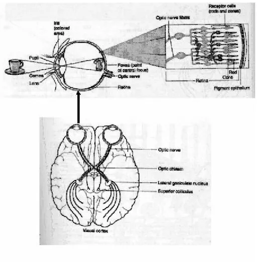
Fig. 2-1: visual pathway of human brain(adapted from sensation and perception p.38p.39)

As we can see in the Fig. 2-1, the retina is the first station in the visual sensation, where the absorption of the light is taking place in the photoreceptors, which is the beginning of the transformation of photo-quantum into electrical signals. These signals generated in the receptors travel through bipolar, horizontal, and amacrine cells to finally reach the ganglion cells, which then transmit these signals out of the back of the eye in the optic nerve. An important property of this network of retinal neurons is that signals from many receptors converge on to each ganglion cell. This convergence, combined with inhibition, which is mostly transmitted across the retinal by the horizontal and amacrine cells, and it can be modeled Fig. 2-2.

(20)

Fig. 2-2 a schematic diagram of receptive field of bipolar cells

We can formulate the overall response above by difference of Gaussian (DOG) function (see Fig. 2-3). The positive Gaussian which is thinner represents the contribution of photo receptors which directly link to bipolar cell. The negative Gaussian which is wider represents receptors which indirectly link to bipolar cell. DOG function is a typical receptive field of bipolar cell. The mechanism that transforms input signals from receptors to output signals of ganglion can be simulated by convolution with DOG function, and spectrum of DOG function like a band pass filter, it is consistent to some observation of psychophysics.

u Spatial domain

Frequency domain v

Fig. 2-3 DoG function in spatial and frequency domain

2.1.1 V1 receptive field on cortex

From ganglion cell to LGN receptive fields are radiate which means it would response to boundaries in all directions, but this situation changes in cortex. In 1981,

(21)

Hubel and Wiesel find two types of orientation-selective neuron in cortex, one that was sensitive to the lines and boundaries, called simple cell, and another that was not, called complex cell

.

Simple cells have receptive fields that, like center-surround receptive fields, have excitatory and inhibitory areas. However, these areas are arranged side-by-side rather than in the center-surround configuration as in ganglion. This side-by side arrangement means that a simple cell responds best to a bar of light with a particular orientation. The cell responds best when the bar is oriented along the length of the receptive field, and responds less and less as the bar is tilted away from this best orientation. The cells with different excitatory area will prefer different frequency of input. With these two properties, human vision can detect boundaries between 2nd-order features, and we will utilize them in our structure. For simplicity, we can regard receptive field of V1 as a combination of receptive fields of ganglion cell (see Fig. 2-4). + + + + + + + + + + + + -+ + --

-Fig. 2-4 an schematic diagram about receptive field from ganglion cell to V1 cells

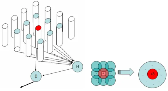
From researches of Anatomy and Physiology we find that V1 cells constitute a regular arrangement on cortex. Fig.2-5 is a schematic diagram showing stretch of cortex, and we may separate it into grids. Each grid has the same structure, which is called functional modules, and thus every point in retina corresponds to some functional modules.

As it can be seen in Fig. 2-4, every functional module contains different V1 cells which are selective to various orientation and frequency. It means that every point in vision has a complete set of linear filters with different property to analyze it, and this mechanism is the foundation of detecting 2nd-order boundary. The receptive field of V1can be modeled by a mathematic function which is called Gabor function,and We will discuss in detail in chap 3

.

(22)

Fig. 2-5 schematic diagram of cortex functional module

2.1.2 Linear filter theory

Linear filter theory about texture perception has been widely used in recent decades. It is based on the concepts of cortex functional module and linear system theory. There have been various linear models proposed by different laboratories, and the way they coming feature are different. In this thesis we adopt the one of them which is proposed by Chen, I [23].In this section we first introduce Linear system theory, and the detailed model used in this thesis is describe in Chap. 3.

(23)

Linear system

The world of input/output systems can be divided up into linear and non-linear systems. Linear systems are nice because the mathematics that describes them is not only well-known, but also has a mature elegance. On the other hand, it is a fair statement to say that most real-world systems are not linear, and thus hard to analyze...but fascinating if for that reason alone. That nature is usually non-linear doesn't mean one shouldn't familiarize oneself with the basics of linear system theory. Many times a non-linear system has a sufficiently smooth mapping that it can be approximated by a linear one over

restricted ranges of parameter values. The assumption of linearity is an excellent starting point--but must be tested.

The notion of a "linear system" is a generalization of the input/output properties of a straight line passing through zero. The matrix equation W⋅x= y is a linear

system. This means that if W is a matrix, x1 and x2 are vectors, and a and b are

scalars:

(

ax1 bx2

)

aW x1 bW x2 W⋅ + = ⋅ + ⋅

2.2 Preattentive Processing & Feature Integration Theory

（FIT, Triesman）

For many years vision researchers have been investigating how the human visual system analyses images. An important initial result was the discovery of a limited set of visual properties that are detected very rapidly and accurately by the low-level visual system. These properties were initially called preattentive, since their detection

seemed to precede focused attention. We now know that attention plays a critical role in what we see, even at this early stage of vision. The term preattentive continues to be used, however, since it conveys an intuitive notion of the speed and ease with which these properties are identified.

In this thesis we focus on preattentive boundary detection, and it means that we don’t use clustering or classification algorithm which resemble top-dowm process.

Feature integration theory of attention (FIT; Treisman & Gelade, 1980) proposes that there are two different stages of processing. In the first stage, basic

(24)

features of objects are analyzed in parallel and coded in specialized feature maps. In the second stage, focal attention is serially deployed to particular locations and serves to "glue" features in order to combine them into object representations. It was suggested that "without focal attention, features cannot be related to each other".

Fig. 2-6 a schematic diagram of FIT

A large body of evidence supporting FIT was obtained from visual search, texture segregation, or illusory conjunction experiments (Treisman, 1988, 1993;

Treisman & Sato, 1990). FIT’s features were determined in two ways: (1) by

determining pop-out boundaries between areas made up of different elements, and (2) by a visual search procedure (Julesz, 1981; Trisman, 1987).

Typically, in these types of experiments, multiple items are displayed and their numbers are varied to manipulate attentional load. In visual search experiments, targets are defined by a single feature or conjunctions of features. Participants are required to detect a target (or target area) among nontargets.

Fig. 2-7 illustrate an example that the effect of primitive. In Fig. 2-7 we want to find a target which is different to any other elements in (a) and (b) respectively, and it can be notice easily that this job is done more easily in (b). The reason in this example is that the “green x” in (b) possesses different color to other elements and color is a type of “primitive”, so se can feel the “pop-out” effect when we search the target. On the other hand, in (a) the “blue O” has the same color to “X” and the same shape to “red O”. There is not any unique “primitive” belonging to “blue O”, so we have to use our “attention” to search the target. This is a top down process and doesn’t belong to the definition of preattentive stage.

(25)

Fig. 2-7 an example to illustrate the effect of pop-out (a)no pup-out effect; (b) pop-out effect exists

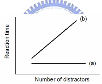
When Treisman did experiments similar to these demonstrations, she found that for targets that pop out (like in Fig. 2-7 (b)), the reaction time was fast no matter how many distractors were present in the display. This result is plotted as line (a) in Fig. 2-8. However, for targets that did not pop out (like Fig. 2-7 (a)), increasing the number of distractors increased the reaction time. This result is plotted as line (b) in Fig. 2-8.

Fig. 2-8 Typical results of a visual search experiment: (a) the result when pop-out occurs; (b) the result when there is no pop-out.

The primitive we used as 2nd-order feature is orientation, and Fig. 2-9 shows the pop-out effect by orientation. In Fig. 2-9 (a) the boundaries occur because the components have different orientations. In Fig. 2-9 (b) on the other hand, the central region indeed consists of elements different from elements in the rest region, but no pop-out boundary occurs. This is because the different elements in Fig. 2-9 (b) has same orientations components, and there is no other different “primitive” between the two elements in Fig.2-9 (b).

(26)

(a) (b)

Fig. 2-9 (a) element with different orientations; (b) elements with the same orientations(adapted from sensation and perception p.164)

(27)

Chapter 3 Hybrid-Order Texture

Boundary Detection

The physiological and psychophysical findings in the preceding section do not lead to a convenient computational model for the hypothesized cortical channels. In this chapter, a new boundary detection algorithm is proposed. This algorithm combines the 1st-order and 2nd-order features to model preattentive stage of human visual system. A simple hybrid-order channel model is described in the following.

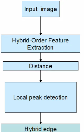
Fig. 3-1 shows a simplified flow-chart of the proposed algorithm. We first extract 1st-order by Gaussian low-pass filter and 2nd-order features by Gabor filters respectively. After feature extraction, every pixel of the output is an N+1 dimensional vector for (N Gabor filters and 1 Gaussian filter), and then we measure the difference of each pixel with its neighbor. Because pixels belong to the same region have similar feature, the difference between them should be small. Then we keep the value which is bigger than a threshold and make pixels of which value are smaller than threshold to zero. We would get coarse boundaries which have Gaussian-like distributions.

With boundaries which have Gaussian-like distribution, we may go a step further to thin these boundaries by local peak detection, and after this stage we will get boundaries similar to human visual system.

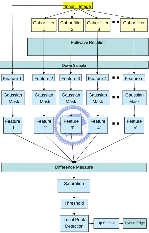
The proposed hybrid-boundary detection algorithm will be presented in detail, and the simplified block diagram is shown in Figure 3-1, and Fig. 3-2 is a detailed version of Fig.3.1. In Section 3.1, we first introduce hybrid-order Feature extraction step by step, and we will show how to measure the difference of pixels in feature space. In section 3.2, we illustrate the method that we use to thin the coarse boundaries which we have detected, and there we consider the saturation effect to enhance the results. In section 3.3, we introduce the way we utilized down sampling to accelerate the process.

(28)

(29)

Fig. 3-2 detailed block diagram for hybrid-order boundary detection algorithm FullwaveRectifior Down Sample Gabor filter 3 Feature 4 Feature 4’ Gaussian Mask Difference Measure Threshold Input Image Saturation Hybrid Edge Feature 1 Feature 1’ Gaussian Mask Gabor filter 2 Feature 3 Feature 3’ Gaussian Mask Gabor filter 1 Feature 2 Feature 2’ Gaussian Mask Gabor filter n Feature n Feature n’ Gaussian Mask Local Peak Detection Up Sample

(30)

3.1 Hybrid-Order Feature Extraction

In this section we introduce the way we extract first and second order features. 1st-order characteristics are processed by a collection of spatiotemporal filters, while the 2nd-order features are processed in a separate mechanism consisting of two filtering stages separated by a non-linearity. This second mechanism is more commonly known as the filter- rectify-filter cascade.

3.1.1 1st-order Feature Extraction

As we have seen in 2.1.1.1, the ganglion is accomplished by the so-called “center-surround” organization of the receptive field, in which its excitatory and inhibitory subfields are organized into circularly symmetric regions. The DoG model simply uses the difference of two 2D Gaussians to model the shape of receptive field here.

DoG function can be used in detecting boundaries. Two Gaussian filters with different values of σ are applied in parallel to the image. Then the difference of the two smoothed instances is computed. It can be shown that the DoG operator approximates the LoG (Laplacian of Gaussian) one which has been widely used in boundary detection.

We can think of the receptive field shape of a retinal ganglion cell as the linear spatial weighting function of the cell. That is, we can model the retinal ganglion cell as a linear neuron, where the receptive field tells us what the weights are. Using the function R(x,y) to characterize the receptive field shape using the DoG model, we compute the output of a model retinal ganglion cell as

=

∑

y x y x I y x R O , ) , ( ) , ( (3-1)

where I(x,y)is the input image.

For a whole array of retinal ganglion cells with identical receptive fields, we compute the output of each cell in the array as

∑

− − = y x y x I y y x x R y x O , 0 0 0 0, ) ( , ) ( , ) ( (3-2)

Here )O(x0,y0 is the output of the retinal ganglion cell whose receptive field is

(31)

The operation of Dog function can be divided into two stages, Gaussian convolution and gradient. Gaussian convolution is somehow like extracting the mean of local region which is we called 1st-order feature here, and gradient is measure the variation of 1st-order feature.

In order to combine 1st-order feature and 2nd-order feature, we only take Gaussian convolution to extract 1st-order feature here, and the gradient process will be done after combining 2nd-order feature.

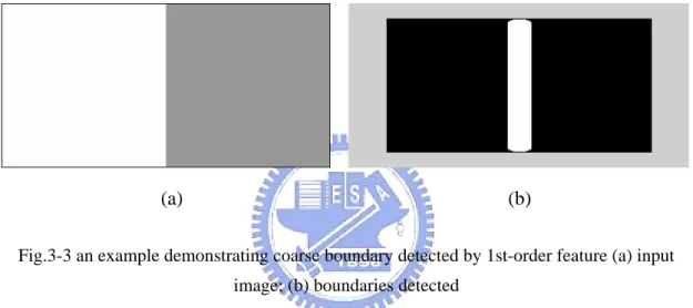
Fig. 3-3 illustrate the coarse boundary between two patterns with pure 1st-order features, and it is detected by only using first order feature.

(a) (b)

Fig.3-3 an example demonstrating coarse boundary detected by 1st-order feature (a) input image; (b) boundaries detected

In general, there should be more than one types of feature are mixed, and considering only first or second order feature is insufficient. Fig. 3-4 demonstrates the situation that patterns (D101-D102form brodatz texture) with hybrid-order feature but first order-feature is dominant.

In fact, test patterns in Fig. 3-4(a) are complement which means that 2nd-order feature are the same but pixels with high intensity and low intensity are exchange. In the left pattern background is white and thus its mean is bigger than the right one of which background is black oppositely. Fig.3-4(b) is the boundary we detect with 2nd-order feature only, and we can observe that the result is meaningless. Fig. 3-4(c) shows the result considering 1st-order feature, and it detects boundary successfully.

(32)

(a)

(b)

(c)

Fig. 3-4 An example demonstrating the effect of 1st-order feature in boundary detection: (a) 150×300 image (D101-D102); (b)boundary detected by 2nd-order feature; (c)boundary

detected by 1st-order feature

3.1.2 2nd-order Feature Extraction

3.1.2.1 Gabor Function

As we have mentioned in chap 2, the RF of V1 cells is orientation selective, and it can be modeled by function which was proposed by Gabor [24]. Gabor function consists of a Gaussian function modulated by a sinusoidal function, and it can be described as following:

(

)

[

jUx Vy

]

y x g y x h( , )= ( ', ')⋅exp2π + (3-3)

(

x',y'

) (

= xcosθ + ysinθ,−xsinθ + ycosθ

)

( )

⎪⎭ ⎪ ⎬ ⎫ ⎪⎩ ⎪ ⎨ ⎧ ⎥ ⎥ ⎦ ⎤ ⎢ ⎢ ⎣ ⎡ ⎟ ⎟ ⎠ ⎞ ⎜ ⎜ ⎝ ⎛ + ⎟⎟ ⎠ ⎞ ⎜⎜ ⎝ ⎛ − ⋅ ⎟ ⎟ ⎠ ⎞ ⎜ ⎜ ⎝ ⎛ = 2 2 2 1 exp 2 1 , y x y x y x y x g σ σ σ πσ (3-4) here,

( )

x y h , : Gabor function

( )

x y g , : Gaussian function

(33)

(

x',y'

) (

= xcosθ + ysinθ,−xwinθ +ycosθ

)

: Rotated spatial-domain rectilinear coordinates x σ : STD of Gaussian in x axis y σ : STD of Gaussian in y axis

The shape of two-dimensional Gaussian function is controlled by aspect ratio

(

σx/σy

)

andσx,σy which are standard deviation of Gaussian function in

x-axis and y-axis in spatial domain respectively. In most cases, letting σx =σy =σ

is a reasonable design choice. The complex exponential component works on the center frequency

( )

F and orientation

( )

φ of the Gabor filter. In other word, the complex exponential component decides the place where frequency response of Gabor filer lies. F is given by

(

₂ ₂

)

1/2

V U

F = + ,φ ≡tan−1

(

V/U

)

and U is spatial frequency in x axis, and V is spatial frequency in y axis.

A Fourier transform of (3-3) is given by

[

]

(

)

(

[

]

)

[

]

⎭ ⎬ ⎫ ⎩ ⎨ ⎧₋ ₋ ₊ ₋ = 2 2 ' ' 2 1 exp ) , (u v u U v V H σ_x σ_y (3-5)

(

) (

)

[

u−U ', v−V '

]

=

[

(

u−Ucosθ +

(

v−Vsinθ

)

) (

,

(

− u−U

)

sinθ +

(

v−V

)

sinθ

)

]

(3-6) shows that Gabor filter in frequency domain is an adaptive band-pass filter and has the shape of Gaussian. Because ofσx =σy =σ , the parameter θ is not needed and

(3-3) simplifies to

(

)

_[

₍

₎

_]

Vy Ux j y x y x h + ⎭ ⎬ ⎫ ⎩ ⎨ ⎧₋ + = π σ πσ exp 2 exp2 2 1 ) , ( ₂ 2 2 2

In practice the Gabor function can be divided into real (even) part and imaginary (odd) part as

( ) ( )

x,y g x,y cos(2 Fx') h_c = π (3-6 )

( )

x,y g

( )

x,y sin(2 Fx') h_s = π (3-7) φ φ sin cos ' x y x = +

It can be seen that (3-6) and (3-7) are very similar, and (3-7) is just a phase shift version of (3-6). Both of them can extract local feature of spatial domain, and based on psychophysical grounds, Malik and Perona provided some justification fro using

(34)

even-symmetric filters only. In this thesis we use real-valued, even-symmetric Gabor filters.

Gabor function constructs a complete but nonorthogonal basis set. An example has presented in 0, where Fig. 3(a) is a standard Gabor type filter in the time domain, and Fig. 3(b) is in frequency domain. Expanding the signal using this basis provides a localized frequency description.

(a) (b)

Fig. 3-5 An example of 2D Gabor type filtering. (a) is a standard 2D Gabor type filter in time domain, and (b) is in frequency domain.

An important property of Gabor filters is that they have optimal joint localization, or resolution, in both the spatial and the spatial-frequency domains. By signal processing we know that a Fourier transform of Gaussian function is still Gaussian function, and by “uncertainty principle” we know that Gaussian function is the only function that can reach the optimal constraint of uncertainty principle. Uncertainty principle describes the optimal resolution in both the spatial and the spatial-frequency domains. (Uncertainty relation for resolution in space, spatial frequency, and orientation optimized by two-dimensional

Visual cortical filters)

When we observe signal in both spatial and the spatial-frequency domain, Heisenberg Uncertainty Principle state that decreasing the deviation in frequency (increasing the resolution) must result in an increase in the deviation in time (decrease in resolution) and vice versa.

Gabor has first recognized and introduced a time-frequency version of Heisenberg’s inequality:

(35)

π

σ

4

1 ≥

f t

Where σt and σf are the time and frequency standard deviations respectively.

Gabor filter is just modulation of Gaussian function. Gabor has been proved that this action only cause movement in frequency domain, and it wouldn’t affect the resolution of Gaussian function in spatial and the spatial-frequency domain. It means that Gabor function inherit property of Gaussian possessing optimal resolution in both domain, and this property is why Gabor filter is suitable for texture segregation.

3.1.2.2 Full-Wave Rectification

Like other filter- rectify-filter model, rectifying operation is taken after convolution by Gabor filters. It has been generally acknowledged that V1 cells have a property like half wave rectification property, and the intervening rectification ensures that the fine-grain positive and negative portions of the carrier do not cancel one another when smoothed by the later filter. The Rectifying operation also break the identically equality between linear filter theory and Fourier transformation

.

Fig. 3-6(b) demonstrates the output after Gabor filtering without rectifying, and Fig. 3-6(c) is after rectification. White pixels in the image reflect the pixel that Gabor has detected the matching feature, and it is similar that our V1 cells have response. Because the restriction of display, there are some pixels with negative response in Fig. 3-6(b) doesn’t appear. In Fig. 3-6(c) it can notice that there are two regions are separated more apparently, and this is because of the rectification turning the negative response to positive.

(36)

(a)

(b)

(c)

Fig. 3-6 an example demonstrates the effect of rectifying (a) input; (b) output without rectifying; (c) output with rectifying

(37)

3.1.2.3 Gaussian post filter and difference measure

Gaussian post filter

After being stimulated by bars with specific orientations, the output of V1 cells responding to similar orientation will aggregate together. The region with the same property will respond stronger than regions which consist of elements with different properties, and it is consistent with the “localization” property of texture. We can simulate this effect by a Gaussian post filters, it is somewhat like averaging with different weighting which is inverse proportion to distance to the center of the post filter. In the field of texture segmentation, Gaussian smoothing is an important procedure to eliminate features that varying abruptly.

Fig. 3-7(b) shows the result after rectifying without Gaussian filter, and Fig. 3-7(c) is the result that 3-7(b) after Gaussian filter. In 3-7(c) there is a ramp-like feature profile, and the next step is to detect the position where the variation of difference is maximum.

(a)

(b)

(c)

(38)

Difference measure

After extracting features of each local region, the features can be described by an N-dimensional vector, and each feature vector can be regard as a point in N-dimensional space. Similar to [23], the difference is represented by the distance in N-dimensional space.

Fig. 3-8 illustrates the schematic diagram of the feature vector in 3-dimensional space.

*

Fig. 3-8 an schematic diagram of an 3-dimensional feature space

T

here is an important property in texture that pixels aggregate together usually have similar feature, so the position information is also an important feature. Because the reason we above, gradient is a common operation used in some algorithms [12]

.

In this thesis, we only compute the difference between features of each pixel to pixels right behind and below to it.

(39)

3.1.2.4 Gabor filter bank

Besides orientation selectivity, Gabor filters also have frequency selectivity with different parameter. With these two properties, Daugman extended the original Gabor filter to a two-dimensional (2D) representation [26]. There have been many researches about Gabor filter bank. Jain and Farrokhnia [11] suggested a bank of Gabor filters, i.e., Gaussian shaped band-pass filters, with dyadic coverage of the radial spatial frequency range and multiple orientations.

Because our goal is design an algorithm which can be implemented by CNN, the structure can’t be too complex. In this thesis we use totally sixteen Gabor filters to extract 2nd-order feature to do our experiments. All these Gabor filters have the same Gaussian shape in frequency and scatter uniformly in four orientations and four frequency bands. Fig (a) illustrates frequency response of Gabor filter with different orientation in the same frequency band, and Fig (b) illustrates Gabor filters with different frequency band in the same orientation. Fig. 3-8(a) demonstrates the frequency response of the Gabor filters with orientation in0°,45°,90°, 135°

respectively. Fig. 3-8(b) demonstrates the frequency response of the Gabor filters with center frequency in 0.03125, 0.0625, 0.09375, 0.125 cycles/pixel respectively.

(40)

(a)

(b)

Fig. 3-9 frequency response of (a) Gabor filters in different orientation (b) Gabor filters in different frequency band

(41)

3.2 Saturation & Local maximum Detection

3.2.1 Saturation

In our algorithm, there is a problem when the number of test patterns increases. When the number of tests patterns in an image is greater than two, there would be more than one boundary existing. Because these boundaries usually do not have similar intensity, choosing threshold becomes an important problem.

In this thesis we choose the mean of difference of total pixels as threshold, and the situation occur most frequently is that some boundaries with relative lower magnitude is eliminated. This is because of a relative huge region being considered to measure local feature, and the scale of difference between different patterns vary enormously. Obvious boundaries and cause relatively great difference and raise the mean of difference, and the boundaries which are not so obvious causing relative low difference will be eliminate.

We use natural log transformation to simulate the saturation effect to alleviate this problem. It can suppress strong responses which may affect the mean (threshold) to much, but still keep the position of maximum difference where we assume boundaries lying.

Strength of responses reflects the level differences between two local regions, but it may be not so linearly consistent to our perceptional feeling. In biology, and the response should not linear proportional to stimulations.

In human vision system the dynamic range of response are limited, and the range of response will not linearly proportional to stimulate. Natural log transformation is an ordinary and important operation. Natural log transformation stretch the range of lower responses where we need to judge whether there are boundaries or not. It is good when we take threshold and quantization. In chap. 4.2.3 there will be experimental results demonstrating the effect of natural log transformation.

3.2.2 Local Maximum Detection

The coarse boundaries detected after taking threshold are too thick, and local maximum detection is used to thin it. It is assumed that the difference between

(42)

different patterns should be maximal at their boundary, and the boundary will be right there. The object here is to detect a local maximum of difference we remain at this stage.

Algorithm of local peak detection:

1) Here we scan row by row and column by column to find local maximums in x and y axes.

2) Sort the peaks we find in 1) in descending order.

3) Keep points with higher order in each line and column, and the output is binary. The values at that pixel regarded as boundaries (points with higher order) are 255, and others are 0.

The number of peak-points we keep in 3) is depending on the complexity of input image, and in our testing images we use two.

Fig. 3-10 is an example demonstrates the peak detection in the algorithm. Fig. 3-10(a) is an input image, and (b) is the detected coarse boundary. Fig. 3-10(c) is the 3D version of 3-10 (b), and in this figure the vertical axis is intensity. 3-10(d) is the result of 3-10 (c) by taking peak detection. 3-10(e) is the superposition of 3-10(a) and 3-10(c). From 3-10(e) we can observe that the detected boundaries have high accuracy which is consistent to our assumption.

(43)

(a)

(b)

(c)

(d) (e)

Fig. 3-10 (a)input (b)coarse boundary (c)3D version of (b) (d)(c)after peak detection (d)superposition of (a) and (d)

(44)

3.3 Down sampling and up sampling

After rectifying 2nd –order features of different orientations have been extracted (as we have mentioned in 3.1.2.2), and the output of each channel has the same size to input images (in our experiments each texture pattern has 640×640 pixels). The amount of features is proportional to the number of channels. With the number of channels increasing, it cause heavy computational loading in following processing, and we improve this problem by down sampling feature space (in our experiments we down sample by 3).

By choosing appropriate down sampling rates we can accelerate the following processes without losing too much accuracy. After boundaries have been detected, we will up sample before output. It will map detected boundaries to the corresponding position in original input.

This mechanism is similar to human vision, and trade-off of spatial accuracy and computational loading is a common problem in human vision system and the proposed algorithm. In fact the whole visual pathway is like serial processes of information extraction and data compression.

Without attention, human vision generally has low resolution in the field of vision, and even with attention we only have high resolution in a relatively tiny proportion of the field of vision. Although in this thesis we only consider the Preattentive situation, we still have acceptable spatial-accuracy for boundary detection which can be observed after local peak detection.

(45)

Chapter

4 Experimental Results and

Discussion

In this chapter we will apply our algorithm to images which consist of a number

of different test pattern. Most of them are synthesized by textures from “Brodatz

texture database” which is derived from the Brodatz album, and it also has become a

standard for evaluating texture algorithms. It has a relatively large number of classes

(112 classes), and a small number of examples for each class. Each texture pattern we

used here are 640*640 pixel 8-bit gray-scale images respectively. When computing

the texture features for pixels near the image boundary, we assume that the image is

extended by its mirror image—often referred to as the even reflection boundary

condition. In section 4-1, we first introduce parameter selection. In section 4-6, there

are some important properties are introduced. In section 4-3, we will have a widely

test on synthesizing different textures by the proposed algorithm. In section 4-4, the

(46)

4.1 Parameters Selection

There are some parameters need to be selected:

1. The number of Gabor filters and

(

U,V,σ

)

of them which decide the shape and orientation of Gabor filters in frequency domain.

Gabor filtering is computation intensive, and increasing the number of Gabor filters will increase computation loading dramatically. On the other hand, unnecessary and useless feature extracted by wrong-designed Gabor filters may cause wrong boundaries.

2. σ_g of the post Gaussian filter, which decides the smoothing level.

Increasing σ can eliminate more noise, but the accuracy of the boundary may decrease. Because both Gabor filters and Gaussian filters have spatial information, the values of σ_g must cooperate with σ to obtain a better result.

Designing parameter above is an important but sophisticated problem. Designing center frequencies of Gabor filters is most discussed in filter-design approaches. They are including the unsupervised methods such as algorithm proposed by Jain and supervised methods such as algorithm proposed by Dunn [27]. Algorithm in this thesis belongs to unsupervised method which means that all information of input pattern is unknown. Nevertheless, the emphasis of this paper is not on optimizing the design of Gabor filter, but rather proposing a simple algorithm modeling early vision and being able to be implemented on CNN. Parameters in Table 4.1 are empirically chosen and they are all the same in the following experiments without indicating specifically

Parameters Value

Pattern size(Brodatz texture) 640*640

pixels

Orientation

φ 0°

,

45°

,

90°

,

135°

Center frequency

F

1/32, 1/16, 3/32, 1/8 cycles/pixel

σ

of Gabor filter

16

pixels

Down sampling rate M

3

g

(47)

Mask sizes of Gabor and Gaussian

3

σ

, 3

σg

Table 4.1 parameters of experiments in Chap. 4

4.2 Experiments of Hybrid-Order Boundary

Detection

4.2.1 Experiment 1: effects of multi-band Gabor filters

In this experiment we will demonstrate the reason why we need multi-band

Gabor filters. During this experiment we close the channel of 1st-order which means that we only consider 2nd-order features when detecting boundaries. From Fig. 4-1-1 to Fig. 4-4 we will demonstrate 2nd –order feature image in the direction of 0°, 45°,

°

90 , 135°_{in each single band. The center frequencies of four bonds are 0.03125,}

0.0625, 0.09375, 0.125 cycles/pixel.

(48)

Band 1(

F =0.03125

cycles/pixel)

(a) (b)

(c) (d)

(49)

Fig. 4-1 feature image of band 1(a)0° (b)45° (c)90° (d) 135° (e) coarse boundaries (d) (e) after peak detection

Band 2(

F =0.0625

cycles/pixel)

(a) (b)

(c) (d)

(50)

Fig. 4-2 feature image of band 2 (a)0° (b)45° (c)90°_(d)135°_{(e) coarse boundaries (d) (e)}

after peak detection

Band 3(

F =0.09375

cycles/pixel)

(a) (b)

(c) (d)

(51)

Fig. 4-3 feature image of band 3 (a)0° (b)45° (c)90° (d) 135° (e) coarse boundaries (d) (e) after peak detection

Band 4(

F =0.125

cycles/pixel)

(a) (b)

(c) (d)

(52)

Fig. 4-4 feature image of band 4 (a)0° (b)45° (c)90° (d) 135° (e) coarse boundaries (d) (e) after peak detection

4 Bands simultaneously

(c) (d)

(e)

Fig. 4-5 (c) coarse boundaries (d) (c) after boundary detection (e) superposition of (d) and input

From Fig. 4-1 to 4-4 we can find that there are always some boundaries remain undetected, and we can’t find all boundaries by a single band in this example. Fig. 4-5 shows the result of boundary detection by four bands simultaneously, and it can be found that all boundaries are detected.

(53)

4.2.2 Effects of hybrid-order features

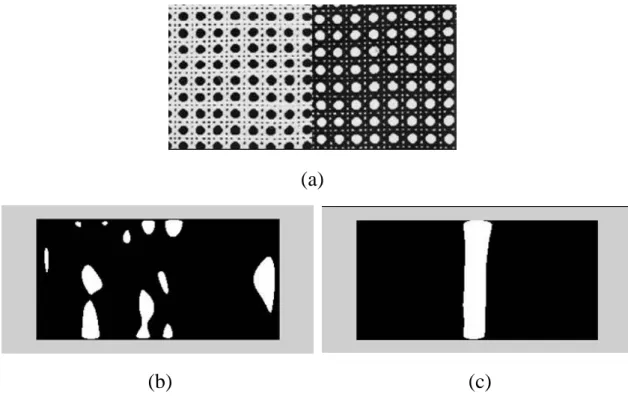
In this experiment we will demonstrate the reason why we should consider 1st –order and 2nd-order features simultaneously. Fig. 4-6(a), (b), (c), (d) demonstrate the coarse boundaries and boundaries after peak detection by 1st –order and 2nd –order features respectively. In Fig. 4-6(a), (b) it only detects the boundaries in lower part which is obvious different in 1st -order features, and in Fig. 4-6(c), (d) it only detects 2nd –order boundaries. In these four images it is found that it is insufficient to detect all boundaries by a single order feature. In fig. 4-6(e), (f) hybrid-order features are considered simultaneous and all boundaries are detected.

(54)

(a) (b)

(c) (d)

(55)

(g)

Fig. 4-6 (a)coarse boundaries detected by 1st-order features (b)(a)after detection (c)coarse boundaries detected by 2nd-order features (d)(c)after detection (e)coarse boundaries detected by

hybrid-order features (f) (f)after detection (g)superposition of (f) and input

There is still one thing that we can observe in this experiment. As fig. 4-6 shows, the boundaries detected by 1st –order features are thinner than those detected by 2nd –order. The reason of this property is that 2nd –order feature is extracted by Gabor filter before Gaussian convolution, and this process would blur the boundaries we detected at last. The second order feature processed by Gabor and Gaussian filters can be regarded as being blurred twice, so 2nd –order boundaries would be thicker. This property will also appear in Chap. 4.3 where we will demonstrate more experimental results.

4.2.3 Saturation effects

Fig. 4-7 is am example illustrate the effect of saturation. Fig. 4-7 (a) is the coarse boundary detected after Gaussian filter before thresholding without taking natural log transformation, and 4-7 (b) is 4-7 (a) after natural log transformation. Fig. 4-7 (c), (d)

(56)

are (a), (b) after thresholding respectively. Comparing Fig. 4-7 (a) and (b), we can notice that contrasts of strong difference (response) in (a) are compressed and contrasts of weak difference are raised after natural log transform. In Fig. 4-7 (b) there are strong and weak interdistances between different textures and intratdistances reflecting the nonuniform property of the right-up texture (Brodatz texture: D62). These strong responses may raise the threshold (mean of responses) and eliminate weak ones which we should keep.

Fig. 4-7 (e) is the 2D version of Fig. 4-7 (c) and from both of them we can find that weak boundary between D6 and D109 are eliminated. On the other hand, all boundaries are kept in Fig. 4-7 (f).Fig.4-7 (g) and (h) shows the result of Fig.3-9(f) after local maximum detection, and the output is approximately consistent to our visual perception.

(57)

(a) (b)

(c) (d)

p

(58)

(g) (h)

Fig. 4-7 (a) coarse boundaries without log transform; (b)(a) after log transform; (c)(a)after thresholding; (d)(b) after thresholding; (e)2D version of (c); (f) 2D version of (d); (g)(f) after

peak detection; (h)superposition of input and (h)

4.3 Collection of Testing Results by Hybrid-Order

Boundary Detection

In this section the proposed algorithm is tested by a variety of textures randomly chosen from “Brodatz texture database”. For saving the space, we synthesize five textures in each image. There would be eight boundaries between two attached textures. We will show coarse boundaries, boundaries after peak detection, and superposition of boundaries and tested image in order. There are totally 57 testing results in the follow, and all parameters we use here are the same as we have mentioned in section 4.1.

In this section we classify the results of our experimental results into three categories roughly. In section 4.3.1 we collect the results which all boundaries are detected. In section 4.3.2 we collect the results which there are some boundaries missing. In section 4.3.3 we collect the results which have the poorest results.

4.3.1 Results which all Boundaries are Detected

(59)

or similar texture elements. Natural textures usually have some nonuniform part, but textures we use in this section are uniform in most part. In this section, all boundaries between different textures are detected and small edges within single texture are also detected. These results are consistent to our visual perception.

(60)

(61)

(62)

4.3.2 Results which some Boundaries are not Detected

In this section we demonstrate results that some boundaries aren’t detected. Some of textures in this section are not so uniform such that boundaries within single

(63)

texture are more obvious than boundaries between different textures. In some cases, two textures have similar features, and the boundaries can’t be detected as we can’t distinguish them at our first sight.

(64)

(65)

(66)

(67)

(68)

(69)

(70)

(71)

(72)

4.3.3 Worst Results

In this section we synthesize all textures which are not in our definition of uniform texture, and the results are poorest among all test images. Although it can’t detect boundaries as testing images in 4.3.1 and 4.3.2, the results still can reflect some meaningful boundaries. In fact there are not obvious boundaries between two different textures if we see by our eyes. From the image of coarse boundaries and input we can find that this algorithm detected the most obvious edges in these nonuniform textures, and this result is still consistent to our perceptional experience.

(73)

4.4 Discussion of Accuracy

In this section the accuracy of the proposed method is discussed. The way we estimate the error is as fellow:

1. Only the case that synthesizes two texture patterns in Brodatz texture is considered. In the algorithm every boundaries are proposed independently. It is also hard to judge accuracy if considering multi-boundaries simultaneously when some boundaries are detected and some are not.

2. The distance between the answer and the result detected by the algorithm is measured in the condition of boundary being detectable. We define the error by dividing measured distance into the number of total pixels.

example:

(a) (b) (c)

早期視覺下之生物啟發式混合質感邊界偵測模型

國 立 交 通 大 學

電機與控制工程學系

碩 士 論 文