考量大眾運輸優先之可適性都市交通號誌控制系統

國

立

交

通

大

學

資訊科學與工程研究所

碩

士

論

文

考量大眾運輸優先

之可適性都市交通號誌控制系統

An Adaptive Urban Traffic Signal Control System

with Bus Priority

研 究 生：張慈麟

指導教授：簡榮宏 博士

考量大眾運輸優先之可適性都市交通號誌控制系統

An Adaptive Urban Traffic Signal Control System

with Bus Priority

研 究 生：張慈麟

Student：Tzu-Lin Chang

指導教授：簡榮宏

Advisor：Rong-Hong Jan

國 立 交 通 大 學

資 訊 科 學 與 工 程 研 究 所

碩 士 論 文

A Thesis

Submitted to Institute of Computer Science and Engineering College of Computer Science

National Chiao Tung University in partial Fulfillment of the Requirements

for the Degree of Master

in

Computer Science July 2012

Hsinchu, Taiwan, Republic of China 中 華 民 國 101 年 7 月

i

考量大眾運輸優先之可適性都市交通號誌控制系統

研究生：張慈麟

指導教授：簡榮宏 博士

國立交通大學資訊科學與工程研究所

摘

要

近年來，隨著經濟快速成長以及都市高度開發，交通壅塞已經成為各都市的 主要問題，因此交通號誌控制一直是智慧型運輸系統(Intelligent Transportation System, ITS )中重要的一部分。巴士可搭載高乘客的特性使其成為非常適合都市 環境的交通工具，因此巴士優先權也成為交通號誌控制系統中重要的一部分。巴 士具有不同於一般車輛的特性:較多的乘客數量、巴士預計到站時間以及前後班 次間隔等。先前有關巴士優先權的研究著重於減少平均等待時間，但他們並沒有 同時考量到以上所提的種種巴士特性以及會對一般車輛所造成的影響。在此篇論 文中，我們提出一可適性即時交通號誌控系統，藉由路邊的感測節點以及巴士上 之車載機等方式收集即時交通資訊，計算出各時相所需的時間以及其所擁有的效 益值和公車優先權，並依此控制交通號誌藉以減少乘客等待時間以及有效調整巴 士的航班。實驗結果顯示我們的方法可以有效減少乘客等待時間以及有效改善巴 士到站時間誤差以及前後班次間隔誤差。

ii

An Adaptive Urban Traffic Signal

Control System with Bus Priority

Student：Tzu-Lin Chang Advisor：Dr. Rong-Hong Jan

INSTITUTE OF COMPUTER SCIENCE AND ENGINEERING

NATIONAL CHIAO TUNG UNIVERSITY

Abstract

In recent years, with the economic development and urbanization, traffic congestion

has become a serious problem in urban environments. So, traffic signal control plays a

key role in Intelligent Transportation System (ITS). Particularly, bus system can carry

a higher capacity of passengers, which help to relief traffic jam in cities. Thus, it is

important to consider bus priority during traffic light control. However, different from

ordinary vehicles, bus system has some unique features, including higher capacity of

passengers, fixed routes and specific requirements on bus schedules and headways. In

this thesis, we propose an adaptive traffic signal control system with bus priority. By

collecting traffic information from roadside detectors and buses, we jointly consider

how the above factors change buses priority and the impact to ordinary vehicles.

Simulation results show that our system can significantly reduce total waiting time of

iii

致謝

首先學生要感謝指導多年的指導教授簡榮宏博士，從大學專題研究起，老師 對學生的諄諄教誨，使學生在課業、學術研究上和待人處事方面皆獲益良多，在 此獻上學生最高的謝意。同時，也感謝陳健教授以及易志偉教授花費大量時間對 學生論文提供意見以及指教，使本論文更臻完善，在此深表感激。 計算機網路實驗室的所有成員於我研究生活所提供的幫助，使我在兩年的研 究生涯感到無比充實。感謝學長們(安凱、家瑋)於我論文研究的大力幫助，以及 精闢的建議，在此致上深深的謝意。也感謝同學(唯義、紹閔、曰慈)以及學弟們 (和家、秉琨、瑋劭、景祥)的共同努力，使我能順利完成學業研究以及豐富我的 研究生活。 最後我要感謝我的家人以及眾多在這段時間中支持我走過研究生活的朋友 們，感謝你們一路上的支持與鼓勵，讓我可以堅持到最後並完成人生重要的里程 碑。在此，本文獻要獻給一路關懷勉勵我的家人以及朋友們。

iv

Contents

Chapter 1 Introduction ... 1

Chapter 2 Related Work ... 4

2.1 Traffic Signal Control ... 4

2.2 Bus Priority ... 5

Chapter 3 Adaptive Traffic Signal Control System... 8

3.1 System Overview ... 8

3.2 System Flow ... 10

Chapter 4 System Design... 12

4.1 Phase Length Determination ... 12

4.2 Phase Demand Determination ... 14

4.2.1 Passengers’ Waiting Time ... 15

4.2.2 Bus Schedule Delay ... 17

4.2.3 Bus Headway Deviation ... 18

4.2.4 Phase Demand Function ... 20

Chapter 5 Simulation ... 22

5.1 Simulation Environment ... 23

5.2 Simulation Results ... 26

5.3 A Simulation in Real Urban Environment ... 33

v

List of Figures

Figure 1. A typical four-phase cycle at a four-direction intersection ... 5

Figure 2. System architecture ... 9

Figure 3. Intersection model ... 10

Figure 4. System flowchart ... 11

Figure 5. Distance between stop line and the farthest vehicle of phase1 ... 13

Figure 6. Example of calculating time to disperse vehicles. ... 14

Figure 7. The current location and predicted location of the vehicle ... 16

Figure 8. Passengers’ waiting time cumulated in a lane ... 16

Figure 9. The headway between two buses ... 19

Figure 10. An Example of random network and bus routes ... 24

Figure 11. Total waiting time of buses ... 26

Figure 12. Total waiting time of vehicles ... 28

Figure 13. Total waiting time of passengers ... 29

Figure 14. Bus schedule delay in a bus stop at a pivot intersection... 30

Figure 15. Bus headway deviation ratio in a bus stop at a pivot intersection ... 31

vi

List of Tables

Table 1. Simulation parameters ... 25

Table 2. Total waiting time of buses and average waiting time of each bus in one

intersection 27

Table 3. Total Waiting time of buses and average waiting time of each vehicle in one

intersection 28

Table 4. Total waiting time of passengers and Average waiting time of each vehicle in

one intersection ... 29

Table 5. Average schedule delay time and Variances of buses at a pivot intersection 30

Table 6. Average headway deviation ratio and variances of buses at a pivot

intersection 32

Table 7. Simulation result ... 32

1

Chapter 1

Introduction

Intelligent Transportation System (ITS) is a system that incorporates advanced

electronics technologies into transportation infrastructure and vehicles, in order to

improve driving safety, transportation time, fuel consumption and services.

Traffic signal control systems [1-2] plays a key role in ITS. It improves the

transportation efficiency by detecting real-time traffic information and choosing suitable

strategies to adapt to different traffic scenarios. With the increasing motorization,

urbanization, population growth and changes in population density, traffic congestion

which increases travel time, air pollution and fuel consumption has become an important

problem of the world today. An improper traffic signal control strategy may cause severe

traffic jam, particular at road intersections.

The development of intelligent design in traffic light control depends on sensing

techniques. In addition to traditional methods like inductive loop detectors and video

vehicle detector [3], there are many advanced sensing techniques have been proposed.

For instances, Wireless Sensor Networks (WSNs) [4] and Vehicular Ad hoc Networks

(VANETs) [5] have been adopted in ITS in recent years which extend the sensing

coverage and require less expensive cost. Furthermore, new techniques provide more

2

In recent decades, with the increasing attentions on environment protection, people

have begun be aware of the importance of reducing air pollution. More and more

passengers are willing to utilize public transport system instead of driving their own cars,

in order to protect the environment as well as to avoid traffic congestion. Bus system is a

major segment in public transport system of urban area. Bus system has several unique

features different with ordinary vehicles. First, buses have higher capacity to carry more

passengers (usually 20 to 35 persons) than ordinary vehicles (1 to 4 persons). It means

that more people can be benefited from a waiting time decrement if we gave each bus a

higher priority. Second, each bus has a fixed schedule which specifies the arriving time

of the bus at each bus stop. People can save time if the bus arrived at bus stops on time.

The third feature is that bus system has a specific requirement on the time interval

between any two successive buses, i.e., the headway, in the same bus route. Keeping a

regular headway would make the bus system more trustable and let people be more

willing to take buses.

A number of methods [18]-[22] have been proposed and adopted to benefit buses.

However, most of them focus only on reducing the bus waiting time and pay little

attention on the features of buses mentioned above. Besides, none of them consider the

impact to ordinary cars, because allocating more passing time to buses could also scarify

the passing time of other vehicles. Moreover, the previous works usually assume a fixed

phase sequence, which however, has little flexibility to deal with the sudden traffic

changing or an approaching bus.

In this thesis, we propose an adaptive traffic signal control system with bus priority,

abbreviated as ATCB. The system is based on a non-fixed phase scheme to deal with the

real-time traffic changing and approaching buses effectively. At each intersection, our

3

schedule delay and headway deviation of buses, to select the most suitable signal.

Simulation results show that ATCB can improve the waiting time of both buses and

ordinary vehicles, keep bus schedules on time and regular bus headways.

The rest of the thesis is organized as follows. In Chapter 2, we review the review

various traffic signal control strategies and related works with bus priority. Then, we

give an system overview and system flow in Chapter 3. The detailed descriptions of

ATCB are presented in Chapter 4. In Chapter 5, we evaluate the proposed system by

simulation and compare it with other methods. Finally, conclusion and future works are

4

Chapter 2

Related Work

In this chapter, we review the previous studies and related works .In section 2.1, we

introduce the existing traffic signal control systems. In section 2.2, we introduce some

articles about bus priority.

2.1 Traffic Signal Control

There are a lot of traffic signal control systems have been implement worldwide, such

as SCOOT [1] and SCATS [2]. These systems control the movement of vehicles by

allocating time to the split of each phase in a cycle. Phase means a combination of green

and red signals that vehicles in some specific directions can pass through the intersection

at. In general, because the right-turning movement doesn’t have conflict with other

movement, it is included in straight-going movement. Split refers to the length of a

phase in a cycle.

These traffic signal control method can be classify to two categories length of the

defined plan. The systems of the first one [1], [2], [6]-[8]which make little changes on a

predefined signal or choose a signal plan among a pre-specified set. The second category

[9]-[15] decides to switch or not the traffic lights at each step. The first one usually

focuses on long-term performance, but it can’t respond well to dynamic changing like

the second one.

5

is fixed [9] or non-fixed [10]. Obviously, the fixed phase sequence scheme is more

acceptable for drivers, because it is similar to the traditional methods we are familiar

with.

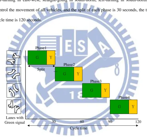
A typical four-phase cycle at a four-direction intersection is shown in Figure 1, there

are four phases: Phase1, Phase2, Phase3 and Phase4(straight-going in east-west,

left-turning in east-west, straight-going in south-north, left-turning in south-north) to

control the movement of all vehicles, and the split of each phase is 30 seconds, the total

cycle time is 120 seconds.

G Y G Y G Y G Y 120 90 60 30 Cycle time Split Phase1 Phase2 Phase3 Phase4 Lanes with Green signal

Figure 1. A typical four-phase cycle at a four-direction intersection

2.2 Bus Priority

In[18], it first summarizes how bus priority at traffic signals works within iBUS(an

6

the bus send its GPS location information to the signal, so that the signal can predict the

arriving time of the bus and decide whether to extend current phase for the bus. This

paper then explores the effects of GPS locational errors on bus priority benefits, and we

can know the impotence of accurately predicting.

In [19],this work also decides whether to extend the current phase after receiving the

request of the incoming bus. But it has considered the situation of buses to design a

headway-based strategy or a schedule-based strategy. So if two or more buses request

the signal different phases, the signal will meet the request with the highest priority (this

not considered in [18]).

Unlike [18] and [19], some works[20] adopts a fixed cycle-time plan, it allocates time

to split of each phase at the start of the cycle, and it will change its plan after receive

request of bus. This method can meet multiple requirements by modifying its original

plan, it can not only extend the phase, but also can make the required phase occur more

early. If there are two or more requests from different buses conflict, it uses a

headway-schedule bus priority to decide what changing should be taken.

In [21], it changes the signal not only based on information of buses but also

information of roads and ordinary vehicles. It considers several elements: First, the

remaining time until the traveling bus in the current green signal phase arrives at the

stop line. Second, the waiting time duration that buses in the next green signal phase

stay on red signal. Third, the ratio of the effective green signal time duration to the green

signal time duration, where effective green signal time duration means the duration

between vehicles arriving the stop line and pass through the stop line. Fourth, the

number of vehicles in the link between the intersection and the adjacent downstream

intersection, if the high number refers the downstream intersection will be possible to

7

extend the current phase.

Some researches focuses on reducing passengers’ waiting time for buses arriving at bus stops instead of passengers’ waiting time for signals on buses. [22] shows that greater regularity benefits could be achieved through a strategy where priority for a bus

is based not only on its own headway but also the headway of the bus behind.

However, these works about bus priority have some drawbacks. First, they mostly

focus on reducing bus waiting time and can’t concern about features of buses in the same time. Second, they may not consider the impact to ordinary vehicles by control

signals for buses. Third, these works usually control signal with a fixed phase sequence

which have little flexibility to change to the phase has highest priority due to the more

vehicles or delay buses.

8

Chapter 3

Adaptive Traffic Signal Control

System

In this chapter, we introduce out adaptive traffic signal control system .In section 3.1,

we propose our system architecture. In section 3.2 we introduce assumptions of the

system.

3.1 System Overview

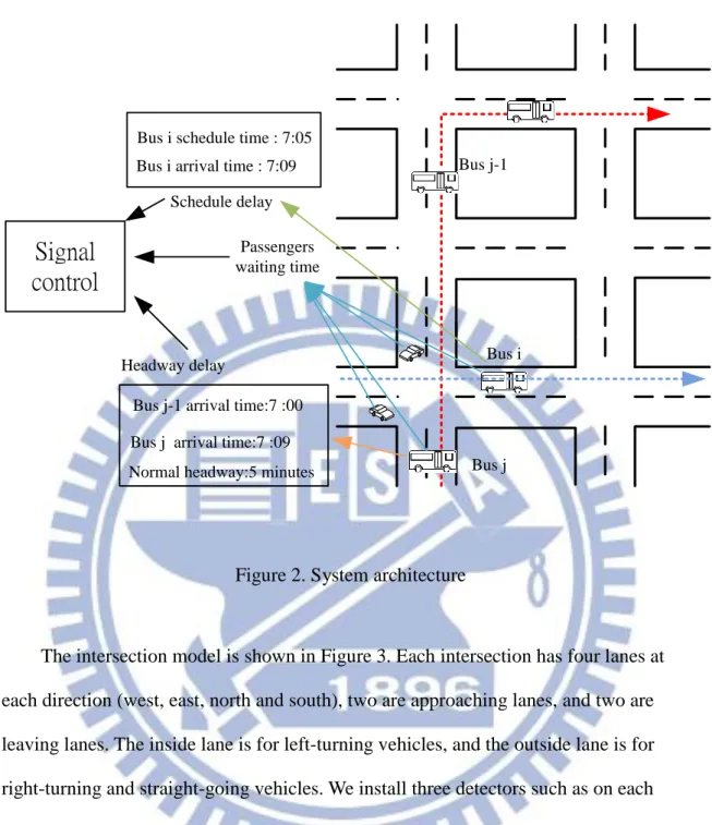
As shown in figure 2, intersections collect information includes the location and

speed of vehicles, headway deviation and schedule delay of buses at the intersection. In

order to deal with the real-time changing of traffic flow, we adopted a non-fixed phase

sequence [10] at each intersection. For each intersection, when the current phase is over,

we will use the information mentioned above to calculate the passenger waiting time per

unit of time in the phase, bus schedule delay ratio and bus headway deviation ratio of

each phase. And we use a phase demand function to calculate the phase demand value of

each phase, and then we will choose the phase with the highest phase demand value and

allocate enough time to the phase. When the remaining time of the phase is over, we do

9 Headway delay

Bus i arrival time : 7:09 Bus i schedule time : 7:05

Schedule delay

Bus j-1 arrival time:7 :00

Bus i

Bus j Bus j-1

Bus j arrival time:7 :09 Normal headway:5 minutes

Passengers waiting time

Signal

control

Figure 2. System architecture

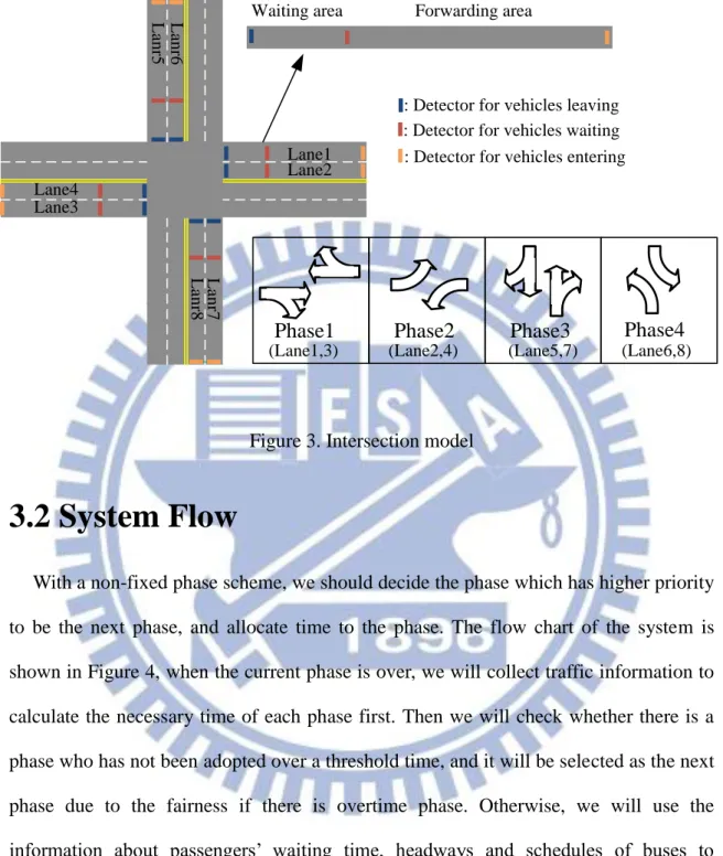
The intersection model is shown in Figure 3. Each intersection has four lanes at

each direction (west, east, north and south), two are approaching lanes, and two are

leaving lanes. The inside lane is for left-turning vehicles, and the outside lane is for

right-turning and straight-going vehicles. We install three detectors such as on each

approaching lane, and they are placing in the start, middle and end of roads to detect

number and speed of waiting vehicles, leaving vehicles and approaching vehicles. And

we divide one lane into two areas: waiting area and forwarding area. We use the vehicles

in the waiting area to determine phase length. Then we calculate passenger waiting time

will be caused by vehicles has been in the waiting area and vehicles in forwarding area

will arrive at waiting area then wait for the red signal. Then we calculate the bus

headway deviation ration and bus headway ration of buses in the waiting area. Finally,

10

: Detector for vehicles leaving : Detector for vehicles waiting : Detector for vehicles entering Waiting area Forwarding area

Phase1 Phase2 Phase3 Phase4

Lane1 Lane2 Lane4 Lane3 L an r5 L an r6 L an r7 L an r8

(Lane1,3) (Lane2,4) (Lane5,7) (Lane6,8)

Figure 3. Intersection model

3.2 System Flow

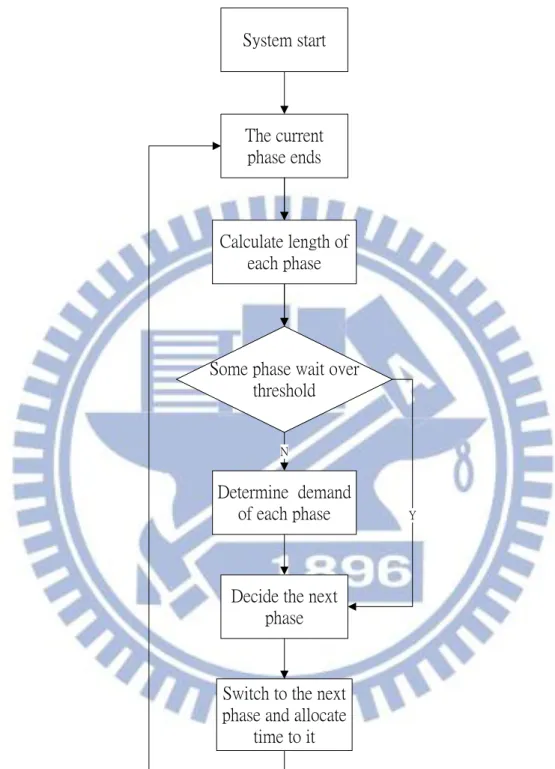
With a non-fixed phase scheme, we should decide the phase which has higher priority

to be the next phase, and allocate time to the phase. The flow chart of the system is

shown in Figure 4, when the current phase is over, we will collect traffic information to

calculate the necessary time of each phase first. Then we will check whether there is a

phase who has not been adopted over a threshold time, and it will be selected as the next

phase due to the fairness if there is overtime phase. Otherwise, we will use the

information about passengers’ waiting time, headways and schedules of buses to determine the demand of each phase. After we have the demand value of phases, we

select the phase has highest priority to be the next switch. Finally, we control the signal

11

The current phase ends

Some phase wait over threshold Calculate length of each phase Determine demand of each phase N

Decide the next phase

Y

Switch to the next phase and allocate

time to it System start

12

Chapter 4

System Design

We adopt non-fixed phase sequence to deal with the real-time changing of traffic

flow and requests of buses, so we have to determine how long each phase should be and

which phase should be selected to be next phase. The first one we can use collected data

includes location and speed of vehicles to calculate necessary time of each phase, and

introduced it more detail in section 4.1.The second one, we have to concern about

ordinary vehicles and buses, then we select three factors to design a phase demand

function. After we get the allocated time of each phase, we can calculate the first factor:

total passengers waiting time in each unit of time. Then we consider about bus regularity,

we calculate the bus schedule delay ratio and bus headway ratio to be the second and

third factor. After we calculate the phase demand value of each phase, the phase with

highest green demand value will be selected as next phase. Section 4.2 introduces the

details of phase demand determination.

4.1 Phase Length Determination

Before determining the length of each phase, we should know number of vehicles in

13

intersection only two lanes in a phase. First, we calculate the time of dispersing all

vehicles in two lanes of a phase, and we define dist( fi, ) as the distance between the

stop line and the farthest vehicle in the waiting area in the two lanes of phase f at

intersection i. An example of Phase1 is shown as see Figure 5.

Waiting area Forwarding area

…

)

,

( f

i

dist

……

Lane1 Lane3

Figure 5. Distance between stop line and the farthest vehicle of phase1

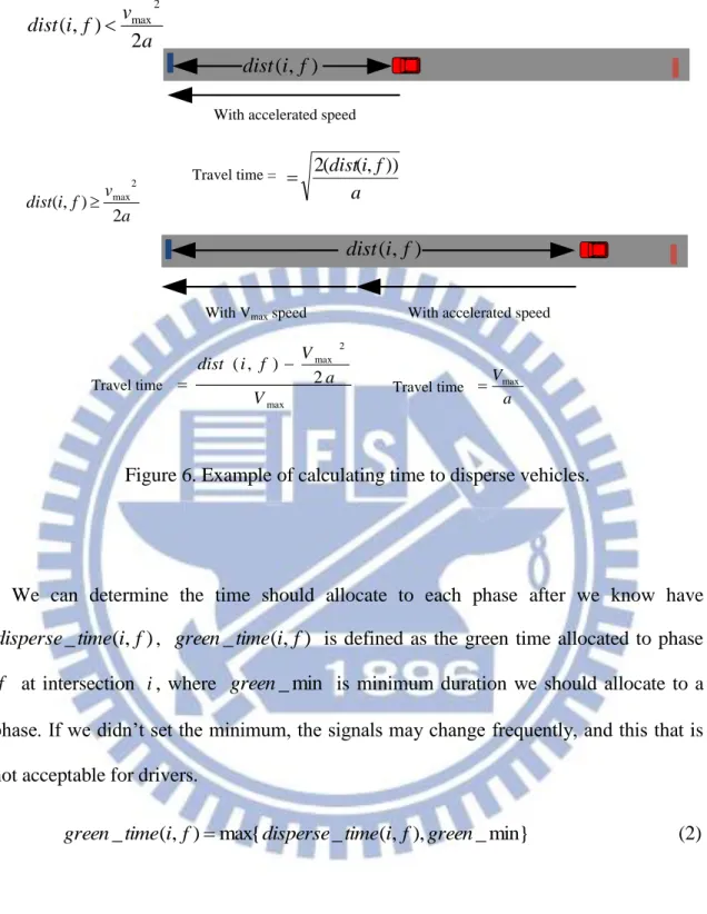
After gettingdist( fi, ), we could calculate how long can disperse the all vehicles in the waiting area of phase f . disperse_time(i,f) is defined as the time needed to

disperse all vehicles of phase f at intersection i,.Where a means the acceleration of

vehicles, and V_max means the max speed of vehicles.

          , 2 ) , ( , )) , ( ( 2 ) , ( _ max 2 max max V a V f i dist a V a f i dist f i time disperse a V f i dist if a V f i dist if 2 ) , ( 2 ) , ( 2 max 2 max   (1) When a V f i dist 2 ) , ( 2 max

 , it means that the vehicle will arrive at the stop line before it speed up to the V_max, and

a V f i dist 2 ) , ( 2 max

 means the vehicle will speed up to the V_max

and forwarding a distance at the V_max speed before it arrive at the stop line ( see Figure

14 a v f i dist 2 ) , ( 2 max  a v f i dist 2 ) , ( 2 max  ) , ( fi dist ) , ( fi dist

With accelerated speed With Vmax speed

With accelerated speed

a Vmax  max 2 max 2 ) , ( V a V f i dist   Travel time =

Travel time Travel time

a f i dist(, )) ( 2 

Figure 6. Example of calculating time to disperse vehicles.

We can determine the time should allocate to each phase after we know have

) , ( _time i f

disperse , green_time(i,f) is defined as the green time allocated to phase

f at intersection i, where green_min is minimum duration we should allocate to a phase. If we didn’t set the minimum, the signals may change frequently, and this that is not acceptable for drivers.

min} _ ), , ( _ max{ ) , (

_time i f disperse time i f green

green  (2)

4.2 Phase Demand Determination

To decide which phase should be selected, we calculate three factors including

15

phase demand function to determine the demand of each phase. And select the phase

with the highest value to be the next phase.

4.2.1 Passengers’ Waiting Time

The first factor is passengers’ waiting time, and it’s also the most evaluated item of traffic signal control systems. We calculate the total passengers’ waiting time of other

phases caused if a phase is adopting. We calculate the passengers’ waiting time of two

types of vehicles, the first type of vehicles is the vehicle in waiting area, the other type

of vehicles is the vehicle in forwarding area and will stop at waiting area for the red

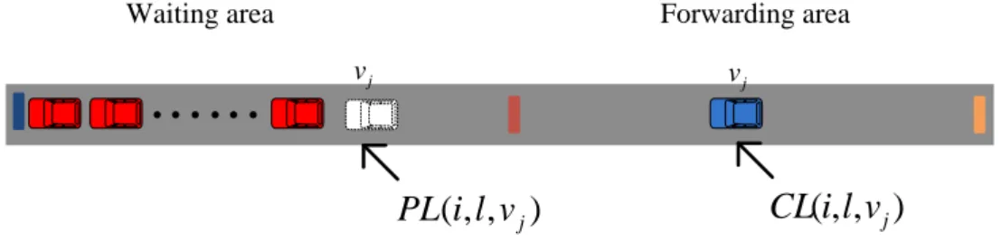
signal. To calculate the waiting of the second type, we defined CL(i,l,v_j) as the current location of the jth vehicle on lane l at intersection i, and PL(i,l,v_j) as the location of the jth vehicle will be and stop for the red signal on lane l at intersection

i.Then we can calculate the TNA(i,l,v_j) as the time needed for jth vehicle arrive at )

, , (i l v_j

PL and stop for the red signal on lane l at intersection i. The TNA(i,l,v_j) of first type of vehicles is zero because CL(i,l,v_j) is equal to PL(i,l,v_j) of these vehicles, the current location and the predicted location of the vehicle in the forwarding

area is shown as Figure 7. Where V is the current speed of v , and d is the _j deceleration of vehicles .             j j j j j j j v l i PL v l i CL if V d V v l i PL v l i CL d V v l i PL v l i CL if v l i TNA , , ( ) , , ( , 2 1 ) , , ( ) , , ( ) , , ( ) , , ( , 0 ) , , ( 2 (3)

16

……

Waiting area Forwarding area

)

,

,

(

i

l

v

_j

CL

)

,

,

(

i

l

v

_j

PL

j v j v

Figure 7. The current location and predicted location of the vehicle

Then we can calculate the waiting time of each vehicle for a time period.

) , , ( _time i f T

wait is defined as the total passengers’ waiting time if phase f sustains

for the red signal for a time period of T time, and the p(v_j) means the number of passengers on v . If the _j T is less than TNA(i,l,v_j), TTNA(i,l,v_j) would be negative, and that means the vehicle will not stop at the period of T , so the

) , , ( _time i f T

wait would be zero.





 l j j j p v v l i T N A T T f i t i m e w a i t_ (, , ) max{0,( ( , , )) ( )} ₍₄₎ An example of passengers’ waiting time cumulated by a lane is shown in Figure 8. There are i vehicles in waiting area and one vehicle in the forwarding area.

Waiting area Forwarding area

……

1 v v2 vi vi1

……

1 v v2 vi vi1

……

1 v v₂ v_i v_i1

After time, arrive at its location in waiting area

1 

i

t

At the end of the red signal

0

t

T

t

₀



1 0



t

i

t

0 _time wati 1 _timeit_i wati 1  i

v

) ( _timeiT Tti1 wati

17

Then we define wait_time(i,f) as the total passengers’ waiting time cumulated if

we allocate green_time(i,f) to phase

f

.



  _ f f f i time green f i time wait f i time wait ' )) , ( _ , ' , ( _ ) , ( _ (5)

Each phase may be allocated different length, but they may have the same

) , ( _time i f

wait  . Obviously, the phase be allocated shorter time but cause the same

total passengers’ waiting time is not effective relative to the phase has longer length. We defined wait_unit(i,f) as the total passengers’ waiting time in each unit of time if

phase f is be assigned the next phase.

) , ( _ ) , ( _ ) , ( _ f i t i m e g r e e n f i t i m e w a i t f i u n i t w a i t   (6) The previous work with non-fixed phase sequence only use the number of vehicles to

decide which phase will be assigned as the next phase and time .But they don’t concern

the waiting time cumulated by other vehicles at the period of allocated time and

passengers on each vehicle. In our traffic signal control system, we have concerned these

elements in equation (6).

In general, the phase with lower wait_unit(i,f) value will cause lower passengers’ waiting time, and the phase with higher wait_unit(i,f) will cumulate more passengers’ waiting time. If we don’t concern features of buses, we should select the phase with lower wait_unit(i,f) as the next phase, and it should have better

performance compare to the previous work.

4.2.2 Bus Schedule Delay

18

time at bus stops. The schedule of a bus route is always designed based on an ideal

experience of the bus. But because the traffic flow changes at any time, buses always

will be influenced and can’t arrive at each bus stop on the scheduled time, they may

arrive at bus stops late or early compare to its scheduled time. The buses are late from its

bus schedule should be benefited at intersections by control the traffic signal, and the

buses is early than its schedule should have lower priority at each intersection to adjust it

to close to its bus schedule.

To calculate the schedule delay, we first define schedule_arrive(i,j) _{as the time} bus j should be in phase f at intersection i, and actual_arrive(i, j)as the actual arrival

time of bus j in phase f at intersection i. Then we can calculate schedule delay of each

bus. schedule_delay(i,f) is defined as the highest schedule delay of buses in phase f

at intersection j. There may be more than one bus in the same phase at the intersection,

and they may be late or early from its schedule, but the bus with highest schedule delay

should be benefited first of all. So we select the highest schedule delay of buses in each

phase to be theschedule_delay(i,f) of phase f .

)} , , ( _ ) , , ( _ max{ ) , (

_delay i f actual arrivei f j schedule arrivei f j

schedule   (7)

4.2.3 Bus Headway Deviation

In normal situation, each bus can carry the close number of passengers and people

will not wait a bus than the headway. Although each bus departures from the first bus

stop in a fixed time interval, they may be delay or early than their predefined headway,

and it will cause people waste much time at bus stops and make some buses carry many

19

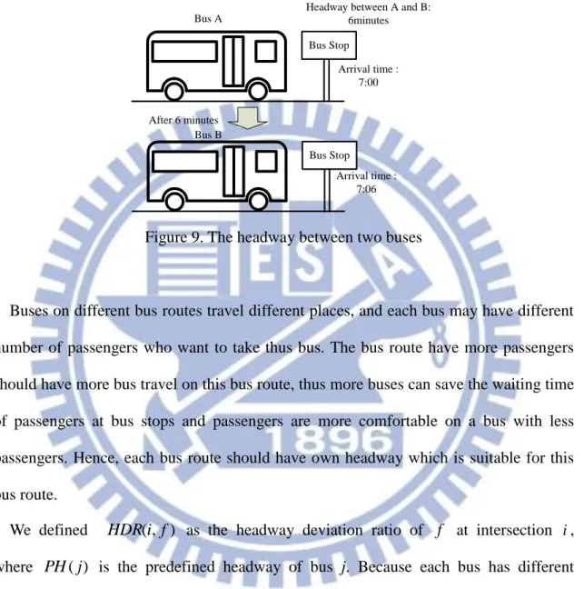
The headway between two buses is using the difference of the arrival time of the

current bus and its preceding bus. An example is shown in Figure 9. The difference of

arrival time of BusA and BusB is six minutes, and the headway is also six minutes.

Bus Stop Bus Stop Bus A Bus B After 6 minutes Arrival time : 7:00 Arrival time : 7:06

Headway between A and B: 6minutes

Figure 9. The headway between two buses

Buses on different bus routes travel different places, and each bus may have different

number of passengers who want to take thus bus. The bus route have more passengers

should have more bus travel on this bus route, thus more buses can save the waiting time

of passengers at bus stops and passengers are more comfortable on a bus with less

passengers. Hence, each bus route should have own headway which is suitable for this

bus route.

We defined HDR( fi, ) as the headway deviation ratio of f at intersection i,

where PH( j) is the predefined headway of bus j. Because each bus has different

predefined schedule, we have to use a ratio to compare headway deviation of a bus with

the other one. There may be more than one bus in the same phase at the intersection, and

the bus with highest headway deviation ratio should be benefited than buses have lower

headway deviation ratio. So we select the highest schedule delay of buses in each phase

to be HDR( fi, ) of phase f . } ) ( ) ( ) , , ( m a x { ) , ( j PH j PH f j i headway f i HDR   ₍₈₎

20

4.2.4 Phase Demand Function

Now, we define the phase demand function according to the above mentioned

measurements. In order to validate the impact from each measurement, we normalize

their domain values from zero to one. More specifically, let wait_ priority_max,

max _ _ priority

schedule and headway_ priority_max denote the maximal values

measured during the simulation, respectively. We will record the total data including

) , (

_unit i f

wait , schedule_delay(i,f) andHDR( fi, ). We set wait_ priority_max

as the two times of average value of all wait_unit(i,f) , and we set

max _ _ priority

schedule and headway_ priority_max the same way.

Then we define wait_priority(i,f) , schedule_priority(i,f) and

) , ( _priority i f headway . _ _m a x ) , ( _ ) , ( _ p r i o r i t y w a i t f i u n i t w a i t f i p r i o r i t y w a i t  , (9) _ _max ) , ( _ ) , ( _ priority schedule f i delay schedule f i priority schedule  (10) _ _m a x ) , ( ) , ( _ p r i o r i t y h e a d w a y f i HDR f i priority headway  . (11)9

Besides, we give three scaling factors



₁,



₂and



3 denote as the weight of

passenger waiting time, bus schedule delay ratio and bus headway deviation ratio. The

21 ) , ( _ ) , ( _ ) , ( _ ) ( ) , ( _ 3 2 1 f i priority headway f i priority schedule f i priority wait f i demand phase           (12)

At each intersection, if there is an overtime phase, the overtime phase will be selected.

22

Chapter 5

Simulation

In this section, we evaluate the performance of ATCB by using NetLogo simulator

[23] (version 4.1.3). We compare ATCB with the traditional predefined fixed-time

scheme with bus priority strategy like TDTSP [19] and an adaptive fuzzy logic control

(AFLC) [21].Beside bus priority, we also compare ATCB with an actuated traffic control

and a non-fixed sequence control scheme [10]. The details of each scheme are described

below.

We modify the TDTSP: We use a fixed sequence traffic signal control scheme and

we benefit bus by extending the current phase if there is a bus can pass through the

intersection by the current phase. If there are two buses on different routes meet in an

intersection, we compare the headway deviation and schedule delay to decide which bus

will be benefits.

Then, we modify AFLC: Like TDTSP, we also adopt a fixed sequence traffic signal

control scheme and decide whether to extend the current phase or switch to next phase.

In our modification, we compare ordinary vehicles and buses of the current phase with

ordinary vehicles and buses of the next phase to decide whether to extend the current

phase or switch to the next phase.

Actuated traffic control method controls signals by detecting the coming vehicles.

23

vehicles will cross the intersection in a short period, it will extend the current phase until

reach its maximum green time.

In a non-fixed sequence scheme, when the current phase is going to end, it will find

the most suitable phase from all phases, the original scheme consider many factors, in

our modification, we only focus on the number of vehicles, the phase has the biggest

number of vehicles will be selected as the next phase.

We analyze the simulation results of total waiting time of vehicles, total waiting

time of buses, total passengers’ waiting time, average bus schedule deviation and average bus headway deviation.

5.1 Simulation Environment

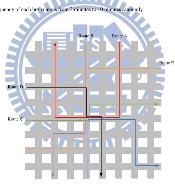
As shown in Figure 10, we perform the simulation on a network of 8×8 traditional four-direction intersections, and the length of roads is 500 meters. The length of the

waiting area on each road is 200 meters, and each road has four lanes, two are

approaching lanes, and two are leaving lanes. We generate the ordinary vehicles on the

edge roads of the network in a rate of 10 vehicles/minutes. Each vehicle are created with

a speed of 14m/s. The acceleration of vehicles is assigned as 2m/s2, it means that each vehicle will reach its limit speed in 7 second. The deceleration of vehicles is 4m/ s2. Each vehicle will keep a safe distance when it is driven. And we adopt each vehicle

carry average two passengers. In this network, we set five bus routes (RouteA, RouteB,

RouteC, RouteD and RouteE), each bus on different bus routes enter this map with

different frequencies (predefined headway). And we let them meet at an intersection to

generate a pivot intersection, the bus routes is shown in Figures 10. And passengers on

24

detail parameter of simulation is shown in TABLE 1.

We generate these five routes randomly. First, we randomly select a pivot

intersection, and the distance between the pivot intersection and edges of this map is at

least two intersections. For each route, we give an entry and an exit randomly, and the

entry can’t be also the exit. The buses of the route will pass through the pivot

intersection, if the route is illegal or the length of this route is less than eight

intersections, we will generate a new route until the route is legal and enough long. The

frequency of each bus route is from 3 minutes to 10 minutes randomly.

Route A Route B Route C Route D Route C Route E

25

Table 1. Simulation parameters

Map size 8*8 grid

Length of roads 500 m

Length of waiting area 200 m

Traffic flow the edge road 10 vehicles/min

Speed limit 14 m/s (50 km/h) Acceleration 2 m/s2 deceleration 4 m/s2 Passengers of a ordinary vehicle 2 Passengers of a bus 10~20 Run time 2h

Route A predefined headway 3~10 min

Route B predefined headway 3~10 min

Route C predefined headway 3~10 min

Route D predefined headway 3~10 min

26

5.2 Simulation Results

In the preliminary experiment, we fine the appropriate value of each weight (₁:0.5,

2

 :0.5, ₃:0.75) to reduce the headway deviation and schedule delay of buses and

don’t produce huge impact on the passengers’ waiting time. And we use these value in the below simulation.

We first evaluate the waiting time of buses in ATCB and other control strategies,

which is the sum of waiting time at intersection of all buses. Figure 11 is the result of

total waiting of all buses, and it shows that our scheme ATCB has the best performance

at reducing bus waiting time, and it is better than other methods at least 40 percent. Both

TDTSP and ADT consider bus priority which extends its current phase, the former one

considers headway deviation, and the later one considers both the ordinary vehicles and

buses. They have better performance than the actuated scheme which doesn’t consider

bus priority. The non-fixed phase scheme doesn’t consider bus priority, but the non-fixed

scheme is better than actual due to it is better for all vehicles include buses and ordinary

vehicles.

Figure 11. Total waiting time of buses

0 20 40 60 80 100 120 0 1 2 3 4 5 6 7 8 9 10x 10 4 Time (min) T o ta l w a it in g t im e ( s e c ) ATCBTDTSP Actuated AFLC Non-fixed

27

Table 2. Total waiting time of buses and average waiting time of each bus in one intersection

Scheme Total waiting time in

two hours

Average waiting time of each

bus in one intersection

ATCB 3.79 × 104 sec 12.31 sec

TDTSP 7.04 × 104 sec 22.57 sec

Actuated 8.79 × 104 sec 28.04 sec

AFLC 6.71 × 104 sec 21.72 sec

Non-fixed 6.38 × 104 sec 20.66 sec

We could see that the best performance is non-fixed scheme, since that the non-fixed

scheme don’t concern bus priority. And our ATCB concern bus priority from bus schedule delay, headway deviation, number of passengers so our total waiting time of all

vehicles is more than the non-fixed scheme. But the difference is just 3.8 percent, and it

is acceptable because we can save 40 percent waiting time of buses as shown in Figure

11. And TDTSP has the poor performance due to that it doesn’t concern the real-time

information except bus information. Actuated scheme extends the current phase to

permit vehicles pass through intersections is more better than TDTSP due to that it can

avoid vehicles wasting a lot of time waiting for signals just because it misses few

28

Figure 12. Total waiting time of vehicles

Table 3. Total Waiting time of buses and average waiting time of each vehicle in one intersection

Scheme Total waiting time in

two hours

Average waiting time of each

vehicle in one intersection

ATCB 1.47 × 107 sec 25.95 sec

TDTSP 2.23 × 107 sec 38.11 sec

Actuated 1.55 × 107 sec 26.78 sec

AFLC 1.61 × 107 sec 27.26 sec

Non-fixed 1.42 × 107 sec 24.67 sec

The passenger’s total waiting time is shown in Figure 13. And we could find that the result shown in Figure 13 is similar to Figure 12, but the performance of our ATCB is

better than the non-fixed phase scheme, because we consider the number of passenger of

each vehicle in our equation (5). If we don’t consider number of passengers of each vehicles like non-fixed phase scheme, the bus will be treated as ordinary vehicle without

0 20 40 60 80 100 120 0 0.5 1 1.5 2 2.5x 10 7

Time (min)

T

o

ta

l

w

a

it

in

g

t

im

e

(

s

e

c

)

ATCBTDTSP Actuated AFLC Non-fixed

29

bus priority. And we could see it has better performance of ordinary vehicles as shown in

Figure 12, but it has poor performance in the result of passengers’ waiting time.

Figure 13. Total waiting time of passengers

Table 4. Total waiting time of passengers and Average waiting time of each vehicle in one intersection

Scheme Total waiting time in two hours

Average waiting time of each passenger in one intersection

ATCB 1.50 × 107 sec 24.32 sec

TDTSP 2.28 × 107 sec 36.96 sec

Actuated 1.61 × 107 sec 26.10 sec

AFLC 1.66 × 107 sec 26.91 sec

Non-fixed 1.46 × 107 sec 23.67 sec

Then we evaluate the schedule delay of buses. We need buses travel a distance to

produce bus schedule delay, so we collect the information from pivot intersection, and

this intersection is a congested intersection because it is passed through by buses of all

bus routes. As shown in Figure 14 and Table 5, we record 30 records of the schedule

0 20 40 60 80 100 120 0 0.5 1 1.5 2 2.5x 10 7

Time (min)

T

o

ta

l

w

a

it

in

g

t

im

e

(

s

e

c

)

ATCB_TDTSP Actuated AFLC Non-fixed

30

delay of buses on RouteA when it arrives at this intersection. We could find that our

ATCB has a lowest average schedule delay, which is better at least 25 percent than other

schemes. The variance of bus schedule delay of ATCB is 337.79, and it is better than

other schemes at least 63.7 percent.

Figure 14. Bus schedule delay in a bus stop at a pivot intersection

Table 5. Average schedule delay time and Variances of buses at a pivot intersection

Scheme Average schedule delay time Variances of bus schedule delay

ATCB 30.87 sec 337.79 sec

TDTSP 46.88 sec 930.52 sec

Actuated 47.77 sec 1360.84 sec

AFLC 57.22 sec 1971.85 sec

Non-fixed 55.80 sec 985.0 sec

5 10 15 20 25 30 0 20 40 60 80 100 120 140 160 180 Bus (veh) B u s d e la y ( s e c ) ATCB TDTSP Actuated AFLC Non-fixed

31

As shown in Figure 15 and Table 5, we evaluate headway deviation of buses. We still

collect records of bus headway deviation ratio at the pivot intersection. As shown in

Figure 14 and Table 5, in ATCB, the average bus headway deviation ratio is 22.19

percent, and the range of bus headway deviation ratio is from -44 percent to 39 percent

and variance is 601.54 percent. The second best performance is TDTSP, and its average

bus headway deviation ratio is 22.19 percent, and the range of bus headway deviation

ratio is from -68 percent to 70 percent and variance is 601.54 percent.

We also evaluate the total schedule delay time and bus headway deviation ratio which

is shown in Table 7, and the result is similar to the result shown in Table5 and Table6.

Our ATCB still have the best performance.

Figure 15. Bus headway deviation ratio in a bus stop at a pivot intersection

5 10 15 20 25 30 -80 -60 -40 -20 0 20 40 60 80 100 120 Bus (veh) B u s d e v ia ti o n r a ti o ( % ) ATCB TDTSP Actuated AFLC Non-fixed

32

Table 6. Average headway deviation ratio and variances of buses at a pivot

intersection

Scheme Average headway

deviation ratio

Variances of bus headway

deviation ratio ATCB 19.19 % 601.54 TDTSP 35.16 % 1105.39 Actuated 49.39 % 2215.51 AFLC 54.35 % 2603.06 Non-fixed 37.54 % 1681

Table 7. Simulation result

Scheme Total waiting time of buses Total waiting time of vehicles Total waiting time of passengers Average schedule delay Average headway deviation ratio ATCB 3.79 × 104 sec 1.47 × 107 sec 1.50 × 107 sec 38.27 sec 29.21 % TDTSP 7.04 × 104 sec 2.23 × 107 sec 2.28 × 107 sec 46.32 sec 35.01 % Actuated 8.79 × 104 sec 1.55 × 107 sec 1.61 × 107 sec 55.21 sec 43.12 % AFLC 6.71 × 104 sec 1.61 × 107 sec 1.66 × 107 sec 53.92 sec 42.22 % Non-fixed 6.38 × 104 sec 1.42 × 107 sec 1.46 × 107 sec 54.25 sec 38.56 %

33

5.3 A Simulation in Real Urban Environment

To prove ATCB is still effective in real world, we have designed a road network of Taipei City in Taiwan, a rough map is shown in Figure 16. This network has 16

intersections. And we have select 5 real bus routes to simulate.

The result is shown in Table 8, and we can find that the result is similar to the performance in Table 7, that can prove our method ATCB is still effective in a real road network. But because the size of this map is small, so the benefits of reducing waiting of buses are more obvious than the benefits of buses headway and bus schedule than the result of the bigger map.

Shimin Blvd Zhongxiao East Rd Renai Rd Xinyi Rd G u an g fu S o u th R d D u n h u a S o u th R d F u x in g S o u th R d Ji an g u o S o u th R d

34

Table 8. Simulation result of a real urban environment

Scheme Total waiting time of buses Total waiting time of vehicles Total waiting time of passengers Average schedule delay Average headway deviation ratio ATCB 3.84 × 103 sec 2.54 × 106 sec 2.57 × 106 sec 19.12 sec 25.31 % TDTSP 1.25 × 104 sec 4.35 × 106 sec 4.44 × 106 sec 22.23 sec 31.60 % Actuated 1.43 × 104 sec 2.78 × 106 sec 2.89 × 106 sec 28.78 sec 39.53 % AFLC 1.33 × 104 sec 2.85 × 106 sec 2.95 × 106 sec 27.15 sec 34.51 % Non-fixed 1.15 × 104 sec 2.45× 106 sec 2.53× 106 sec 24.74 sec 33.49 %

35

Chapter 6

Conclusion

In this paper, the adaptive traffic signal control system (ATCB) has been proposed for

ordinary vehicles and buses in urban environment. We adopt non-fixed phase scheme,

and we use collected traffic information from detectors on roads and buses to determine

the next phase and the phase should be allocated. To determine which phase is suitable

to be adopted, we concern the passengers’ waiting time and bus priority which include

bus headway deviation and bus schedule delay to determine the demand of each phase.

And the phase which cause lowest passengers’ waiting and improve schedule delay and headway deviation will be selected. The simulation results show that ATCB performs

better at reducing passenger’s waiting time at least 40 percent, and improving schedule

delay at least 17.5 percent, and headway deviation of buses at least 6 percent.

For the future works, the prediction model of traffic flow is also an important point in

traffic signal control systems, and we could have better performance by implementing

the prediction model of traffic flow in our system. Furthermore, we will try to use the

36

References

.

[1] D. I. Robertson and R. D. Bretherton, “Optimizing networks of trafficsignals in real

timełthe scoot method,” IEEE Transactions on Vehicular Technology,vol. 40, no. 3, pp. 11–15, 1991.

[2] A. G. Sims and K. W. Dobinson, “The sydney coordinated adaptive traffic (scat)

system philosophy and benefits,” IEEE Transactions on Vehicle Technology, vol.

29, no. 2, pp. 130–137, 1980.

[3] E. Y. Luz and A. Mimbela “A summary of vehicle detection and surveillance

technologies use in intelligent transportation systems.” http://www.nmsu.edu/~traffic/

[4] B. Zhou, J. Cao, X. Zeng, and H. Wu, “Adaptive Traffic Light Control in Wireless

Sensor Network-Based Intelligent Transportation System,” IEEE Conference on

Vehicular Technology, pp1-5 May 2010.

[5] N. Maslekar, M. Boussedjra, J. Mouzna, and H. Labiod,“VANET Based Adaptive

Traffic Signal Control.” IEEE Conference on Vehicular Technology, pp. 1-5, 2011.

[6] I. Arel, C. Liu, T. Urbanik, and A. Kohls, “Reinforcement learning-based

multi-agent system for network traffic signal control,” IET Intelligent Transport

Systems, vol. 4, no. 2, pp. 128–135, 2010.

[7] A. Guerrero-Ibanez, J. Contreras-Castillo, R. Buenrostro, A. B. Marti, and A. R.

37

traffic-light control”, IEEE Intelligent Vehicles Symposium, pp. 694-696, June

2010.

[8] K. Mizuno, Y. Fukui, S. Nishihara, “Urban Traffic Signal Control Based on

Distributed Constraint Satisfaction,” Hawaii International Conference on System

Sciences, pp. 65, 2008.

[9] T. Li, D. Zhao, and J. Yi, “Adaptive Dynamic Programming for Multi-intersections

Traffic Signal Intelligent Control,” IEEE Conference on Intelligent Transportation Systems, pp. 286-291, 2008.

[10] B. Zhou, J. Cao, H. Wu, “Adaptive Traffic Light Control of Multiple Intersections

in WSN-based ITS”, IEEE Conference on Vehicular Technology, pp15-18 May

2011.

[11] T. H. Heung, T. K. Ho, and Y. F. Fung, “Coordinated road-junction traffic control

by dynamic programming,” IEEE Transactions on Intelligent Transportation Systems, vol. 6, no. 3, pp. 341–350, Sep. 2005.

[12] P. B. Mirchandani and F.-Y. Wang, “RHODES to intelligent transportation

systems,” IEEE Intell. Syst., vol. 20, no. 1, pp. 10–15, Jan./Feb. 2005.

[13] T. H. Heung, T. K. Ho, and Y. F. Fung, “Coordinated road-junction traffic control

by dynamic programming,” IEEE Transactions on Intelligent Systems, vol. 6, no. 3, pp. 341–350, Sep. 2005.

[14] Y. W. Kim, T. Kato, S. Okuma, and T. Narikiyo, “Traffic network control based on

hybrid dynamical system modeling and mixed integer nonlinear programming with

convexity analysis,” IEEE Transactions on Systems, Man and Cybernetics, vol. 38, no. 2, pp. 346–357, Mar. 2008.

38

[15] Y. S. Murat and E. Gedizlioglu, “A fuzzy logic multi-phased signal control model

for isolated junctions,” Transportation Research Part C: Emerging Technologies, pp. 19–36, 2005.

[16] D. Srinivasan, M. C. Choy, and R. L. Cheu, “Neural networks for realtime traffic

signal control,” IEEE Transactions on Intelligent Systems., vol. 7, no. 3, pp. 261–272, Sep. 2006.

[17] J. D. Schmocker, S. Ahuja, and M. G. H. Bell, “Multi-objective signal control of

urban junctions—Framework and a London case study,” Transportation Research

Part C: Emerging Technologies, pp. 454–470, 2008.

[18] N. Hounsell, B. Shrestha, J. Head, S. Palmer, and T. Bowen, “The way ahead for

London’s bus priority at traffic signals,” IET Intelligent Transport Systems, vol. 2, no. 3, pp. 193–200, Sep. 2008.

[19] W. Ma, X.Yang, “Design and Evaluatio Priority System Base on Wireless Sensor

Network”, IEEE conference on Intelligent Transportation Systems, pp. 1073-1077,Sep2008.

[20] Bhouri, N.; Haciane, S.; Balbo, F., “A Multi-Agent System to Regulate Urban

Traffic: Private Vehicles and Public Transport”, International IEEE conference on Intelligent Transportation Systems, pp1575-1581,2010.

[21] G. J. Shen and X. J. Kong, “Study on road network traffic coordination control

technique with bus priority,” IEEE Transactions on Systems, Man and Cybernetics, vol. 39, no. 3, pp. 343–351, May 2009.

[22] Hounsell, N.; Shrestha, B., “A New Approach for Co-Operative Bus Priority at

Traffic Signals,” IEEE Transactions on Intelligent Transportation Systems, vol. 13, no. 1, pp. 6–14, Sep. 2005.

39

[23] Wilensky, U. NetLogo (and NetLogo User Manual), Center for Connected

Learning and Computer-Based Modeling, Northwestern University.