從蛋白質序列預測殘基相對溶劑可接觸性

全文

(1)國立交通大學生物資訊研究所碩士論文. 從蛋白質序列預測殘基相對溶劑可接觸性 Prediction of Protein Relative Solvent Accessibility from Amino Acid Sequence. 研究生：徐蔚倫指導教授：黃鎮剛. 教授. 中華民國九十四年七月.

(2) 從蛋白質序列預測殘基相對溶劑可接觸性 Prediction of Protein Relative Solvent Accessibility from Amino Acid Sequence. 研究生：徐蔚倫. Student：Wei-Lun Hsu. 指導教授：黃鎮剛. Advisor：Jenn-Kang Hwang. 國立交通大學生物資訊研究所碩士論文. A Thesis Submitted to Institute of Bioinformatics College of Biological Science and Technology National Chiao Tung University in partial Fulfillment of the Requirements for the Degree of Master In. Bioinformatics. July 2005. Hsinchu, Taiwan, Republic of China. 中華民國九十四年七月.

(3) 從蛋白質序列預測殘基相對溶劑可接觸性. 學生：徐蔚倫. 指導教授：黃鎮剛國立交通大學生物資訊研究所碩士班. 中文摘要. 從序列資訊來預測蛋白質三級結構是目前生物學研究上非常重要的目標之一，而正確的預測蛋白質相對溶劑可接觸性則可以提供蛋白質三級結構相關的資訊。蛋白質相對溶劑可接觸性(RSA)代表著蛋白質上某一個氨基酸和溶劑接觸的程度。通常蛋白質的結合處會位於它的表面，因此，若能正確的預測蛋白質位於表面的氨基酸位置，就能夠更進一步的瞭解該蛋白質的功能。此外，一個蛋白質位於表面和包埋在蛋白質內部的氨基酸分佈，也被觀察到和蛋白質在細胞內的位置有很大的關連性。我的方法是利用支持向量機將局部和整體的蛋白質資訊，其中最好的結果是利用位置加權矩陣(PSSM)、二級結構特徵值(secondary structure profile)和氨基酸親水程度(hydropathy indexes)作為輸入向量。這個方法對於 RS126 資料群在以 25%為分類閾值時，可以達到 77.2%，和最近幾年的在這方面的研究成果 75%-78.3%達到相近的程度，而在將 RSA 分成十類的預測結果中也可達到 15.2% 平均絕對誤差，預測值和實驗值達到 0.51 的相關性。. i.

(4) Prediction of Protein Relative Solvent Accessibility from Amino Acid Sequence Student：Wei-Lun Hsu. Advisor：Jenn-Kang Hwang. Institute of Bioinformatics, National Chiao Tung University. Abstract. The prediction of the three-dimensional structure from its sequence is probably one of the most important goals of modern biology. The accurate prediction of protein relative solvent accessibility is useful for the prediction of tertiary structure of a protein. Amino acid solvent accessibility is the degree to which a residue in a protein is accessible to a solvent molecule. Because the binding sites of a protein are usually located on its surface, accurately predicting the surface residues can be regarded as an important step toward determining its function. On the other hand, it has been observed that the distribution of surface residues of a protein is correlated with its subcellular environments; consequently, information of surface residues may improve the prediction of protein subcellular localization. Presently, out best method is based on the support vector machines using as the input feature vectors, the sliding window that includes the local environment descriptors such as PSSM, secondary structure profile and hydropathy indexes. In my work, relative solvent accessibility based on a 2-state model, for 25%, 16%, 5%, and 0% accessibility are predicted at 77.2%, 77.1%, 80.4%, and 88.4% accuracy, respectively. Furthermore, solvent accessibility prediction methods have in recent years reached accuracy in the range of 75.0-78.3% at 25% threshold. And the results based in a 10-state model can reach 15.2% mean absolute error and 0.51 correlations.. ii.

(5) 誌謝在求知的路上總是要一直不斷的經歷各種學習的過程，才能不斷的成長進步。在研究所二年的時間裡，各方面我都是收穫良多，真的很慶幸能身處在這樣一個優質的學習環境中體驗研究生生活。. 首先，很感謝我的指導教授黃鎮剛老師，帶領我進入研究的領域，不但提供我們一個良好獨立的研究環境，更不斷的在我研究遇到問題、瓶頸時，給予我適當的建議與協助。在老師身上，我學習到的不只是研究方面的知識和方法，更重要的是一個學者對求知的熱誠和執著態度。. 另外，也很謝謝實驗室的夥伴們，除了生活上的彼此協助照應、精神上的鼓勵之外，很多研究上的問題也是透過大家的討論和互相協助，才能夠順利的解決，讓我的研究能如期完成。. 最後，我也要感謝我的家人，在我求學路上，一直全力支持我，讓我能夠在研究上全力以赴、順利完成學業。僅以此論文作為我碩士研究生涯的總結，並將此獻給所有關心我及我所誠摯感謝的人。. iii.

(6) 目錄. 中文摘要 ………………………………………………………………………………. i. 英文摘要. ……………………………………………………………………………… ii. 誌謝. ……………………………………………………………………………… iii. 目錄. ……………………………………………………………………………… iv. 表目錄. ……………………………………………………………………………… vi. 圖目錄. ……………………………………………………………………………… vii. 1.. Introduction …………………………………………………………………. 1. 2.. Material and Methods ………………………………………………………. 3. 2.1. Definition and thresholds of solvent accessibility …………………………. 3. 2.2. Training and data sets ………………………………………………………. 4. 2.3. Feature vectors ………………………………………………………………. 4. 2.3.1. Local descriptors ……………………………………………………………. 4. 2.3.1.1. PSSM (position-specific scoring matrices) …………………………………. 5. 2.3.1.2. Secondary structure profiles…………………………………………………. 5. 2.3.1.3. Hydropathy indexes …………………………………………………………. 5. 2.3.1.4. Amino acid in binary coding…………………………………………………. 6. 2.3.1.5. Amino acid properties in binary coding ……………………………………. 6. 2.3.1.6. Local amino acid composition ………………………………………………. 6. 2.3.1.7. Local amino acid properties composition……………………………………. 6. 2.3.1.8. Residue size …………………………………………………………………. 6. 2.3.2. Global descriptors……………………………………………………………. 7. 2.3.2.1. Global amino acid composition ……………………………………………. 7. 2.3.2.2. Global amino acid properties composition …………………………………. 7. 2.4. Performance measures………………………………………………………·. 7. 2.4.1. In 2-state prediction and 3-state prediction …………………………………. 7. 2.4.2. In 10-state prediction………………………………………………………··. 8. iv.

(7) 2.5. Support vector machine ……………………………………………………. 8. 3.. Server Development and Administration System Overview ……………… 10. 4.. World Wide Web Interface ………………………………………………… 11 4.1. Models trained by the three benchmark data sets…………………………… 11. 4.2. Models of different state thresholds………………………………………… 11. 4.3. Query sequence ………………………………………………………·…… 11. 4.4. Website ……………………………………………………………………·· 11. 5.. Results and Discussion……………………………………………………… 12 5.1. Prediction accuracies and MCC values using individual local descriptors with RS126 dataset in 2-state prediction model …………………………… 12. 5.2. Prediction accuracies and MCC values using comprehensive local descriptors with RS126 dataset in 2-state prediction model………………… 12. 5.3. Prediction accuracies and MCC values of the benchmark test on the RS126, NM215 and KP480 datasets in 2-state prediction model and its comparison with other methods ………………………………………………………… 13. 5.4. MAE and Pearson’s “r” values of the benchmark test on the RS126 and KP480 datasets in 10-state prediction model ……………………………… 13. 6.. Conclusion ………………………………………………………………… 15. 參考文獻 ………………………………………………………··……··………··……… 43. v.

(8) 圖目錄 Figure 1. An outline of the PSSM input vectors, which shows how the PSI-BLAST score matrices are processed……………………………………………… 16. Figure 2. The input vectors called “secondary structure profiles”…………………. 17. Figure 3. The input vectors called “hydropathy indexes” ………………………… 18. Figure 4. The input vectors called “amino acid in binary coding” ………………… 19. Figure 5. The input vectors called “amino acid properties in binary coding”……… 20. Figure 6. The input vectors called “local amino acid composition”………………… 21. Figure 7. The input vectors called “local amino acid properties composition” …… 22. Figure 8. The input vectors called “residue size”. Figure 9. The input vectors called “global amino acid composition” ……………… 24. Figure 10. The input vectors called “global amino acid properties composition” … 25. Figure 11. The figure shows the components of SAS prediction server, and most of. ………………………………… 23. the connection was built using the Perl language and CGI package……… 26 Figure 12. The World Wide Web interface of the RSA prediction server…………… 27. Figure 13. The standard output webpage of prediction ……………………………… 28. vi.

(9) 表目錄 Table 1. Maximum value of solvent accessible surface areas of each kind of residue calculated by MOLSIM program…………………………………………… 29. Table 2. The RS126 dataset used in this study ……………………………………… 30. Table 3. The NM215 dataset used in this study……………………………………… 31. Table 4. The KP480 dataset used in this study ……………………………………… 32. Table 5. The hydropathy index of the standard amino acids………………………… 35. Table 6. The classification of the standard amino acids by R groups………………… 36. Table 7. Prediction accuracies and MCC values using individual local descriptors with RS126 datasets in 2-state prediction model…………………………… 37. Table 8. Prediction accuracies and MCC values using comprehensive local descriptors with RS126 datasets in 2-state prediction model ……………… 38. Table 9. Prediction accuracies of the benchmark tests on the RS126, NM215 and KP480 datasets in 2-state prediction model and its comparison with other methods……………………………………………………………………… 39. Table 10. MCC values of the benchmark tests on the RS126, NM215 and KP480 datasets in 2-state prediction model and its comparison with other methods……………………………………………………………………… 40. Table 11. MAE and Pearson's "r" values of the benchmark tests on the RS126 and KP480 datasets in 10-state prediction model ……………………………… 41. vii.

(10) 1. Introduction Knowledge of protein’s three-dimensional (3D) structure is essential for a full understanding of its functionality. However, only a small fraction of the enormous number of sequenced proteins has their structure determined. In order to reduce the gap between sequence and structure, developing reliable and applicable structure prediction methods has become a more important task in computational biology. Thus simplification of the problem from 3D structures to 1D feature may be useful as a first-step. The relative solvent accessibility of an amino acid in protein is a real value that represents the solvent exposed surface area of this residue in relative terms. The prediction of secondary structure is more familiar and well-defined aspect of the problem and the prediction of residue solvent accessibility is another aspect. Secondary structures and solvent accessibilities of amino acid residues give a useful insight into the structure and function of a protein. In particular, the knowledge of solvent accessibility has assisted alignments in regions of remote sequence identity for threading. In addition to providing insight into the conformation of 3D structure, prediction of residue solvent accessibility has many other applications. For example, it has been observed that the distribution of surface residues of a protein is correlated with its subcellular environment. Many studies[1] have suggested that hydrophobic core residues are likely sites of deleterious mutations. The residues in site of deleterious mutations may be critical for protein stability. Wang and Molt[2] found that the vast majority of disease mutations affected protein stability rather than function and could be predicted using straightforward rules. There are various approaches have been developed, typically by examining a window of residues centered at the test residue and using sequence input or sequence profile as input vectors. These include neural network[3-7], Bayesian statistics[8], linear regressions[9, 10],. -1-.

(11) information theory[11], support vector machines[12, 13] and fuzzy k-nearest neighbor method[14]. However, in contract to the secondary structure, there is no widely accepted criterion for classifying the experimentally determined solvent accessibility into a finite number of discrete states such as buried, intermediate and exposed states. Also, the prediction accuracies of solvent accessibility are lower than those for secondary structure prediction, since the solvent accessibility is less conserved than secondary structure[3], although there has been some progress recently. In this work, relative solvent accessibility based on a 2-state model in RS126 dataset, for 25%, 16%, 5%, and 0% accessibility are predicted at 77.2%, 77.1%, 80.4%, and 88.4% accuracy, respectively. And the results based in a 10-state model can reach 15.2% mean absolute error and 0.51 correlations.. -2-.

(12) 2. Material and Methods 2.1 Definition and thresholds of solvent accessibility. The relative solvent accessibility of an amino acid is the degree that present the residue in a protein is accessible to solvent molecules. The relative solvent accessibility can be calculated by the formula as follows,. Re lACC = 100 ⋅. ACC MaxACC. (1). RelACC : relative solvent accessibility ACC : solvent accessible surface areas MaxACC : maximum value of solvent accessible surface areas of each kind of residue. Where ACC of ith residue is the solvent accessible surface areas calculated by the dictionary of protein secondary structure program (DSSP) [15], and the MaxACC are taken from MOLSIM program (Table 1). RelACC is derived from normalizing ACC by dividing the DSSP. accessibility by the maximum accessibility of amino acid residues corresponding to accessibility for a Gly-X-Gly extended tripeptide conformation. RelACC can hence adopt values between 0% and 100%, with 0% corresponding to a fully buried and 100% to a fully accessible residue, respectively.. Various thresholds have been used to classify residues as buried and exposed (2-state prediction) or buried, intermediate and exposed (3-state prediction) in previously published results. In this work, thresholds of 0, 5, 16, 25% for buried/exposed in the 2-state predictions, thresholds of 9, 36% for buried/intermediate/exposed in the 3-state predictions and 10, 20, 30, 40, 50, 60, 70, 80, 90% for classifying residues in 10 classes are used.. -3-.

(13) 2.2 Training and data sets. The solvent accessibility was predicted for three sets of proteins in order to evaluate the performance of our method. They are a 126-protein dataset of Rost and Sander[3] (Table 2), a set of 215 protein chains selected by Naderi-Manesh[11] (Table 3), and 480 proteins from Kim and Park[13] (Table 4). Each of these data sets consists of protein sequence with less than 25% homology. To perform 7-fold cross validation test, we randomly divided these data sets into 7 groups, each containing a roughly equal number of protein sequences. One group was chosen as the testing set, while others were merged into the training set.. 2.3 Feature vectors. In the first phase, we have individually benchmarked 8 different local descriptor types in prediction experiment in RS126 dataset. Our results revealed that the five best-performing sets of local descriptors were using PSSM (position-specific scoring matrices), secondary structure profiles, hydropathy indexes, amino acid composition and amino acid properties by their R groups. In second phase, the five top-performing local descriptors were combined to obtain a new method with improved performance. And then, we add 2 different global descriptors types into the method to see if global descriptors are useful for solvent accessibility prediction.. 2.3.1 Local descriptors. We represent the local environment of sequences by using sliding window coding scheme. Increasing the window size can provide more local information and it is reasonable to expect that prediction accuracy would increase with the enlargement of the window size. But the past research[12] found that window size has a very limited effect on prediction accuracy.. -4-.

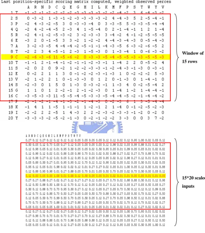
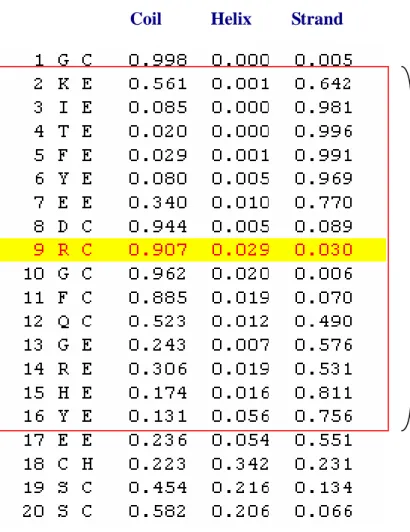
(14) Therefore, we followed the paper and selected 15 for the window size for the prediction of protein relative solvent accessibility. 2.3.1.1 PSSM (position-specific scoring matrices). We use PSI-BLAST[16] against non-redundant protein sequence database for 5 iterations to produce PSSM, which has 20*m elements, where m is the length of query sequences and each element represents the log-likelihood of that specific residue substitution at that position in the template (based on a weighted average of BLOSUM62 matrix scores for the given alignment position). PSI-BLAST uses a simple but effective scheme for weighting the contribution of locally different numbers of sequences to the resulting profiles. The profile matrix elements are scaled to the required 0-1 range by using the standard logistic function as below, where x of the equation is the raw profile matrix value.. Score =. 1 1 + e−x. (2). Then, the input vector has 20*15 components (Illustrated in Figure 1). Each component can be expressed as PSSMijk, where i is the predicted residue, j is the location in the sliding window and k is the type of amino acid.. 2.3.1.2 Secondary structure profiles. The secondary structure profile has 3*m elements. The elements describe the probabilities of each residue in the three kinds of secondary structures which are Helix, Sheet and Coil. These profiles were generated from the PSIPRED[17] program, and each input vector has 3*15 components (Illustrated. in Figure 2). Each component can be expressed as SSijk, where i is the predicted residue, j is the location in the sliding window and k is the type of secondary structure including helix, -5-.

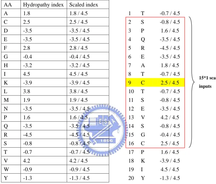
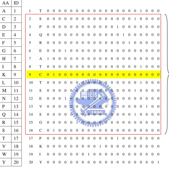
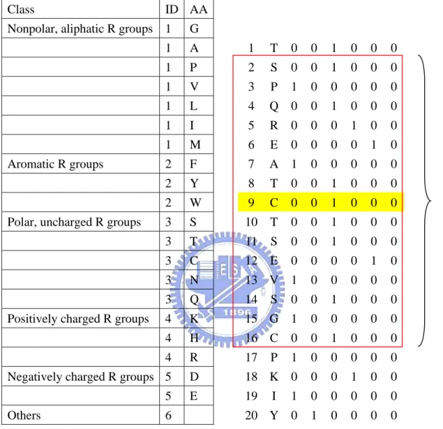
(15) strand and coil.. 2.3.1.3 Hydropathy indexes. In this study, we use the hydropathy indexes to represent each residue (Table 5). In general, the hydropathy indexes can be used to measure the tendency of an amino acid to seek an aqueous environment or a hydrophobic environment. The hydropathy indexes refer to the book “Lehninger Principles of Biochemistry”. Each input vector has 1*15 components (Illustrated in Figure 3). Each. component can be expressed as Hij, where i is the predicted residue and j is the location in the sliding window.. 2.3.1.4 Amino acid in binary coding. We code the protein sequences in binary mode, such as “1 0 0 0 0 0 0 0 0 0 0 0 0 0 0 0 0 0 0 0” represents A (alanine). Each input vector has 20*15 components (Illustrated in Figure 4). Each component can be expressed as AAijk, where i is the predicted residue, j is the location in the sliding window and k is the type of amino acid.. 2.3.1.5 Amino acid properties in binary coding. Knowledge of chemical properties of the standard amino acids is central to an understanding of biochemistry. The chemical properties can be simplified by grouping the standard amino acids into 5 main classes based on the properties of their R groups, and others into the sixth class.(Table 6) The classification refer to the book “Lehninger Principles of Biochemistry”. Each input vector has 6*15 components (Illustrated in Figure 5). Each. component can be expressed as PROPijk, where i is the predicted residue, j is the location in the sliding window and k is the property of amino acid.. -6-.

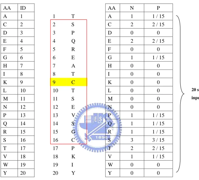
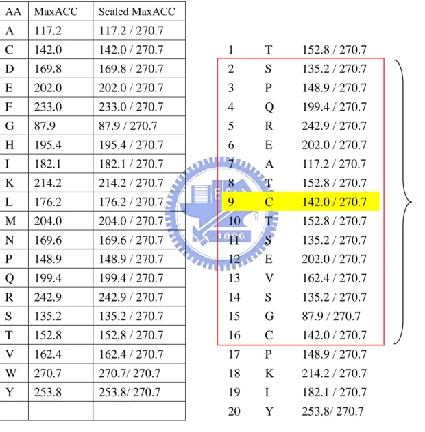
(16) 2.3.1.6 Local amino acid composition. The amino acid percentage is the percentage of each residue in the sliding window. Each input vector has 20 components (Illustrated in Figure 6). Each component can be expressed as LAAik, where i is the predicted residue and k is the type of amino acid.. 2.3.1.7 Local amino acid properties composition. The amino acid properties percentage is the percentage of each residue property in the sliding window. Each input vector has 6 components (Illustrated in Figure 7). Each component can be expressed as LPROPik, where i is the predicted residue, j is the location in the sliding window and k is the property of amino acid.. 2.3.1.8 Residue size. We use the volume of amino acid as the input vector (Table 1). Each input vector has 1*15 components (Illustrated in Figure 8). Each component can be expressed as Rij, where i is the predicted residue and j is the location in the sliding window.. 2.3.2 Global descriptors. We also represent the global environment of sequences by using global sequence composition and global character composition method.. 2.3.2.1 Global amino acid composition -7-.

(17) The amino acid percentage is the percentage of each residue in a given protein sequence totally. Each input vector has 20 components (Illustrated in Figure 9). Each component can be expressed as GAAk, where k is the type of amino acid.. 2.3.2.2 Global amino acid properties composition. The amino acid properties percentage is the percentage of each residue property in a given protein sequence totally. Each input vector has 6 components (Illustrated in Figure 10). Each component can be expressed as GPROPk, where k is the property of amino acid.. 2.4 Performance measures. In order to compare with other works, we use different measures to evaluate 2-state, 3-state and 10-state prediction methods as below.. 2.4.1 In 2-state prediction and 3-state prediction. In this work, two measures are used to evaluate the performance of prediction methods. One is accuracy, the percentage of correctly classified residues, and the other is Matthew’s correlation coefficients (MCC). These measures can be calculated by the following equation:. ∑p Accuracy = c. i. i. (3). N. MCCi =. p i ni − oi u i. ( pi + oi )( pi + ui )(ni + oi )(ni + ui ). (4). Where N is the total number of residues, and c is the class number. And pi, ni, oi and ui are the number of true positives, true negatives, false positives and false negatives for class i, -8-.

(18) respectively. The MCCs have the same value for the two classes in the case of the 2-state prediction.. 2.4.2 In 10-state prediction. Here, we applied several different measures, including the mean absolute error (MAE) of prediction defined as the absolute difference between the predicted and experimental value of relative solvent accessibility, per residue.. MAE =. ∑ ( ASA). pred. − ( ASA)exp. (5). N. Where summation is carried out for all residues and N is the total number of predictions. In addition, Pearson’s “r” is also used in some places, and it is calculated as the ratio of the covariance between the predicted and experimental relative solvent accessibility as below.. r=. N (∑ ( ASA) pred ( ASA)exp ) − (∑ ( ASA) pred )(∑ ( ASA)exp ). [N ∑ (ASA). 2 pred. − (∑ ( ASA) pred ). 2. ][N ∑ (ASA). exp. 2. − (∑ ( ASA)exp ). 2. ]. (6). 2.5 Support vector machine. Support vector machine (SVM), first proposed by Vapnik and co-workers[18] based on statistical learning theory, has quickly become one of the most popular classification and regression methods, due to its flexibility in choosing a similarity function, the ability to handle large feature spaces and accuracy. It has been used in various area, such as protein structure prediction[19], protein fold recognition[20] and microarray data analysis[21].. -9-.

(19) An SVM finds a nonlinear decision function in the input space by implicitly mapping the data into a linear separable higher dimensional feature space and separating the data there by maximizing the geometric margin and minimizing the training error at the same time. Yuan et al.5 implemented SVMlight to predict solvent accessibility. Here, we use LIBSVM version 2.6, which is a multi-class SVM developed by Chang and Lin.[22]. - 10 -.

(20) 3. Server Development and Administration System Overview Figure 2 shows the flowchart of RSA prediction server, and most of the process was built using the Perl language and CGI package. And the prediction result can automatically show on the webpage when the relative solvent accessibility prediction was finished.. - 11 -.

(21) 4. World Wide Web Interface 4.1 Models trained by the three benchmark data sets. User can select an appropriate training dataset of the three benchmark datasets. The consuming time will increase depending on the dataset size.. 4.2 Models of different state thresholds. User can choose a 2-state model (25%), 3-state model (9%;36%) or 10-state model (10%;20%;30%;40%;50%;60%;70%;80%;90%) for different purposes.. 4.3 Query sequence. User can input their query sequence in FASTA format or directly upload the FASTA format file to the SAS prediction server.. 4.4 Website. The RSA prediction server is available at http://e100.life.nctu.edu.tw/~weilun/. Figure3 shows the World Wide Web interface of RSA prediction server. Figure 4 shows the standard output webpage of prediction.. - 12 -.

(22) 5. Results and Discussion 5.1 Prediction accuracies and MCC values using individual local descriptors with RS126 dataset in 2-state prediction model. In the first phase, the performance was evaluated in terms of Qtotal, Qb, Qe and MCC (Table 7). Of the 8 local descriptors, 5 were ranging 65.73% to 75.33%. They are PSSM, amino acid composition, secondary structure profiles, character information and hydropathy indexes in order.. 5.2 Prediction accuracies and MCC values using comprehensive local descriptors with RS126 dataset in 2-state prediction model. In the second phase, we combined the top 5 best-performing local descriptors and 2 global descriptors in many kinds of combinations. In Table 8 we show the results.. Here, we found that PSSM involved more useful information in relative solvent accessibility prediction. The hydropathy indexes performed worse than secondary structure profiles in the individual test, but when combining with PSSM, the hydropathy indexes could increase the prediction accuracy more than the secondary structure profiles did. The combination of these three input vectors can reach the accuracy rate at 77.23% in RS-126 dataset. However, amino acid composition and amino acid properties also seem to offer duplicated information with PSSM, but the amino acid composition could slightly improve the prediction accuracy about 0.5%. The other feature vectors seem not to give useful information about prediction including global descriptors.. - 13 -.

(23) Overall, the best combinations of input vector were PSSM, secondary structure profiles, hydropathy indexes and amino acid composition in this stage. Compared with the individual performance of the 8 different descriptors, the increased accuracy was in the range 68.40% to 77.78%.. 5.3 Prediction accuracies and MCC values of the benchmark test on the RS126, NM215 and KP480 datasets in 2-state prediction model and its comparison with other methods. The performances of prediction in this study are showed in Table9 and Table10. In this stage, the result of top-4 outperforming feature vectors is almost the same as the result of top-3 outperforming feature vectors. To reduce the training space, we took the top-3 outperforming feature vectors as our best work. They are PSSM, secondary structure profiles and hydroparthy indexes. Our best work shows 60.2% accuracy for 3-state prediction (9%;36% thresholds) and 88.4%,81.4%,77.9% and 77.2% for the 2-state prediction with thresholds of 0%,5%,16% and 25% on the RS126 dataset, respectively. It shows slightly better prediction than other methods on the RS126 dataset expect for "Fuzzy k-NN".. 5.4 MAE and Pearson’s “r” values of the benchmark test on the RS126 and KP480 datasets in 10-state prediction model. We used the 10-state prediction model to simulate the real value prediction of solvent accessibility prediction. We took the same measured way to compare with the other real value prediction methods. All results were shown in Table11 and our best work achieved comparable results. The MAE value is 15.2 and Pearson's r is 0.506 in RS-126 dataset. We also transform the 10-state prediction into 2-state to give a rough evaluation. At the threshold of 20%, the accuracy achieved 72.8%, 74.4% in RS-126 and KP-480 dataset.. - 14 -.

(24) 6. Conclusion In this study, our best method achieved the similar performance as the researches did in the recent years. Hence, we can conclude that the three input vectors in our best work can catch enough information to predict relative solvent accessibility accurately.. Our research shows that local descriptors are sufficient for predicting accurately without global descriptors. Secondary structure profiles and hydropathy indexes both can be complementary to PSSM, but in individual case, hydropathy indexes can only achieve poor performance. Sequence information and character information offer overlapped information with PSSM.. In conclusion, our work achieves good prediction accuracy on the three benchmark datasets in 2-state, 3-state and 10-state model. And in the future work, we can apply our method in real value prediction.. - 15 -.

(25) Window of 15 rows. 15*20 scaled inputs. Figure 1. An outline of the PSSM input vectors, which shows how the PSI-BLAST score. matrices are processed.. - 16 -.

(26) Coil. Helix. Strand. 15*3 scaled inputs. Figure 2. The input vectors called “secondary structure profiles”.. - 17 -.

(27) AA. Hydropathy index Scaled index. A. 1.8. 1.8 / 4.5. 1. T. -0.7 / 4.5. C. 2.5. 2.5 / 4.5. 2. S. -0.8 / 4.5. D. -3.5. -3.5 / 4.5. 3. P. 1.6 / 4.5. E. -3.5. -3.5 / 4.5. 4. Q. -3.5 / 4.5. F. 2.8. 2.8 / 4.5. 5. R. -4.5 / 4.5. G. -0.4. -0.4 / 4.5. 6. E. -3.5 / 4.5. H. -3.2. -3.2 / 4.5. 7. A. 1.8 / 4.5. I. 4.5. 4.5 / 4.5. 8. T. -0.7 / 4.5. K. -3.9. -3.9 / 4.5. 9. C. 2.5 / 4.5. L. 3.8. 3.8 / 4.5. 10. T. -0.7 / 4.5. M. 1.9. 1.9 / 4.5. 11. S. -0.8 / 4.5. N. -3.5. -3.5 / 4.5. 12. E. -3.5 / 4.5. P. 1.6. 1.6 / 4.5. 13. V. 4.2 / 4.5. Q. -3.5. -3.5 / 4.5. 14. S. -0.8 / 4.5. R. -4.5. -4.5 / 4.5. 15. G. -0.4 / 4.5. S. -0.8. -0.8 / 4.5. 16. C. 2.5 / 4.5. T. -0.7. -0.7 / 4.5. 17. P. 1.6 / 4.5. V. 4.2. 4.2 / 4.5. 18. K. -3.9 / 4.5. W. -0.9. -0.9 / 4.5. 19. I. 4.5 / 4.5. Y. -1.3. -1.3 / 4.5. 20. Y. -1.3 / 4.5. Figure 3. The input vectors called “hydropathy indexes”.. - 18 -. 15*1 scaled inputs.

(28) AA ID A. 1. 1. T. 0. 0. 0. 0. 0 0. 0. 0. 0. 0. 0. 0. 0. 0. 0. 0. 1. 0. 0. 0. C. 2. 2. S. 0. 0. 0. 0. 0 0. 0. 0. 0. 0. 0. 0. 0. 0. 0. 1. 0. 0. 0. 0. D. 3. 3. P. 0. 0. 0. 0. 0 0. 0. 0. 0. 0. 0. 0. 1. 0. 0. 0. 0. 0. 0. 0. E. 4. 4. Q. 0. 0. 0. 0. 0 0. 0. 0. 0. 0. 0. 0. 0. 1. 0. 0. 0. 0. 0. 0. F. 5. 5. R. 0. 0. 0. 0. 0 0. 0. 0. 0. 0. 0. 0. 0. 0. 1. 0. 0. 0. 0. 0. G. 6. 6. E. 0. 0. 0. 1. 0 0. 0. 0. 0. 0. 0. 0. 0. 0. 0. 0. 0. 0. 0. 0. H. 7. 7. A. 1. 0. 0. 0. 0 0. 0. 0. 0. 0. 0. 0. 0. 0. 0. 0. 0. 0. 0. 0. I. 8. 8. T. 0. 0. 0. 0. 0 0. 0. 0. 0. 0. 0. 0. 0. 0. 0. 0. 1. 0. 0. 0. K. 9. 9. C. 0. 1. 0. 0. 0 0. 0. 0. 0. 0. 0. 0. 0. 0. 0. 0. 0. 0. 0. 0. L. 10. 10. T. 0. 0. 0. 0. 0 0. 0. 0. 0. 0. 0. 0. 0. 0. 0. 0. 1. 0. 0. 0. M. 11. 11. S. 0. 0. 0. 0. 0 0. 0. 0. 0. 0. 0. 0. 0. 0. 0. 1. 0. 0. 0. 0. N. 12. 12. E. 0. 0. 0. 1. 0 0. 0. 0. 0. 0. 0. 0. 0. 0. 0. 0. 0. 0. 0. 0. P. 13. 13. V. 0. 0. 0. 0. 0 0. 0. 0. 0. 0. 0. 0. 0. 0. 0. 0. 0. 1. 0. 0. Q. 14. 14. S. 0. 0. 0. 0. 0 0. 0. 0. 0. 0. 0. 0. 0. 0. 0. 1. 0. 0. 0. 0. R. 15. 15. G. 0. 0. 0. 0. 0 1. 0. 0. 0. 0. 0. 0. 0. 0. 0. 0. 0. 0. 0. 0. S. 16. 16. C. 0. 1. 0. 0. 0 0. 0. 0. 0. 0. 0. 0. 0. 0. 0. 0. 0. 0. 0. 0. T. 17. 17. P. 0. 0. 0. 0. 0 0. 0. 0. 0. 0. 0. 0. 1. 0. 0. 0. 0. 0. 0. 0. V. 18. 18. K. 0. 0. 0. 0. 0 0. 0. 0. 0. 1. 0. 0. 0. 0. 0. 0. 0. 0. 0. 0. W. 19. 19. I. 0. 0. 0. 0. 0 0. 0. 1. 0. 0. 0. 0. 0. 0. 0. 0. 0. 0. 0. 0. Y. 20. 20. Y. 0. 0. 0. 0. 0 0. 0. 0. 0. 0. 0. 0. 0. 0. 0. 0. 0. 0. 0. 1. Figure 4. The input vectors called “amino acid in binary coding”.. - 19 -. 15*20 scaled inputs.

(29) Class. ID AA. Nonpolar, aliphatic R groups 1. G. 1. A. 1. T. 0. 0. 1. 0. 0. 0. 1. P. 2. S. 0. 0. 1. 0. 0. 0. 1. V. 3. P. 1. 0. 0. 0. 0. 0. 1. L. 4. Q 0. 0. 1. 0. 0. 0. 1. I. 5. R. 0. 0. 0. 1. 0. 0. 1. M. 6. E. 0. 0. 0. 0. 1. 0. 2. F. 7. A 1. 0. 0. 0. 0. 0. 2. Y. 8. T. 0. 0. 1. 0. 0. 0. 2. W. 9. C. 0. 0. 1. 0. 0. 0. 3. S. 10. T. 0. 0. 1. 0. 0. 0. 3. T. 11. S. 0. 0. 1. 0. 0. 0. 3. C. 12. E. 0. 0. 0. 0. 1. 0. 3. N. 13 V 1. 0. 0. 0. 0. 0. 3. Q. 14. 0. 0. 1. 0. 0. 0. 4. K. 15 G 1. 0. 0. 0. 0. 0. 4. H. 16 C. 0. 0. 1. 0. 0. 0. 4. R. 17. 1. 0. 0. 0. 0. 0. Negatively charged R groups 5. D. 18 K 0. 0. 0. 1. 0. 0. 5. E. 19. 1. 0. 0. 0. 0. 0. 20 Y 0. 1. 0. 0. 0. 0. Aromatic R groups. Polar, uncharged R groups. Positively charged R groups. Others. 6. S. P I. Figure 5. The input vectors called “amino acid properties in binary coding”.. - 20 -. 15*6 scaled inputs.

(30) AA. ID. A. 1. 1. C. 2. D. AA. N. P. T. A. 1. 1 / 15. 2. S. C. 2. 2 / 15. 3. 3. P. D. 0. 0. E. 4. 4. Q. E. 2. 2 / 15. F. 5. 5. R. F. 0. 0. G. 6. 6. E. G. 1. 1 / 15. H. 7. 7. A. H. 0. 0. I. 8. 8. T. I. 0. 0. K. 9. 9. C. K. 0. 0. L. 10. 10. T. L. 0. 0. 20 scaled. M. 11. 11. S. M. 0. 0. inputs. N. 12. 12. E. N. 0. 0. P. 13. 13. V. P. 1. 1 / 15. Q. 14. 14. S. Q. 1. 1 / 15. R. 15. 15. G. R. 1. 1 / 15. S. 16. 16. C. S. 3. 3 / 15. T. 17. 17. P. T. 2. 2 / 15. V. 18. 18. K. V. 1. 1 / 15. W. 19. 19. I. W. 0. 0. Y. 20. 20. Y. Y. 0. 0. Figure 6. The input vectors called “local amino acid composition”.. - 21 -.

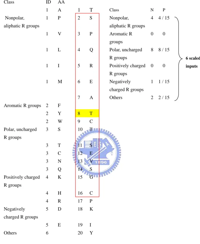
(31) Class Nonpolar,. ID. AA. 1. A. 1. T. Class. N. P. 1. P. 2. S. Nonpolar,. 4. 4 / 15. 0. 0. 8. 8 / 15. aliphatic R groups. aliphatic R groups 1. V. 3. P. Aromatic R groups. 1. L. 4. Q. Polar, uncharged R groups. 1. I. 5. R. Positively charged. 6 scaled. 0. 0. 1. 1 / 15. 2. 2 / 15. R groups 1. M. 6. E. Negatively charged R groups. Aromatic R groups. Polar, uncharged. 7. A. 2. F. 2. Y. 8. T. 2. W. 9. C. 3. S. 10. T. 3. T. 11. S. 3. C. 12. E. 3. N. 13. V. 3. Q. 14. S. 4. K. 15. G. 4. H. 16. C. 4. R. 17. P. 5. D. 18. K. 5. E. 19. I. 20. Y. Others. R groups. Positively charged R groups. Negatively charged R groups Others. 6. Figure 7. The input vectors called “local amino acid properties composition”.. - 22 -. inputs.

(32) AA. MaxACC. Scaled MaxACC. A. 117.2. 117.2 / 270.7. C. 142.0. 142.0 / 270.7. 1. T. 152.8 / 270.7. D. 169.8. 169.8 / 270.7. 2. S. 135.2 / 270.7. E. 202.0. 202.0 / 270.7. 3. P. 148.9 / 270.7. F. 233.0. 233.0 / 270.7. 4. Q. 199.4 / 270.7. G. 87.9. 87.9 / 270.7. 5. R. 242.9 / 270.7. H. 195.4. 195.4 / 270.7. 6. E. 202.0 / 270.7. I. 182.1. 182.1 / 270.7. 7. A. 117.2 / 270.7. K. 214.2. 214.2 / 270.7. 8. T. 152.8 / 270.7. L. 176.2. 176.2 / 270.7. 9. C. 142.0 / 270.7. M. 204.0. 204.0 / 270.7. 10. T. 152.8 / 270.7. N. 169.6. 169.6 / 270.7. 11. S. 135.2 / 270.7. P. 148.9. 148.9 / 270.7. 12. E. 202.0 / 270.7. Q. 199.4. 199.4 / 270.7. 13. V. 162.4 / 270.7. R. 242.9. 242.9 / 270.7. 14. S. 135.2 / 270.7. S. 135.2. 135.2 / 270.7. 15. G. 87.9 / 270.7. T. 152.8. 152.8 / 270.7. 16. C. 142.0 / 270.7. V. 162.4. 162.4 / 270.7. 17. P. 148.9 / 270.7. W. 270.7. 270.7/ 270.7. 18. K. 214.2 / 270.7. Y. 253.8. 253.8/ 270.7. 19. I. 182.1 / 270.7. 20. Y. 253.8/ 270.7. Figure 8. The input vectors called “residue size”.. - 23 -. 15 scaled inputs.

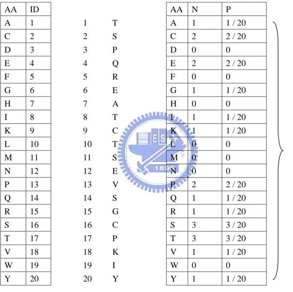
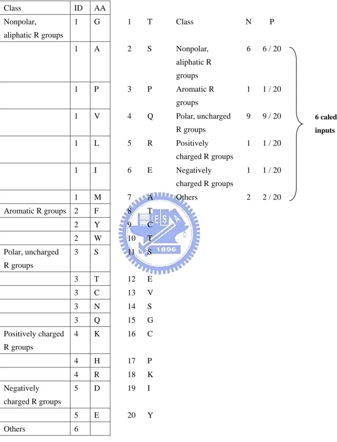
(33) AA. N. P. T. A. 1. 1 / 20. 2. S. C. 2. 2 / 20. 3. 3. P. D. 0. 0. E. 4. 4. Q. E. 2. 2 / 20. F. 5. 5. R. F. 0. 0. G. 6. 6. E. G. 1. 1 / 20. H. 7. 7. A. H. 0. 0. I. 8. 8. T. I. 1. 1 / 20. K. 9. 9. C. K. 1. 1 / 20. L. 10. 10. T. L. 0. 0. M. 11. 11. S. M. 0. 0. N. 12. 12. E. N. 0. 0. P. 13. 13. V. P. 2. 2 / 20. Q. 14. 14. S. Q. 1. 1 / 20. R. 15. 15. G. R. 1. 1 / 20. S. 16. 16. C. S. 3. 3 / 20. T. 17. 17. P. T. 3. 3 / 20. V. 18. 18. K. V. 1. 1 / 20. W. 19. 19. I. W. 0. 0. Y. 20. 20. Y. Y. 1. 1 / 20. AA. ID. A. 1. 1. C. 2. D. Figure 9. The input vectors called “global amino acid composition”.. - 24 -. 20 scaled inputs.

(34) Class. ID. AA. Nonpolar,. 1. G. 1. T. Class. N. P. 1. A. 2. S. Nonpolar,. 6. 6 / 20. 1. 1 / 20. 9. 9 / 20. aliphatic R groups aliphatic R groups 1. P. 3. P. Aromatic R groups. 1. V. 4. Q. Polar, uncharged R groups. 1. L. 5. R. Positively. inputs. 1. 1 / 20. 1. 1 / 20. 2. 2 / 20. charged R groups 1. I. 6. E. Negatively charged R groups. Aromatic R groups. Polar, uncharged. 1. M. 7. A. 2. F. 8. T. 2. Y. 9. C. 2. W. 10. T. 3. S. 11. S. 3. T. 12. E. 3. C. 13. V. 3. N. 14. S. 3. Q. 15. G. 4. K. 16. C. 4. H. 17. P. 4. R. 18. K. 5. D. 19. I. 5. E. 20. Y. Others. R groups. Positively charged R groups. Negatively charged R groups Others. 6. Figure 10. The input vectors called “global amino acid properties composition”.. - 25 -. 6 caled.

(35) Query Sequence. PSI-BLAST. PSSM. PSIPRED. SS Profiles. Hydropathy Indexes. Standard SVM File. SVM Model. SVM-PREDICT. SVM Output File. Figure 11. The figure shows the components of SAS prediction server, and most of the. connection was built using the Perl language and CGI package.. - 26 -.

(36) Figure 12. The World Wide Web interface of the RSA prediction server.. - 27 -.

(37) *Prob X: probability of the residue belongs to class X *PredRSA: the predicted relative class. Figure 13. The standard output webpage of prediction.. - 28 -.

(38) Tables. Table 1. Maximum value of solvent accessible surface areas of each kind of residue calculated by MOLSIM program. Amino acid. MaxACC. A. 117.2. B C D E F G H I K L M N P Q R S T V W X Y Z. 160.0 142.0 169.8 202.0 233.0 87.9 195.4 182.1 214.2 176.2 204.0 169.6 148.9 199.4 242.9 135.2 152.8 162.4 270.7 180.0 253.8 196.0. - 29 -.

(39) Table 2. The RS126 dataset used in this study. 256b_a 9api_b 7cat_a 6cpa_ 3ebx_ 2fox_ 6hir_ 1l58_ 2mev_4 1pyp_ 3rnt_ 2stv_ 2utg_a 2aat_ 1azu_ 1cbh_ 6cpp_ 5er2_e 1g6n_a 3hmg_a 1lap_ 2or1_l 1r09_2 7rsa_ 2tgp_i 9wga_a. 8abp_ 1cyo_ 1cc5_ 4cpv_ 1etu_ 2gbp_ 3hmg_b 5ldh_ 1ovo_a 2mhu_ 2rsp_a 1tgs_i 2wrp_r 6acn_ 1bbp_a 2ccy_a 1crn_ 1fc2_c 1a45_ 2hmz_a 1gdj_ 2pab_a 1mrt_ 4rxn_ 3tim_a 1bks_a. 1acx_ 1bds_ 1cdh_ 1cse_i 1fdl_h 1gdl_o 5hvp_a 2lhb_ 1paz_ 1ppt_ 1s01_ 6tmn_e 1bks_b 8adh_ 1bmv_1 1cdt_a 6cts_ 1dur_ 2gls_a 2i1b_ 1lmb_3 9pap_ 1rbp_ 3sdh_a 2tmv_p 4xia_a. - 30 -. 3ait_ 1bmv_2 3cla_ 2cyp_ 1fkf_ 2gn5_ 3icb_ 2ltn_a 2pcy_ 1rhd_ 4sgb_i 1tnf_a 1prc_c 2ak3_a 3blm_ 3cln_ 5cyt_r 1fnd_ 1gp1_a 7icd_ 2ltn_b 4pfk_ 4rhv_1 1sh1_ 4ts1_a 1prc_h. 2alp_ 4bp2_ 4cms_ 1eca_ 1iqz_ 4gr1_ 1il8_a 5lyz_ 3pgm_ 4rhv_3 2sns_ 2tsc_a 1prc_l 9api_a 2cab_ 4cpa_i 6dfr_ 1fxi_a 1hip_ 9ins_b 1mcp_l 2phh_ 4rhv_4 2sod_b 1ubq_ 1prc_m.

(40) Table 3. The NM215 dataset used in this study. 119l_ 1bnca 1dktb 1ggga 1knya 1ofga 1pud_ 1svpa 1vls_ 2chsa 2sns_ 153l_ 1btma 1dkza 1gnd_ 1kpta 1onra 1pyta 1tadc 1wba_ 2ctc_ 2tysa 1aba_ 1btn_ 1dosa 1gotb 1kte_ 1opr_ 1qapa 2tdx_ 1whi_. 2end_ 3chy_ 1abrb 1cem_ 1dxy_ 1gpc_ 1kuh_ 1ospo 1ra9_ 1tfe_ 1who_ 2gdm_ 3cox_ 1afra 1ceo_ 1ecea 1gpl_ 1lba_ 1pbc_ 1rcf_ 1tfr_ 1bksb 2hft_ 3grs_ 1afwa 1cewi 1ecpa 1gsa_ 1lcl_ 1pda_ 1rec_. 1thv_ 1xgsa 2hhma 3mdda 1amm_ 1cfya 1ede_ 1gtma 1lki_ 1pdo_ 1rgs_ 1thx_ 1xnb_ 2hpda 3minb 1amp_ 1chd_ 1edg_ 1hava 1lkka 1pea_ 1rnl_ 1tib_ 1xvaa 2i1b_ 3nll_ 1aoca 1chka 1edt_ 1hfc_ 1ltsa. 1pex_ 1rro_ 1tml_ 1xyza 2liv_ 3sdha 1atla 1chma 1erv_ 1hgxa 1mai_ 1pgs_ 1rsy_ 1tupc 1yasa 2mtac 5p21_ 1atna 1cmke 1esc_ 1hlb_ 1maz_ 1phe_ 1rvaa 1tys_ 1ysc_ 2naca 5ptp_ 1axn_ 1cnv_ 1exnb. - 31 -. 1hsba 1mbd_ 1php_ 1sbp_ 1ubi_ 1ytw_ 2pgd_ 6gsva 1bbpa 1csee 1ezm_ 1htp_ 1mkaa 1pioa 1sftb 1uby_ 256ba 2phla 6pfka 1bdo_ 1csga 1fds_ 1idaa 1mlda 1plc_ 1sig_ 1udii 2abk_ 2phy_ 7rsa_ 1beo_. 1csn_ 1fjma 1ido_ 1mml_ 1pmi_ 1slua 1uxy_ 2arca 2pia_ 8atcb 1bfg_ 1cyx_ 1ftpa 1ifc_ 1mola 1pne_ 1smea 1vcaa 2ayh_ 2pspa 1bgc_ 1deaa 1fua_ 1irk_ 1nar_ 1poa_ 1smpi 1vhh_ 2bbvc 2rn2_ 1bhmb. 1dela 1gai_ 1itg_ 1nbab 1poc_ 1sra_ 1vhra 1m85_ 2rspb 1bib_ 1dfji 1gcb_ 1jkw_ 1nox_ 1pot_ 1std_ 1vid_ 2cba_ 2scpa 1bmfg 1dhr_ 1gdoa 1knb_ 1noza 1ppn_ 1stfi 1vin_ 2ccya 2sil_.

(41) Table 4. The KP480 dataset used in this study. 154l-1-AUTO.1. 1cbg-1-AS. 1ctn-1-AS.1. 1edd-1-DOMAK. 2gep-3-AS. 1aazb-1-DOMAK. 1cbh. 1ctn-3-AS.1. 1edmc-1-AUTO.1. 1gflb-1-AS. 1acx. 1cc5. 1ctu-1-AUTO.1. 1eft-3-DOMAK. 1ghsb-1-GJB. 1add-1-AS. 1cdta. 1ctu-2-AUTO.1. 1efud-2-AUTO.1. 1gky-2-AS. 1adeb-2-AUTO.1. 1cei-1-GJB. 1eu1a-4-AUTO.1. 1epbb-1-DOMAK. 1gln-2-AS. 1ahb-2-GJB. 1celb-1-AUTO.1. 1cyx-1-AUTO.1. 1ese-1-AUTO.1. 1gln-4-AS. 1alkb-1-AS. 1cem-1-GJB. 1daab-1-AS. 1esl-1-GJB. 1gmpb-1-DOMAK. 1amp-1-AS. 1cewi-1-DOMAK. 1daab-2-AS. 1etu. 1gnd-2-JAC. 1aorb-1-AS. 1cfb-1-AS. 1dar-3-AS. 1euu-2-JAC. 1gog-1-AS.1. 1aorb-3-AS. 1cgu-2-GJB. 1dfji-1-AUTO.1. 1fbab-1-DOMAK. 1gog-2-AS.1. 1aozb-1-AS. 1cgu-3-GJB. 1dih-2-AS. 1fbl-1-AS. 1gog-3-AS.1. 1aozb-2-AS. 1cgu-4-GJB. 1dik-1-AS.1. 1fc2c. 1gp1a. 1aozb-3-AS. 2chbe-1-DOMAK. 1dik-2-AS.1. 1fdlh. 1gp2g-2-AS. 1asw-1-AUTO.1. 1chd-1-AS. 1dik-3-AS.1. 1fdt-1-AS. 1gpc-1-AS. 1avhb-3-AS. 1chkb-2-AUTO.1. 1dik-4-AS.1. 1dur. 1gpmd-4-AS. 1avhb-4-AS. 1chmb-1-DOMAK. 1din-1-AS. 1find-1-AUTO.1. 1gpmd-5-AS. 1ayab-1-GJB. 1cksc-1-AUTO.1. 1dkza-1-JAC. 1find-2-AUTO.1. 1grj-1-AS. 1azu. 1clc-1-AS.1. 1dlc-1-AS.1. 1fjmb-2-AS. 1grj-2-AS. 1bam-1-AS. 1clc-2-AS.1. 1dlc-3-AS.1. 1fkf. 1gtmc-2-AUTO.1. 1bbpa. 1clc-3-AS.1. 1dnpb-1-AUTO.1. 1fnd. 1gtqb-1-AUTO.1. 1bcx-1-DOMAK. 1cnsb-1-AUTO.1. 1dnpb-2-AUTO.1. 1fua-1-AUTO.1. 1gym-1-AUTO.1. 1bdo-1-AS. 1colb-1-DOMAK. 1dpgb-1-AUTO.1. 1fuqb-1-AUTO.1. 1han-1-AUTO.1. 1bet-1-DOMAK. 1comc-1-DOMAK. 1dpgb-2-AUTO.1. 1fuqb-2-AUTO.1. 1han-2-AUTO.1. 1bfg-1-DOMAK. 1cpcl-1-DOMAK. 1dsbb-2-AUTO.1. 1fuqb-3-AUTO.1. 1hcgb-1-AS. 1bmv1. 1cpn-1-DOMAK. 1dts-1-AUTO.1. 1fxia. 1hcra-1-DOMAK. 1bmv2. 1cqa-1-AUTO.1. 1dupa-1-AS. 1gal-2-AS. 1hip. 1bncb-1-AS. 1crn. 1dynb-1-AUTO.1. 1gal-3-AS. 1hiws-1-AS. 1bncb-3-AS. 1csei. 1eca. 1gcb-2-AS. 1hjrd-1-AUTO.1. 1bncb-4-AS. 1csmb-1-AUTO.1. 1eceb-1-AUTO.1. 1gcmc-1-AUTO.1. 1hmpb-1-AUTO.1. 1bovb-1-DOMAK. 1ctf-1-DOMAK. 1ecl-1-AS. 1gd1o. 1hnf-1-AS. 1brse-1-DOMAK. 2cthb-1-DOMAK. 1ecl-4-AS. 1gdj. 1hnf-2-AS. 1bsdb-1-DOMAK. 1ctm-2-DOMAK. 1ecpf-1-AUTO.1. 2gep-2-AS. 1horb-1-AUTO.1. - 32 -.

(42) Table 4. The KP480 dataset used in this study (continued). 1hplb-1-AS. 1lehb-3-AS. 1nozb-2-AUTO.1. 1ptr-1-AUTO.1. 1sfe-1-AS. 1hplb-2-AS. 1lib-1-DOMAK. 1oacb-1-AS.1. 1ptx-1-AS. 1sfe-2-AS. 1hslb-2-DOMAK. 1lis-1-DOMAK. 1oacb-2-AS.1. 1pyp. 1sftb-2-AS. 1htrp-1-AS. 1lki-1-AS. 1oacb-3-AS.1. 1pyta-1-AS. 1sh1. 1hvq-1-AUTO.1. 1lmb3. 1oacb-4-AS.1. 1qbb-1-AUTO.1. 1smnb-1-AUTO.1. 1hxn-1-AS. 1lpba-1-DOMAK. 1onrb-1-AUTO.1. 1qbb-2-AUTO.1. 1smpi-1-AS. 1hyp-1-DOMAK. 1lpe-1-DOMAK. 1otgc-1-AS. 1qbb-3-AUTO.1. 1spbp-1-AS. 1ignb-2-GJB. 1mai-1-JAC. 1ovb-1-GJB. 1qbb-4-AUTO.1. 1sra-1-AS. 1il8a. 1masb-1-AUTO.1. 1ovoa. 1qrdb-1-AUTO.1. 1srja-1-DOMAK. 1ilk-1-AS. 1mdam-1-DOMAK. 1oxy-3-AS. 1r092. 1stfi-1-DOMAK. 1ilk-2-AS. 1mdta-1-AS. 1oyc-1-AS. 1rbp. 1stme-1-AUTO.1. 1inp-1-AS.1. 1mdta-2-AS. 1paz. 1rec-1-DOMAK. 1svb-1-AS. 1inp-2-AS.1. 1mdta-3-AS. 1pbp-2-DOMAK. 1rec-2-DOMAK. 1svb-2-AS. 1irk-1-AS. 1mjc-1-DOMAK. 1pbwb-1-AS. 1regy-1-AUTO.1. 1tabi-1-DOMAK. 1irk-2-AS. 1mla-2-AS.1. 1pda-2-AS. 1reqc-2-AS. 1taq-2-AS. 1isab-1-GJB. 1mmoh-1-AS. 1pda-3-AS. 1rhd. 1tcra-2-GJB. 1isab-2-GJB. 1mns-2-AS. 1pdnc-2-AS. 1rhgc-1-DOMAK. 1tfr-1-GJB. 1isub-1-DOMAK. 1mof-1-AS. 1pdo-1-GJB. 1rie-1-GJB. 1thtb-1-AUTO.1. 1jud-1-GJB. 1mrrb-1-DOMAK. 1pga-1-DOMAK. 1ris-1-DOMAK. 1thx-1-AUTO.1. 1kimb-1-AUTO.1. 1mrt. 1pht-1-AUTO.1. 1rlds-1-DOMAK. 1tie-1-DOMAK. 1knb-1-AS. 1mspb-1-AS. 1pii-2-DOMAK. 1rlr-1-JAC. 1tif-1-AS. 1krca-1-AUTO.1. 1nal4-1-AUTO.1. 1pkyc-2-AUTO.1. 1rlr-2-JAC. 1tig-1-AUTO.1. 1krcb-1-AS. 1nar-1-DOMAK. 1pkyc-3-AUTO.1. 1rpo-1-AUTO.1. 1tml-1-AS. 1kte-1-AS. 1nbac-1-AS. 1pmi-2-GJB. 1rsy-1-AS. 1tndb-2-DOMAK. 1ktq-1-AUTO.1. 1ncg-1-AUTO.2. 1pnmb-2-AS. 1rvvz-1-AUTO.1. 1tnfa. 1kuh-1-AS. 1ndh-1-AS. 1pnt-1-AS. 1s01. 1tplb-3-AS. 1l58. 1ndh-2-AS. 1poc-1-DOMAK. 1scud-1-AS. 1trb-2-AS. 1lap. 1nfp-1-AS. 1powb-1-DOMAK. 1scue-2-AS. 1trh-1-AS. 1latb-1-AUTO.1. 1nga-2-AS.1. 1powb-2-DOMAK. 1scue-3-AS. 1trkb-1-AS. 1lba-1-DOMAK. 1nlkl-1-DOMAK. 1powb-3-DOMAK. 1seib-1-AUTO.1. 1trkb-3-AS. 1lbu-1-AS. 1nol-1-AUTO.2. 1ppi-2-AS. 1seib-2-AUTO.1. 1tsp-1-AS. 1lbu-2-AS. 1nox-1-GJB. 1ppt. 1sesa-2-AS. 2tssb-2-DOMAK. - 33 -.

(43) Table 4. The KP480 dataset used in this study (continued). 1tul-1-JAC. 2afnc-2-AUTO.1. 2i1b. 2utga. 4fisb-1-DOMAK. 1tupc-1-AUTO.1. 2ak3a. 2ltna. 2wrpr. 4gr1. 1ubq. 2alp. 2ltnb. 2yhx-3-DOMAK. 4pfk. 1udh-1-AUTO.1. 2asr-1-DOMAK. 2mev4. 3ait. 4rhv1. 1umub-1-AS. 2bat-1-GJB. 2mtac-1-AS. 1cyo. 4rhv3. 1vcab-1-AUTO.1. 2bltb-2-AUTO.1. 2nadb-2-AS.1. 4bcl-1-DOMAK. 4rhv4. 1vcab-2-AUTO.1. 2bopa-1-DOMAK. 2npx-3-AS.1. 3blm. 4rxn. 1vcc-1-AS. 2cab. 2olba-2-AS. 3cd4. 4sdha. 1vhh-1-AS. 2ccya. 2olba-3-AS. 3chy-1-DOMAK. 4sgbi. 1vhrb-2-AUTO.1. 2cmd-2-GJB. 2or1l. 3cla. 4ts1a. 1vid-1-JAC. 2cpo-1-AUTO.1. 2paba. 3cln. 4xiaa. 1vjs-3-GJB. 2cyp. 2pgd-1-AUTO.1. 3cox-1-AS.1. 5cytr. 1vmob-1-AS. 2dkb-2-AS. 2pgd-2-AUTO.1. 3cox-2-AS.1. 5er2e. 1vnc-1-JAC. 2dln-1-AS. 2phh. 3ecab-1-AS. 5ldh. 1vokb-1-AS. 2dln-3-AS. 2phy-1-GJB. 3ecab-2-AS. 5lyz. 1vpt-1-JAC. 2dnja-1-AS. 2polb-1-AS. 1g6na. 5sici-1-DOMAK. 1wapv-1-AUTO.1. 2ebn-1-AS. 2reb-1-DOMAK. 3hmga. 6acn. 1whi-1-AS. 2end-1-DOMAK. 2reb-2-DOMAK. 3hmgb. 6cpa. 1bksa. 2fox. 2rsla-1-GJB. 3icb. 6cpp. 1bksb. 1iqz. 2rspa. 3inkd-1-DOMAK. 6cts. 1xvab-1-GJB. 2gbp. 2scpb-1-DOMAK. 3mddb-1-AS. 6dfr. 1yptb-1-AUTO.1. 1a45. 2sil-1-AS. 3mddb-2-AS. 6hir. 1yrna-2-AS. 2glsa. 2sns. 3mddb-3-AS. 6tmne. 1znbb-1-AS. 2gn5. 2sodb. 3pgk-2-AS. 7cata. 1zymb-2-AUTO.1. 2gsq-2-AS. 2spt-1-DOMAK. 3pgm. 7icd. 256ba. 2hft-1-AS. 2spt-2-DOMAK. 3pmgb-1-AS. 7rsa. 2aaib-2-DOMAK. 2hft-2-AS. 2tgi-1-DOMAK. 3pmgb-2-AS. 821p-1-DOMAK. 2aat. 2hhmb-1-DOMAK. 2tgpi. 3pmgb-3-AS. 8adh. 2abk-2-AS. 2hhmb-2-DOMAK. 2tmdb-3-AS. 3pmgb-4-AS. 9apia. 2admb-1-AUTO.1. 2hipb-1-DOMAK. 2tmvp. 3rnt. 9apib. 2admb-2-AUTO.1. 2hmza. 2trt-1-AUTO.1. 3tima. 9pap. 2afnc-1-AUTO.1. 2hpr-1-DOMAK. 2tsca. 4bp2. 9wgaa. - 34 -.

(44) Table 5. The hydropathy index of the standard amino acids.. Amino acid. Hydropathy index. A C D E F G H I K L M N P Q R S T V W Y. 1.8 2.5 -3.5 -3.5 2.8 -0.4 -3.2 4.5 -3.9 3.8 1.9 -3.5 1.6 -3.5 -4.5 -0.8 -0.7 4.2 -0.9 -1.3. - 35 -.

(45) Table 6. The classification of the standard amino acids by R groups.. Class. Amino acid. Nonpolar, aliphatic R groups. G A P V L I M F Y W S T C N Q K H R D E. Aromatic R groups. Polar, uncharged R groups. Positively charged R groups. Negatively charged R groups. - 36 -.

(46) Table 7. Prediction accuracies and MCC values using individual local descriptors with RS126 datasets in 2-state prediction model.. Features. Threshold. Qtotal. Qb. Qe. MCC. PSSM. 25. 75.33. 76.38. 74.11. 50.43. Hydropathy indexes. 25. 65.73. 80.43. 48.61. 30.79. Secondary structure profile. 25. 67.80. 68.93. 66.46. 35.34. Amino acid in binary coding. 25. 70.59. 74.49. 66.06. 40.70. Amino acid properties in binary coding. 25. 67.34. 69.51. 64.81. 34.31. Local amino acid composition. 25. 58.22. 72.67. 41.39. 14.82. Local amino acid properties composition. 25. 58.04. 75.85. 37.30. 14.27. Residue size. 25. 55.8. 96.19. 8.68. 10.18. - 37 -.

(47) Table 8. Prediction accuracies and MCC values using comprehensive local descriptors with RS126 datasets in 2-state prediction model.. Features. Threshold. Qtotal. Qb. Qe. MCC. PSSM+H. 25. 76.45. 78.96. 73.52. 52.57. PSSM+SS. 25. 75.98. 79.06. 72.40. 51.60. H+SS. 25. 68.40. 70.05. 66.48. 36.50. PSSM+H+SS. 25. 77.23. 78.53. 75.72. 54.23. PSSM+H+SS+AA. 25. 77.78. 79.44. 75.84. 55.29. PSSM+H+SS+PROP. 25. 77.40. 79.15. 75.36. 54.53. PSSM+H+SS+AA+PROP. 25. 77.33. 78.64. 75.80. 54.42. PSSM+H+SS+GAA. 25. 77.28. 78.48. 75.88. 54.33. PSSM+H+SS+GPROP. 25. 77.15. 78.29. 75.82. 54.07. *H: hydropathy indexes *SS: secondary structure profile *AA: amino acid in binary coding *PROP: amino acid properties in binary coding *GAA: Global amino acid composition *GPROP: Global amino acid properties composition. - 38 -.

(48) Table 9. Prediction accuracies of the benchmark tests on the RS126, NM215 and KP480 datasets in 2-state prediction model and its comparison with other methods. Year. Method. State threshold 25%. 20%. 16%. 5%. 0%. 9,36%. -. -. 74.8. -. 86.0. 57.5. 1994. PHDacc(RS126)[3]. 2000. Jnet(CB480)[7]. 76.2. -. -. 79.8. 86.5. -. 2002. BRNNs (PDB-1086)[4]. 77.2. 77.5. -. 81.2. 86.5. -. 2003. PP(RS-126)[23]. -. -. 75.1. -. -. 57.9. 2003. NETASA(NM-215)[24]. 70.3. -. -. 74.6. 87.9. -. 2004. SVMpsi (RS126)[13]. 76.8. -. 77.8. 79.8. 86.2. 59.6. 2004. SVMpsi(KP480)[13]. 78.7. -. 80.7. 82.4. 87.4. 64.5. 2005. Fuzzy k-NN(RS-126)[14]. 78.3. -. 79.0. 82.2. 87.2. 63.8. 2005. SVR12(RA-603)[10]. 76.7. 76.8. -. 76.5. -. -. 2005. WE(2148 chains)[1]. -. 80.0. -. -. -. -. PSSM+H+SS (RS126). 77.2. 77.6. 77.9. 81.4. 88.4. 60.2. PSSM+H+SS+AA (RS126). 77.8. 77.8. 78.1. 80.0. 88.8. 61.6. PSSM+H+SS (NM215). 78.3. 77.7. 87.2. 87.4. 87.0. 62.7. PSSM+H+SS (KP480). 78.0. 78.5. 81.3. 87.0. 62.3. - 39 -.

(49) Table 10. MCC values of the benchmark tests on the RS126, NM215 and KP480 datasets in 2-state prediction model and its comparison with other methods. Year. Method. State threshold 25%. 20%. 16%. 5%. 0%. 9,36%. 1994. PHDacc(RS126)[3]. -. -. -. -. -. -. 2000. Jnet(CB480)[7]. -. -. -. -. -. -. 2002. BRNNs (PDB-1086)[4]. -. -. -. -. -. -. 2003. PP(RS-126)[23]. -. -. 48.5. -. -. 53.0. 2003. NETASA(NM-215)[24]. -. -. -. -. -. -. 2004. SVMpsi (RS126)[13]. -. -. -. -. -. -. 2004. SVMpsi(KP480)[13]. -. -. -. -. -. -. 2005. Fuzzy k-NN(SCOP-229)[14]. 55.4. -. 56.0. 54.1. 43.1. 56.0;19.9;50.8. 2005. SVR12(RA-603)[10]. -. -. -. -. -. -. 2005. WE(2148 chains)[1]. -. 60.0. -. -. -. -. PSSM+H+SS (RS126). 54.2. 55.2. 54.7. 49.7. 22.2. 52.0;17.0;48.4. PSSM+H+SS+AA (RS126). 55.3. 55.6. 55.2. 45.7. 31.7. 53.2;19.3;50.8. PSSM+H+SS (NM215). 56.0. 56.5. 34.2. 36.4. 38.3. 56.3;20.9;50.7. PSSM+H+SS (KP480). 55.1. 56.6. 53.2. 35.8. 55.2;19.9;50.9. - 40 -.

(50) Table 11. MAE and Pearson’s “r” values of the benchmark tests on the RS126 and KP480 datasets in 10-state prediction model. Data Set. MAE. R. Accuracy. RS-126. 19.4. 0.477. 71%(16%). Carugo-338. 19.0. 0.490. CB-502. 18.8. 0.482. CB-502. 18.5. 0.520. YH-1277. 17.0. 0.617. 74.6%(15%). SABLE[5]. RA-603. 15.3-15.8. 0.64-0.67. 77%(15%). SVR1218. RA-603. 15.8-16.6. 0.62-0.63. 75.8(15%). PSSM+H+SS. RS-126. 15.2. 0.506. 72.8(20%). KP-480. 14.1. 0.537. 74.4(20%). Year 2003. 2004. 2005. Method RVP16 P. SVR[25]. - 41 -.

(51) 參考文獻 1.. Chen, H. and H.X. Zhou, Prediction of solvent accessibility and sites of deleterious. 3.. mutations from protein sequence. Nucleic Acids Res, 2005. 33(10): p. 3193-9. Wang, Z. and J. Moult, SNPs, protein structure, and disease. Hum Mutat, 2001. 17(4): p. 263-70. Rost, B. and C. Sander, Conservation and prediction of solvent accessibility in protein. 4.. families. Proteins, 1994. 20(3): p. 216-26. Pollastri, G., et al., Prediction of coordination number and relative solvent. 5.. accessibility in proteins. Proteins, 2002. 47(2): p. 142-53. Adamczak, R., A. Porollo, and J. Meller, Accurate prediction of solvent accessibility. 6.. using neural networks-based regression. Proteins, 2004. 56(4): p. 753-67. Ahmad, S. and M.M. Gromiha, Design and training of a neural network for predicting. 7.. the solvent accessibility of proteins. J Comput Chem, 2003. 24(11): p. 1313-20. Cuff, J.A. and G.J. Barton, Application of multiple sequence alignment profiles to. 8.. improve protein secondary structure prediction. Proteins, 2000. 40(3): p. 502-11. Thompson, M.J. and R.A. Goldstein, Predicting solvent accessibility: higher accuracy. 2.. using Bayesian statistics and optimized residue substitution classes. Proteins, 1996.. 9.. 25(1): p. 38-47. Li, X. and X.M. Pan, New method for accurate prediction of solvent accessibility from. 10.. protein sequence. Proteins, 2001. 42(1): p. 1-5. Wagner, M., et al., Linear regression models for solvent accessibility prediction in. 11.. proteins. J Comput Biol, 2005. 12(3): p. 355-69. Naderi-Manesh, H., et al., Prediction of protein surface accessibility with information. 12.. theory. Proteins, 2001. 42(4): p. 452-9. Yuan, Z., K. Burrage, and J.S. Mattick, Prediction of protein solvent accessibility. 13.. using support vector machines. Proteins, 2002. 48(3): p. 566-70. Kim, H. and H. Park, Prediction of protein relative solvent accessibility with support. 14.. vector machines and long-range interaction 3D local descriptor. Proteins, 2004. 54(3): p. 557-62. Sim, J., S.Y. Kim, and J. Lee, Prediction of protein solvent accessibility using fuzzy. 15.. k-nearest neighbor method. Bioinformatics, 2005. 21(12): p. 2844-9. Kabsch, W. and C. Sander, Dictionary of protein secondary structure: pattern. 16.. recognition of hydrogen-bonded and geometrical features. Biopolymers, 1983. 22(12): p. 2577-637. Altschul, S.F., et al., Gapped BLAST and PSI-BLAST: a new generation of protein. 17.. database search programs. Nucleic Acids Res, 1997. 25(17): p. 3389-402. Jones, D.T., Protein secondary structure prediction based on position-specific scoring - 42 -.

(52) 18.. matrices. J Mol Biol, 1999. 292(2): p. 195-202. Boser, B.E., Guyon,I.M. and Vapnik,V.N., A training algorithm for optimal margin. 19.. classifiers. ACM Press, 1992: p. 144-152. Hua, S. and Z. Sun, A novel method of protein secondary structure prediction with high segment overlap measure: support vector machine approach. J Mol Biol, 2001.. 20.. 308(2): p. 397-407. Ding, C.H. and I. Dubchak, Multi-class protein fold recognition using support vector. 21.. machines and neural networks. Bioinformatics, 2001. 17(4): p. 349-58. Furey, T.S., et al., Support vector machine classification and validation of cancer. 22.. tissue samples using microarray expression data. Bioinformatics, 2000. 16(10): p. 906-14. C.C. Chang, C.J.L., Training nu-Support Vector Classifiers: Theory and Algorithms.. 23.. Neural Computation, 2001. 13(9): p. 2119-2147. Gianese, G., F. Bossa, and S. Pascarella, Improvement in prediction of solvent. 24.. accessibility by probability profiles. Protein Eng, 2003. 16(12): p. 987-92. Ahmad, S., M.M. Gromiha, and A. Sarai, Real value prediction of solvent accessibility. 25.. from amino acid sequence. Proteins, 2003. 50(4): p. 629-35. Yuan, Z. and B. Huang, Prediction of protein accessible surface areas by support vector regression. Proteins, 2004. 57(3): p. 558-64.. - 43 -.

(53)