基於模擬聲門來源波型之語者辨識系統與確認技術

(1)

國立交通大學

電機與控制工程學系

碩士論文

基於模擬聲門來源波型

之語者辨識系統與確認技術

A Text-independent Speaker Recognition System

based on the Modeling of the Glottal Flow

Derivation Waveform

研究生：游家昇

指導教授：林進燈博士

(2)

基於模擬聲門來源波型之語者辨識系統與確認技術

A Text-independent Speaker Recognition System based on

the Modeling of the Glottal Flow Derivation Waveform

研究生：游家昇 Student：Chia-Shen Yu

指導教授：林進燈博士

Advisor：Dr. Chin-Teng Lin

國立交通大學

電機與控制工程學系

碩士論文

A Thesis

Submitted to Department of Electrical and Control Engineering

College of Engineering and Computer Science

National Chiao Tung University

in Partial Fulfillment of the Requirements

for the Degree of Master

in

Electrical and Control Engineering

July 2006

Hsinchu, Taiwan, Republic of China

中華民國九十五年七月

(3)

基於模擬聲門來源波型

之語者辨識系統與確認技術

學生：游家昇

指導教授：林進燈博士

國立交通大學電機與控制工程研究所

Chinese Abstract

中文摘要

本論文提出一個詞語不相關且能自動化計算及模擬聲門來源波型並能將其模型參數傳遞至語者辨識與確認的系統。由於語音訊號的產生是由聲門來源波型與人體口腔交互作用產生，而我們假設聲門來源波型包含大部分語者生物特徵，進而以本論文中的實驗加以驗證。聲門來源波型的取得是利用大量 X 光為基礎而以數位訊號方式模擬人體口腔模型而將所需要的反函數求出再將之與原語音的頻譜圖做相乘而得之。而所得的模型參數被用於具有 26 維度其中包含 12 維的梅爾倒頻譜參數、8 維的 delta cepstral 參數、4 維的 delta-delta-cepstral 參數、1 維的 delta-energy 參數和 1 維的 delta-delta-energy 參數置入高斯混合模型辨識器 (Gaussian Mixture Model， GMM)。此辨識器使用傳統的高斯混合模型與最大相似度法則 (Maximization Likelihood，ML) 去計算背景模型與假設模型間高斯混合模型分數的差異量。如前述本論文的目的在於驗證聲門來源波型是否包含語者生物特徵而非針對其辨識率做最佳化。本論文利用 TIMIT 的龐大資料庫，在不分男性女性的情況下辨識率約在 60%左右，且利用相同語者資料的情況能比傳統以 MFCC 及 ML 做為最佳化 GMM 的架構相比，本論文所提出的新架構有較佳的辨識結果亦驗證說明聲門來源波型部分的確能夠傳送語者的生物特徵。

(4)

A Text-independent Speaker Recognition System

based on the Modeling of the Glottal Flow Derivation

Waveform

Student: Chia-Shen Yu

Advisor: Dr. Chin-Teng Lin

Department of Electrical and Control Engineering

National Chiao Tung University

English Abstract

Abstract

A text-independent and automatic technique for estimating and modeling the glottal flow derivative source waveform from speech signals and applying the model parameters to speaker recognition system, is presented. Because a speech signal is produced by the interactions between the glottal flow derivative and human vocal tract, we assume that the speaker identity information is included in the glottal flow derivative waveform, in this thesis we setup some experiments to verify the assumption. The glottal flow derivative is estimated by using an inverse filtering technique which obtained from the vocal tract system which is established by large database of x-ray pictures and simulated by digital signal processing multiplies the frequency domain value of the original speech signals. And the model parameters are used in a ML-based Gaussian Mixture Model (GMM) classifier with 26 dimensions features including 12 order Mel-Frequency Cepstral Coefficient 、 8 order delta-cepstral 、 4 order delta-delta-cepstral 、 1 order delta-energy and 1 order delta-delta-energy parameters. The classifier uses the traditional ML-based GMM and Expectation Maximization (EM) algorithm to calculate the differences between the scores of the background model and the hypothesized model. For

(5)

a large TIMIT database set, the average correct rate over male and female in our experiments is about 60%. And under the same criterions, the recognition rate of our proposed structure is better than the ML-based GMM model with MFCC features. This corresponds to our assumption that the glottal flow derivative waveform indeed can convey the speaker identity information.

(6)

誌謝

本論文能夠順利完成，首先要感謝指導教授林進燈博士在這兩年來的指導與提攜，讓我學習到許多寶貴的經驗，在研究方法上也是獲益匪淺。另外也要感謝所有口試委員們的建議與指教，使得本論文更為完整。其次，我要感謝的是實驗室的劉得正學長，在語音知識、程式改良技巧與論文的撰寫上，學長都給了我許多建議與嚴厲的指導，讓我能在很快的時間內瞭解這個研究領域，非常感謝學長的一切幫助。此外，也要謝謝實驗室裡的同學、學長及學弟們，在日常生活中的協助與陪伴，讓我在實驗室的日子裡能充滿歡笑地學習。特別謝謝峻谷、有德我們的無用組永遠會存在，還有感謝肇廷、訓緯、亞書、育弘、德瑋、智文、靜瑩陪伴我在實驗室裡一起打拼、努力奮鬥，不過說實在的沒有他們的話論文可能會更早完成而且更完整。最後我要感謝我的父母親游本順先生、楊秀美女士、弟弟國華和女友錚怡，尤於他們無私的栽培及全力的支持，我才能一路走來如此順利並且安心地完成我的碩士學業生涯，真的，非常感謝。

(7)

Chinese Acknowledgements

List of Tables

Table 1-1 : 11 Vowels with Inverse Filtering ... 17

Table 4-1 : Dialect Distribution of Speakers... 46

Table 4-2 : Recognition Results of Subset I for 1 Customer (48 impostors) ... 47

Table 4-3 : Recognition Results of Subset II for 1 Customer (48 impostors)... 47

(10)

List of Figures

Fig. 1-1 : Speaker Recognition System... 11

Fig. 1-2 : Our Proposed Scheme ... 12

Fig. 1-3 : Block Diagram of Glottal Flow Derivation ... 15

Fig. 2-1 : Relation between glottal flow and its derivative: (a) glottal volume velocity (flow); (b) glottal flow derivative. ... 20

Fig. 2-2 : Glottal flow derivative waveform showing coarse and ripple component of fine structure due to source/vocal tract interaction. ... 21

Fig. 2-3 : A schematized vocal-tract model. ... 23

Fig. 2-4 : The ideal function of the time-varying vocal tract... 26

Fig. 2-5 : A given step function for the glottal area (AG), the calculated glottal airflow (UG), and acoustic pressures at different places (From P6 to P36) along the uniform tube. ... 29

Fig. 2-6 : The impulse and frequency response of a uniform tube. Those from the simulation with f_s =40kHz and X = 1cmare plotted by the solid line as a reference. The frequency response with f_s =20kHz is indicated by the dotted line. ... 30

Fig. 2-7 : The impulse and frequency response of a uniform tube. Those from the simulation with f_s =40kHz and X = 1cm are plotted by the solid line as a reference. The frequency response with X = 2cm is indicated by the dotted line... 30

Fig. 2-8 : The impulse and frequency response of the vowel /a/ simulated with kHz f_s =40 and X = 1cm. ... 33

Fig. 3-1 : Training Phase of our Speaker Recognition System for Speaker s. ... 34

Fig. 3-2 : Test Phase of our Speaker Recognition System for Speaker y... 35

Fig. 3-3 : Speaker Evaluation System... 37

Fig. 3-4 : Block Diagram of Glottal Flow Derivative... 39

Fig. 3-5 : Block Diagram of Feature Extraction. ... 40

Fig. 3-6 : Block Diagram of Building GMM Model of Training Phase. ... 42

Fig. 3-7 : Block Diagram of Build GMM Model of Test Phase. ... 43

Fig. 4-1 : Sketch of the feature and the GMM model of Experiment Part I ... 47

Fig. 4-2 : Sketch of the feature and the GMM model of Experiment Part II... 52

Fig. 4-3 : The Verification Result of Our Scheme with Code Book Size 32 bits. ... 54

Fig. 4-4 : The Verification Result of Our Scheme with Code Book Size 64 bits. ... 54

Fig. 4-5 : Sketch of the feature and the GMM model of Experiment Part III ... 55

Fig. 4-6 : SR for Specific Purpose with Code Book Size 32 bits. ... 56

(11)

1 Chapter 1

Introduction

1.1 Motivation

Recently, there has been a noticeable research in the use of biometrics characteristics as a means of recognizing a person’s identity such as human voice、fingerprint、iris structure、facial characteristics and so on. Among the above characteristics, the speaker recognition system is the most convenient way to the user because one does not have to raise his/her hand nor move to the sensor. What the user needs to do is just opening his/her mouth and then speaking some specific sentences. Especially in text-independent speaker recognition, the user can speak anything he/she wants. Speaker recognition [1],[2] is generally separated into two categories, i.e. speaker identification and speaker verification. The former task is to identify an unknown speaker from a known population based on the individual’s utterances. The latter task, speaker verification is the process of verifying the identity of a claimed speaker from a known population. But from the Text-to-Speech (TTS) system usually used in synthesizing voice, we found that because of the effects of motor equivalence the human vocal tract didn’t contribute too much in the speaker’s identity information included in speech signals. For example, two of our friends, A and B, say “Hello” to us at the same time. For human hearing, we can not only identify what they say but also who they are. From the TTS system and the observed phenomenon, we assume two things, 1) what we say is dominated by the vocal tract configuration, 2) who we are is dominated by the glottal flow derivatives. Based on the reason listed above, we assumed that if we could remove the effects caused by human

(12)

vocal tract such as the perturbations occurs around the lips, and we can use the glottal flow derivative to speaker recognition system to increase the recognition rate. This is because we suppose that the variations of vocal tract configurations between different speakers with the same words/sentences are small than the glottal flow derivatives between different speakers. Therefore, the main purpose of this thesis, however, is not to optimize the classifier or the features vectors, but rather to use an established classifier and features to show that the glottal flow derivative conveys speaker identity information. In order to distinguish the traditional way of speaker recognition system and our proposed scheme, a common speaker recognition system is shown in Fig. 1-1, and our proposed scheme is in Fig. 1-2. In the traditional speaker recognition system shown in Fig. 1-1, first, the features are extracted from the speech signal and then they will be used as inputs to a classifier. Second, the classifier makes the final decision regarding identification or verification. On the other hand, in our proposed scheme shown in Fig. 1-2, we can see the difference is that we build a human vocal tract model based on the x-ray pictures to inverse the transfer function of the vocal tract in order to obtain the glottal flow derivative waveform.

Fig. 1-1 : Speaker Recognition System

Speech Signal Classification Feature Extraction Feature Vectors Identification Or Verification

(13)

Fig. 1-2 : Our Proposed Scheme

Speaker recognition is expected to create new services such as the entrance guard system, phone banking, the security for confidential areas, and remote access to computers. However, the current performance of state-of-the-art speaker recognition is substantially inferior to the human performance. For the safety purpose, we have to enhance the speaker recognition performance, which means we have to raise the recognition rate of the system. But as mentioned above, the major objective of this thesis is trying to verify a new feature that would reduce the noises might occur during the recognition and improve the performance of the speaker recognition system.

1.2 Literature Survey

When we obtain the speech signal, we will not use them directly to recognize a speaker because of its huge computation and messy representation. Hence we must extract the features hidden in the speech signal. So feature extraction is the essential process in speech recognition systems. The popular and useful feature extraction approaches focus on the spectrum of the speech signals, and most of the proposed

Glottal Flow Classification Feature Extraction Feature Vectors Build Vocal Tract Model Identification Or Verification Speech Signal

(14)

speaker recognition systems use either the mel-frequency cepstral coefficients (MFCCs) or the linear predictive cepstral coefficients (LPCCs) as feature vectors. MFCCs are calculated based on the energy accumulated in the frequency filter banks whose ranges are decided according to the mel-scale [3]; while LPCCs is depending on the linear predictive coding.

Further, when we extract the feature, some useful modification can be pre-processed. An example is that we discovered recently there are some papers about source information was used in speaker ID systems [4],[5]. Videos of vocal fold vibration [6] show large variations in the movement of the vocal folds from one individual to another. For certain speakers, the vocal folds may close completely, while for others, the folds may never reach full closure. The manner and speed in which the vocal folds close also vary differently across speakers. For example, the cords may close in a zipper-like fashion, or may close along the length of the vocal folds at approximately the same time. Differences in fold vibration correspond to differences in the time-varying area of the slit-like opening between the folds, referred to as the glottis, and therefore in volume velocity air flow through the glottis. The flow may be smooth, as when the folds never close completely, corresponding perhaps to a “soft” voice, or discontinuous, as when they closed rapidly, giving perhaps a “hard” voice. The flow at the glottis may be turbulent, as when air passes near a small portion of the folds that remains partly open. Turbulence at the glottis is referred to as aspiration when occurring during vocal cord vibration can result in a “breathy” voice. In order to determine quantitatively whether such glottal characteristics contain speaker dependence, we must extract features such as the vocal fold opening or closing, the general shape of the glottal flow and the extent at the vocal folds.

This thesis describes a technique to automatically estimate and model the glottal flow derivative waveform from voiced speech, and uses the parameters for speaker

(15)

recognition. A block diagram of the approach is given in Fig. 1-3. Our first goal of estimating the derivative of the glottal flow, rather than the glottal flow itself, stems from the availability of pressure measurements of the speech waveform, pressure being the derivative of volume velocity airflow. Estimation of the glottal flow derivation relies on inverse filtering the speech waveform with an estimate of the vocal tract transfer function. This estimation is typically performed during the glottal closed phase within which the vocal folds are in a closed position and there is no dynamic source/vocal tract interaction. Wang et al. [7] and Cummings and Clements [8] perform, for example, a sliding covariance analysis with a one sample shift, using a function of the linear prediction error to identify the glottal closed phase. This method relying on the prediction errors, has been observed to have difficulty when the vocal folds do not close completely or when the folds open slowly. The approach of this thesis estimates the glottal closed phase, relying on a digital simulation method of the vocal tract system [9], uses vocal tract formant modulation which is predicted by Shinji Maeda to vary more slowly in the glottal closed phase than in its open phase and to respond quickly to a change in glottal area. A “stationary” region of formant modulation gives a closed phase time interval, over which we estimate the vocal tract transfer function; a stationary region is present even when the vocal folds remain partly open. The glottal flow derivative waveform that results from inverse filtering is characterized by the speakers themselves.

(16)

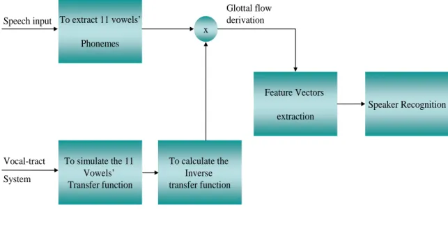
To extract 11 vowels’ Phonemes Speaker Recognition To simulate the 11 Vowels’ Transfer function To calculate the Inverse transfer function Feature Vectors extraction x Glottal flow derivation Speech input Vocal-tract System

Fig. 1-3 : Block Diagram of Glottal Flow Derivation

After extracting the glottal flow derivation, the features are applied to a speaker verification task using MFCCs feature vectors and a Gaussian Mixture Model (GMM). A speaker model which represents each speaker in the speaker recognition system will be built in the training phase and then be used for speaker matching in the test phase. The modeling approaches are various, including the artificial neural network (ANN) [7],[10], the vector quantization (VQ) [11],[12], the Gaussian mixture models (GMM) [13],[14], the hidden Markov model (HMM) [15],[16],[17] and so on. In 1995, Reynolds demonstrated that the GMM-based classifier works well in text-independent speaker recognition even with speech features that contain rich linguistic information like MFCCs [18]. GMM provides a probability model of the underlying sounds of speaker’s voice. It

(17)

uses several Gaussian density functions to model a speaker and each density function has

its own mean and covariance. For a feature vector denoted as x , the mixture density for _j

each speaker is denoted as

(

)

=

∑

M₌

( )

i j s i s i s j p x x p 1

|λ ω . Gaussian density function is defined as:

( )

_{( )}

(

)

( )

(

)

⎭ ⎬ ⎫ ⎩ ⎨ ⎧₋ ₋ _∑ ₋ ∑ = − i j i i j i D j s i x x x p µ µ π 1 ' 2 / 1 2 / 2 1 exp | | 2 1 (1.1)

The density is a weighted linear combination of M component uni-modal Gaussian

density each parameterized by a mean vector µr_is and covariance matrix ∑ . _is Collectively, the parameters of a speaker’s density model are denoted as

{

s

}

i s i s i s = ω ,µ ,∑

λ r and maximum likelihood (ML) estimates of the model parameters are obtained by using the expectation maximization (EM) algorithm. Therefore, for an utterance X =

{

X₁,...,X_N

}

and a reference group of speakers

{

S₁,S₂,...,S_s

}

represented by models

{

λ₁,λ₂,...λ_s

}

, the identification is executed by the maximum likelihood classification rule sˆ=argmax₁_≤_s_≤_S p

(

X |λ_S

)

which decides who the candidates speaker [19] is.

In the following, we will describe the framework of our proposed speaker recognition system briefly.

First, we choose 11 vowels from MAEDA’s vocal tract system, the 11 vowels are shown in Table 1-1. From the vocal tract simulation of the system, we can calculate the transfer function of each vowel then we can use it as an inverse filtering applied to the corresponding vowel grabbed from input sentences of the TIMIT database. In the next procedure, we choose the MFCCs as our feature since the mel-scale mimics the human hearing which is sensitive to the sound in low-frequency domain. After the feature of each frame has been extracted, we applied the vowels of each speaker to a ML-based GMM speaker verification system to construct a model for each speaker. The glottal flow

(18)

derivation method is to enhance the GMM model for considering the overall recognition system and reducing the system error rate. The detail of the MAEDA’s vocal tract system and overall speaker recognition system will be described separately in Chapter 2 and Chapter 3.

Table 1-1 : 11 Vowels with Inverse Filtering

0 1 2 3 4 5 6 7 8 9 10 11

None iy ey eh ah aa ao oh uw iw ew Oe

Organization of Thesis

This thesis is organized as follow: In Chapter 2 we will review MAEDA’s digital simulation method of the vocal-tract system. And in Chapter 3 we will describe the proposed structure of the speaker recognition, including MFCCs, glottal flow derivation with inverse filtering, and the GMM model classifier. We depict the used database and show the experimental results to verify that the glottal flow derivative conveys speaker identity information and the performance of our speaker recognition system in Chapter 4. Finally, we will give the conclusions of this thesis and the future work in Chapter 5.

(19)

2 Chapter 2

Framework of the Vocal-Tract System in

Speaker Recognition System

2.1 Introduction

This Chapter first describes qualitatively the properties of the components of glottal flow and its derivative, and then briefly reviews Shinji MAEDA’s theory in simulating the model of vocal tract and associated source/vocal tract interaction, and ends with a glottal flow derivative model for extracting features to be used in speaker recognition.

2.2 Properties of the Glottal Flow

Speech production is typically viewed as a linear filtering process which can be considered time invariant over short time intervals. The glottal flow volume velocity,

denoted by µ_g

( )

t , acts as the source, sometimes also referred to as the “glottal flow excitation,” to the vocal tract with impulse response h(t). The volume velocity output of the vocal tract is then modified by the lip impedance. Because the pressure/volume velocity relation at the lips can be approximated by a differentiator [20], the speech pressure waveform s(t) measured in front of the lips can be expressed as

( )

t

d

( ) ( )

t

h

t

dt

d

( )

t

dt

h

( )

t

s

≈

[

µ

_g

∗

]

/

=

[

µ

_g

/

]

∗

. The effect of radiation is typically included in the source function [20]; the source to the vocal tract, therefore, becomes the

(20)

( )

t

( )

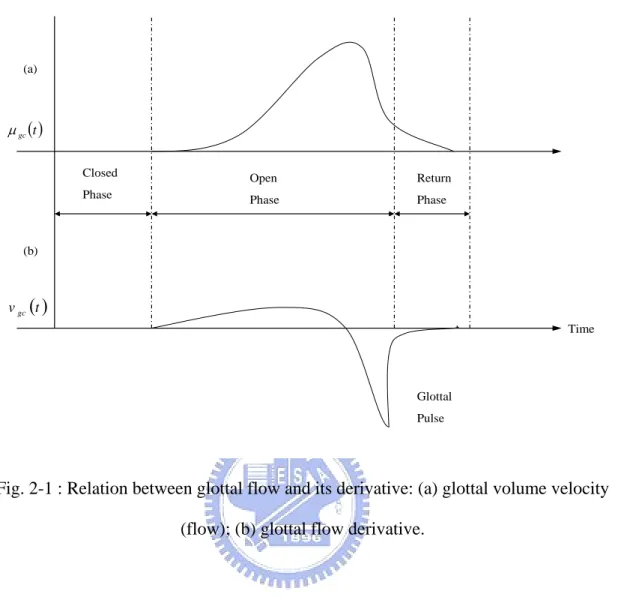
t

v_g =µ&_g . Following the approach of Ananthapadmanabha and Fant [21], we assume that the glottal flow and its derivative consist of coarse- and fine-structure components.

1) Coarse Structure: The relation between the coarse structure of the glottal flow,

denoted by µ_gc

( )

t , and its derivative, v_gc

( )

t , is shown in Fig. 2-1 for an idealized glottal flow function. In obtaining the glottal flow derivative, applying the lip radiation effect of the source flow, rapid closing of the vocal folds results in a large negative impulse-like response at glottal closure, called the glottal pulse, as shown in Fig. 2-1. The coarse structure represents the general shape of the glottal flow. The time interval during which the vocal folds are closed, and during which no flow occurs, is referred to as the glottal

closed phase. The time interval over which there is nonzero flow and the vocal folds are

fully or partially open is referred to as the glottal open phase. The time interval from the most negative value of the glottal flow derivative to the time of glottal closure is referred to as the return phase. The asymmetry of the glottal flow shape during the open phase, sometimes referred to as skew in the glottal flow, is due approximately in part to the manner in which the glottis changes in time, and in part to the loading by the vocal tract during the glottal open phase [21]. In this glottal flow model, the return phase is particularly important, as this determines the amount of high-frequency energy present in both the source and the speech. The more rapidly the vocal folds close, the shorter the return phase, result in more high-frequency energy and less spectral tilt.

(21)

(a) (b) Closed Phase Return Phase ( )t gc µ ( )t vgc Open Phase Time Glottal Pulse

Fig. 2-1 : Relation between glottal flow and its derivative: (a) glottal volume velocity (flow); (b) glottal flow derivative.

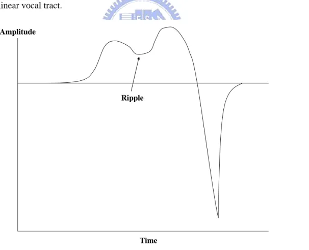
2) Fine Structure: Fine structure of the glottal flow derivative, denoted by ν_gf

( )

t , is the residual waveform obtained by subtracting the coarse structure from the glottal

flow derivative, i.e. ν_gf

( )

t =ν_g

( )

t −ν_gc

( )

t . Two contributions of fine structure are discussed in this section, ripple and aspiration. As illustrated in Fig. 2-2, ripple is a sinusoidal-like perturbation that overlays the coarse glottal flow, and thus the glottal flow derivative, and arises from the time-varying and nonlinear coupling of the glottal flow with the vocal tract cavity, due to primarily the vocal tract first formant [21]. The timing and amount of ripple is dependent on the configuration of the glottis during both the open and closed phases [21],[22],[23]. For example, with folds that open in a zipper-like fashion, ripple may begin at a low level early into the glottal cycle, and then grow as the

(22)

vocal folds open more completely.

Our second form of fine structure, aspiration at the glottis, arises when turbulence is created as air flows through constricted vocal folds, and is also dependent on the glottis for its timing and magnitude. For example, a long, narrow opening, which constricts the air flow along the entire glottal length, tends to produce more aspiration than, for example, a triangular-shaped opening with partial constriction. The creation of turbulence at the glottis is highly nonlinear and a satisfactory physical model has yet to be developed. A simplification is to model aspiration as a random noise process, which is the source to the linear vocal tract. The complete fine-structure source is modeled as the addition of the aspiration and ripple source components. But in this thesis, for the simplifications, we will only consider ripples and aspiration as a random noise process, which is the source to the linear vocal tract.

Amplitude

Time Ripple

Fig. 2-2 : Glottal flow derivative waveform showing coarse and ripple component of fine structure due to source/vocal tract interaction.

(23)

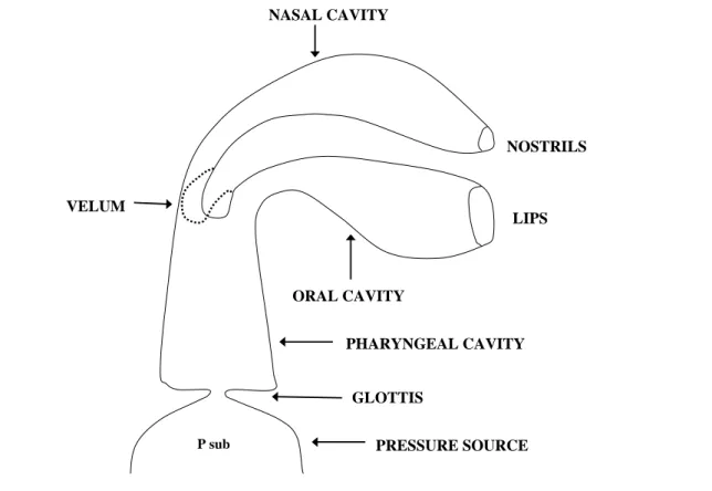
2.3 Physical Model of Vocal Tract

A model of the vocal-tract system under consideration is shown in Fig. 2-3, which oral, nasal cavities, and pharyngeal is included. The innermost end of the pharyngeal tube is a pressure source through the narrow constriction representing the glottal orifice. The tracheal tube is omitted in this simulation, since the effects on the acoustic effect upon the speech spectrum seems to be not so important, except for unvoiced sounds where the glottal opening is fairly large enough [24],[25]. Universally, it’s almost accepted that the acoustic waves inside the vocal tract can be regarded as plane or one dimensional for frequencies below 4 kHz. So, only the cross-sectional area and the perimeter along the length of the vocal tract determine the acoustic characteristics. Furthermore, if the cross-sectional shapes can be assumed to be uniform, for example, as circular, the area function A ,

( )

x t , as shown in Fig. 2-4, determines completely the acoustic properties of the vocal tract. The area function A'

( )

x,t

specifies that of the nasal tract. The entities related to the nasal tract are marked by the prime ‘/’. And in this thesis, all the assumptions introduced in Chapter 3 are based on the uniform vocal tract as circular.

The pressure p ,

( )

x t and the volume velocity u_g

( )

x, inside an acoustic tube with t

non-rigid walls are governed, in the first order approximation, by the following partial differential equations; the equation of Motion (EQM), the continuity (EQC), and that of wall vibration (EQW), shown as below

0 0 0 0 ₊ ₌ ∂ ∂ + ∂ ∂ A ru A u t x p ρ g g (2.1) 0 0 0 2 0 0 = ∂ ∂ + ∂ ∂ + ∂ ∂ + ∂ ∂ t y S t A c p A t x u_g ρ (2.2) 0 2 2 = + ∂ ∂ + ∂ ∂ ky t y b t y m (2.3)

(24)

Respectively, in eqs., (2.1) and (2.2), ρ₀ and c indicate that density of the air at equilibrium, and the sound velocity. The area function is denoted by A₀

( )

x,t , which is related to the previously defined area function A

( )

x,t by

( )

x

,

t

A

₀

( )

x

,

t

y

( )

x

,

t

S

₀

(

x

,

t

)

A

=

+

(2.4)

where S₀

( )

x,t indicates a given perimeter of the vocal tract, and y

( )

x,t the amplitude of the yielding of walls due to the sound pressure inside the tube.

VELUM PRESSURE SOURCE P sub GLOTTIS PHARYNGEAL CAVITY ORAL CAVITY LIPS NOSTRILS NASAL CAVITY

Fig. 2-3 : A schematized vocal-tract model.

The equation of walls, eq. (2.3) has been derived assuming that walls are locally reacting, i.e., the motion, normal to the surface, of one portion of the walls is dependent only upon the acoustic pressure on that portion and independent of the motion of any other part of the walls. The coefficients m, b, and k in eq. (2.3) respectively represent the mass, mechanical resistance, and the stiffness of the wall per unit length of the tube.

(25)

These coefficients, for simplification, are assumed to be constant and uniform along the vocal tract, even though that the actual values vary according to the location and also the tenseness of the muscles beneath the wall surface [26],[27]. Often in the literature, these constants have been specified in terms of a unit surface area. In such cases, the total mass of the walls may vary unrealistically depending on the vocal tract configuration. On the contrary, in the specification per unit length, the total mass should be kept relatively constant, since the length variation of the tract is relatively small, especially in comparison with the surface area variation. Considering the fact that the total mass of the vocal tract system is constant, we feel that the specification of mass per unit length seems to be more reasonable than its counterpart. We have discussed only the mass coefficient, since the mass is the dominant component of the non-rigid walls in terms of its acoustic consequences, The values of these constants are estimated from the data reported by [26], assuming the cross-sectional area of 4 2

cm .

This is a rather crude representation of the non-rigidity of vocal-tract walls. Nevertheless, this approximation should be able to account for the dispersive propagation of acoustic waves and for an increase in the bandwidth of the formants due to the loss of energy through the mechanical resistance of low frequencies.

The flow resistances only become relevant at an extremely narrow constriction. Such a constriction is formed at the glottis during the production of voiced or aspired sounds, and at the place of articulation along the vocal tract during the production of certain consonants. And the resistance at the glottal orifice has been investigated by [28]. They formulated the total resistance as:

2 0 3 2 2 12 g g c g g g g A u k X A l R = µ + ρ (2.5)

(26)

cross-sectional area, the length, and the thickness, respectively, of a rectangular duct representing the glottal orifice, and k is a coefficient having a typical value of 1.38, it’s _c

determined to account for a normal condition of the larynx being about 3 mm thick. In eq. (2.5), the first term represents a laminar resistance due to the viscosity of the air, and

the second term represents a kinetic loss, which depends on the volume velocity u . _g

Because of an abrupt contraction and expansion in the passage of airflow at the glottis, eddies are formed at its inlet and outlet. In fact, the value of the coefficient k in eq. (2.5) _c

varies from 0.05 to 0.5 at the inlet, and from 0.2 to 1.0 at the outlet, depending on the shapes.

In the case of a constriction along the vocal tract, the shape of the constriction may be so different from the larynx that eq. (2.5) is no longer valid. In addition, the shape of the constriction would vary significantly, depending on the manner of articulation. In this implementation, we abandoned this constriction. Instead, a formula for a laminar resistance in a circular duct is used. The resistance per unit length is given by

2

/

8 A

R = πµ (2.6)

where A indicates the cross-sectional area of the circular duct.

In Fig. 2-3, the glottal end of the pharyngeal tube is directly connected to the pressure source. The boundary condition is represented by

( ) ( )

t

p

x

t

P

_sub

=

₀

,

(2.7)

where P indicates a give sub-glottal air pressure, and _sub x is the coordinate value of ₀

(27)

0 0 A’( x,t ) A ( x,t ) GLOTTIS X’ X

NASAL BRANCHING LIPS M X K X Nostrils N X '

Fig. 2-4 : The ideal function of the time-varying vocal tract.

The location of the nasal coupling point is defined as x=x_k in Fig. 2-4. The boundary condition of volume velocity and the pressure must satisfy the following equations

( ) ( )

x

t

u

x

t

u

( )

t

u

_k−

,

=

_k+

,

+

'

0 ,

(2.8)

)

,

0 (

'

)

,

(

)

,

(

x

t

p

x

t

p

t

p

_k−

=

_k+

=

(2.9)

Where the superscript ‘-’ indicates the pharyngeal end, and ‘+’ means the inlet of the oral cavity.

The outlet of the oral and nasal tract is connected to a space where sound is radiated. Since we don’t concern with the propagation of sound in the radiation filed in this thesis, it should suffice to characterize the space as an acoustic load specifying the velocity-pressure relationship at the mouth opening and at the nostrils. Morse and Ingard [29] have formulated the radiation load as an impedance composed of a resistance and an inductance in series. The resistance is proportional to ω2

(28)

implement into the time-domain simulation. Fortunately, Flanagan [30] has suggested the parallel circuit approximation, where both the conductance, G_rad, and the susceptance,

rad

S , are independent of frequencies. Thus, at the lip opening and at the nostrils, we obtain the following boundary condition

(

)

=

_∫

( ) (

)

+

( ) (

)

t M rad M rad M

t

S

t

p

x

t

dt

G

t

p

x

t

x

u

0

,

_(2.10) where S_rad

( )

t =9πA₀

(

x_M,t

)

/128ρ₀c G_rad

( )

t =3π πA₀

(

x_M,t

)

/8ρ₀

Considering that we don’t know exactly how to describe the real lip opening shapes, nor their acoustic effects, it may not be justifiable to further elaborate the specification of the radiation load on the basis of the circular vibrating piston equivalent.

2.4 Frequency Response of a Uniform Tube

For a given configuration, the simulation results can be evaluated in terms of the transfer function of the discrete time system. For calculating the transfer function, we derive an impulse response of the system as the pressure variation at the mouth opening when the system was excited by abruptly closing the glottal section after a steady airflow had be created in the glottis. The situation of acoustic wave propagates in the vocal tract is shown in Fig. 2-5. The horizontal axes indicate time in millisecond. The curve at the top, marked by ‘AG’, represents a stepwise variation of the glottal area. At t = 5ms, the glottal area is closed instantaneously. The second curve, marked by ‘UG’, represents the glottal airflow as a function of time. At t = 0, the sub-glottal are pressure (8cm H2O) is

applied to create the airflow. Notice that the glottal flow increases with time, but with some oscillatory components, indicating the influence of the vocal tract resonances.

(29)

About 3 ms later, the oscillation has been completely suppressed, primarily because of the loss of energy through the glottal resistances, and the flow reached a steady state. The airflow drops abruptly to zero at the instant of the glottal closure, which causes a sudden pressure drop at the pharyngeal end of the vocal tract, as shown at ‘P6’ in Fig. 2-5. ‘P6’ is corresponding to 3cm above the glottis, and ‘P36’ to the mouth opening. From ‘P11’ to ‘P31’ along the vocal tract are intermediate points with equally spaced intervals of 2.5cm. It indicates that the sudden pressure drop propagates toward the mouth opening. At the exit of the tube, the negative pressure is immediately reflected back inside the tube so that a sharp negative impulse-like peak is formed at the beginning. The ringing following the first several pulses in the manifestation of Gibbs’ phenomenon, due to the fact that the frequency bandwidth of the discrete system is finite. After several reflections of the pressure wave, the high frequency components are sufficiently damped out and the ringing effect disappears as well as the marked impulse-like pressure peaks.

(30)

Fig. 2-5 : A given step function for the glottal area (AG), the calculated glottal airflow (UG), and acoustic pressures at different places (From P6 to P36) along the uniform tube.

The frequency response obtained by applying the discrete Fourier Transfer to the pressure waveform at the mouth opening can be regarded as the transfer function of the vocal tract in the closed glottis condition. In our implementation, all the transfer functions of vowels are defined when the glottis is closed.

There are some examples of the impulse response and their corresponding frequency response of a uniform tube with 5cm in a cross-sectional area and 162 cm in length are shown as below

(31)

Fig. 2-6 : The impulse and frequency response of a uniform tube. Those from the simulation with fs =40kHz and X = 1cmare plotted by the solid line as a reference.

The frequency response with fs =20kHz is indicated by the dotted line.

Fig. 2-7 : The impulse and frequency response of a uniform tube. Those from the simulation with fs =40kHz and X = 1cm are plotted by the solid line as a reference.

(32)

2.5 Frequency Response of Vowels

Mrayati [31] has calculated the transfer function of the vocal tract for 11 different French vowels by means of the transmission-line analog of the tract as described here. In his experiment, the transfer functions were computed directly in the frequency domain, and the area functions, the frequencies and the bandwidths of the first three formants of the 11 vowels are reported. So, there are some comparison results between the two methods; one in the frequency domain (FDS) and the other in the time domain (TDS).

The area functions are described by a piecewise-constant function having a fixed section length of 1cm (i.e., X = 1cm). The sampling rate of 40 kHz or 20 kHz is used in TDS method. The impulse and frequency response for the vowel /a/ simulated with

kHz

f_s =40 is shown in Fig. 2-8.

The formant frequencies computed in TDS agreed well with those in FDS method, except for the first formant (F1) of the vowel /i/. The value of the F1 frequency is 268 Hz, which is about 10% higher than the 224 Hz calculated in FDS method. The difference seems to be attributed to the different manner of specifying the walls of vocal tract. The parameters, m, b, and k in eq. (2.3) make per unit length in TDS tend to result in lower wall impedance that that per unit area in FDS, for this particular vowel having sections with a large area. For the other vowels, the difference in F1 frequency is less than 5% and typically 2%, which means below difference limens (DL) of F1 frequencies. The difference limens for the first and second formants are about 3% to 5% [30].

The discrepancy in the second (F2) and third formant (F3) frequencies in the two methods was quite small and never exceeded 1.5%, when f_s =40kHz is used. A closed observation has indicated, however, that F3 frequencies in TDS are always slightly lower than the corresponding F3 in FDS, indicating the trace of the frequency warping in TDS. The effect of the warping on the F3 frequencies become quite noticeable as f_s =20kHz

(33)

is used. In this case, the F3 frequencies in TDS were typically 4% and as much as 7% below the corresponding F3 in FDS. Since this simulation is workable and the error rate is pretty low, we use the 11 vowels’ transfer function calculated in the TDS method as our basis to estimate the glottal flow excitation for our speaker recognition system. The simulation method will be discussed later in Chapter 3.

(34)

Fig. 2-8 : The impulse and frequency response of the vowel /a/ simulated with

kHz

(35)

3 Chapter 3

Speaker Recognition System by Using

Inverse Transfer Function of Vocal Tract

System

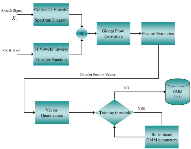
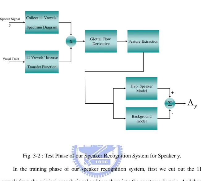
3.1 Overall Speaker Recognition System

The framework of our overall speaker recognition system is shown in Fig. 3-1 and Fig. 3-2. Vector Quantization Collect 11 Vowels’ Spectrum Diagram 11 Vowels’ Inverse Transfer Function Glottal Flow Derivative X Feature Extraction Speech Signal Vocal Tract > Training threshold? NO YES GMM (λs) s X

26 order Feature Vector

Re-estimate GMM parameters

(36)

Collect 11 Vowels’ Spectrum Diagram 11 Vowels’ Inverse Transfer Function Glottal Flow Derivative X Feature Extraction Background model Hyp. Speaker Model ∑

Λ

Speech Signal y Vocal Tract + -y

Λ

Fig. 3-2 : Test Phase of our Speaker Recognition System for Speaker y.

In the training phase of our speaker recognition system, first we cut out the 11 vowels from the original speech signal and turn them into the spectrum domain. And then we calculate the corresponding inverse transfer function of the vowel from the vocal tract simulation system mentioned in Chapter 2. After multiplying the spectrums from the original speech signal and the inverse transfer function of the vocal tract frame by frame, we can obtain the glottal flow derivative known as the simple equation below

( )

ω E

( )

ω H

( )

ω S = × (3.1)

( ) ( )

ω ₌ ω _×

( )

ω −1 H S E (3.2)

where E

( )

ω represents the glottal flow derivative, H

( )

ω represents the transfer function of the vocal tract, and S

( )

ω indicates the speech signal in the frequency domain. After obtaining the glottal flow derivative, we extract the MFCC and other

(37)

features, which are usually used in speaker recognition system from the glottal flow derivativeE

( )

ω . After vector quantization, we set a training threshold equals 0.005 to determine that the GMM parameters are well calculated or not. If the training rate is greater than training threshold, the GMM parameters will be re-calculated and the iteration will continue. If not, the GMM parameters will be saved and be used by the test phase as the background model. From the above steps, we can obtain the Gaussian Mixture Model of speaker s in the training phase.

In the test phase, we also calculate the 11 vowels’ glottal flow derivative from the same steps mentioned in training phase from the speech signal. Still we extract the MFCC feature of the speech signal and use the feature vectors to rebuild other Gaussian Mixture Model and parameters. In the testing phase, we compare the hypothesis GMM model parameters with the background GMM model parameters and use the equation below the determine the score of speaker y

( )

y

=

log

p

(

y

|

λ

hyp

)

−

log

p

(

y

|

λ

_hyp

)

Λ

(3.3)

The speaker evaluation system is shown in Fig. 3-3. After we calculate all the scores of speakers, we use the speaker evaluation system to find equal error rate and the threshold for all of the speakers according to the statistic method called Receiver Operating Characteristic (ROC). The speaker evaluation system will read the login and impostor scores separately, and estimates the ROC curve by 500 times iteration. The Resolution Scale here is 500, and we can adjust the value in our program. When the threshold is decided, the evaluation system judges the scores of speakers to decide the speaker is our customer or just an impostor. If the score is smaller than threshold, the system rejects the speaker and takes him/her as impostor, on the contrary, the system accepts the speaker and take him/her as a customer.

(38)

y

Λ

500 iterations to Find

EER and Threshold

> Threshold? Yes No Reject Accept Customer Impostor 1

Λ

……..

Fig. 3-3 : Speaker Evaluation System

3.2 Each Block of Speaker Recognition System

In the section, we will decompose the entire speaker recognition system into blocks. After that, we will detail each block of the recognition system.

3.2.1 Glottal Flow Derivative

In this block, it actually combines two sub-blocks including collection of vowels’ spectrum diagram and vowels’ inverse filtering function. We will introduce the two parts step by step.

In the inverse filtering sub-block on the left side of Fig. 3-4, we can obtain the vowels’ transfer function and frequency response from simulating the 11 vowels’ vocal

(39)

tract configuration mentioned in Chapter 2. After inverse filtering, we can obtain H

( )

ω −1

(Inverse Transfer Function), and H

( )

ω −1 will be substitute into equation (3.2) in order to get the glottal flow derivativeE

( )

ω .

In the collection of vowels’ spectrum diagram sub-block on the right side of Fig. 3-4, first, we cut off the specific vowels in Table 1-1 out from the speech utterances of TIMIT database. After that, we remove the DC-offset in the output waveform by using offset compensation, and then the signal is pre-processed by a high-pass filter. Next, the speech signal is passed through a Hamming Window and we will cut into segments (frames). In order to match up the data frame after inverse filtering, we should transform the speech signal frames to the frequency domain via the Fast Fourier Transform. The data is

(40)

DC_offset Extracting 11 vowels Speech Signal s X Hamming Window Pre_emphasis FFT Frame Maker Inverse filtering Corresponding vowels’ Transfer function X Vocal tract Simulation

Glottal Flow Derivative

Fig. 3-4 : Block Diagram of Glottal Flow Derivative.

3.2.2 Feature Extraction

MFCC is widely used in the automatic speech recognition (ASR) applications. It is primarily for three reasons [32]: 1) The cepstral features are roughly orthogonal because of the discrete cosine transformation (DCT), 2) cepstral mean subtraction eliminates static channel noise, and 3) MFCC is less sensitive to additive noise than linear prediction cepstral coefficients (LPCC). The key component of MFCC responsible for noise robustness is the filter bank; the filters smooth the spectrum, reducing variation due to additive noise across the bandwidth of each filter.

(41)

data of the collection of vowels’ spectrum diagram sub-block. So, in our feature extraction block, we extract 26 order features. First, the spectrum data of the glottal flow derivative is passed through a 12 order Mel frequency cepstral coefficients filter. And then the spectrum data is passed through 8 order delta-cepstral coefficients filter and 4 order delta-delta-cepstral coefficients filter. Finally, we will let the data pass through 1 order delta-energy and 1 order delta-delta-energy filter banks and we use the cepstral mean subtraction (CMS) in order to eliminate the tunnel effects. The block of feature extraction is shown in Fig. 3-5.

Feature Extraction

1-order delta-energy & 1-order delta-delta-energy

8-order delta-cep & 4-order delta-delta-cep 12-order MFCCs Build GMM Model Glottal Flow Derivative Speech Signal s X GMM (λs) Feature extraction begins CMS Training Vectors

(42)

3.2.3 Build GMM Model of Training Phase

For determining the speaker identification of our source features, we use a Gaussian mixture model (GMM) speaker identification system. Each Gaussian is assumed characterized by a diagonal covariance matrix. This choice is based on the empirical evidence that diagonal matrices outperform full matrices and the face that the probability density modeling of an Nth-order full covariance mixture can equally well be achieved using a larger order, diagonal covariance mixture. Maximum Likelihood speaker model parameters are estimated using the iterative expectation-maximization (EM) algorithm. Here, we use some equations to symbolize the algorithm.

(

)

=

_∑

M₌

( )

i j s i s i s j p x x p |λ ₁ω (3.4)

( )

_{( )}

(

)

( )

(

)

⎭ ⎬ ⎫ ⎩ ⎨ ⎧₋ ₋ _∑ ₋ ∑ = − i j i i j i D j s i x x x p µ µ π 1 ' 2 / 1 2 / 2 1 exp | | 2 1 (3.5) ( )

(

k

)

(

( )k

)

X

p

X

p

|

λ

+1

>

|

λ

(3.6)

where eq. (3.4) indicates the mixture density, and eq. (3.5) indicates Gaussian density function, eq. (3.6) represents to iterate the best parameters for Maximum Likelihood (ML) by Expectation-Maximization (EM) algorithm.

The use of the GMM classifier is justified by its being an established, general classifier, which assumes predetermined distributions, and nonparametric classifiers which typically are computationally expensive, such as K-Nearest Neighbors [33],[34]. Another advantage is that it is insensitive to the temporal change when used in text independent task. It is well known that if the number of component densities in the mixture model is not limited, we can approximate virtually any “smooth” density.

The input training vectors (X) in our system can be represented by

(

)

_∑

(

)

= = T t t x p X p 1 | log |

(43)

algorithm. Finally, we can obtain the GMM model parameters of the training set after the iteration progress of the EM algorithm. The block flow chart of Build GMM Model for training phase and test phase are shown separately in Fig. 3-6 and Fig. 3-7.

Feature Extraction Build GMM Model Glottal Flow Derivative Speech Signal s X GMM (λs) Build GMM Model begins Expectation-Maximization (EM) Training Vectors (Xs) GMM (λs) Iteration End? NO YES

(44)

Feature Extraction Scoring Glottal Flow Derivative Speech Signal X > threshold? YES NO Customer s Impostor Score begins Build GMM Model λ Test Vectors (X) Comparison wit Background Model Score

(45)

4 Chapter 4

Experiment Results and Discussion

4.1 Introduction

In the previous chapter, we described the structures of the proposed speaker recognition system. For investigating and showing the contribution and verification of these methods we applied, several sets of experiments were done. There are thirteen sets of experiment in total, and two subsets of experiment result are included in each experiment. In the first part of experiments, we evaluated the effects glottal flow derivative in a single region with ML-based GMM with MFCC features, the results are separated by eight regions. In subset I, we give the results which the speech signals were processed by our proposed scheme. On the contrary, in subset II, we give the results of 11 vowels which we used the same features and classifier but without processed by our glottal flow derivative method. That means we cut of the 11 vowels from a speaker’s utterances and directly send them into the feature extraction parts and build they own Gaussian Mixture Model just as the traditional ways of speaker recognition does. We did these subsets of experiment in order to verify the assumptions we had made and to show the efficiency of our proposed scheme. In the second part of experiments, we used a random number of impostors across the 8 dialect regions to evaluate the effects when our scheme was used in different dialect regions. And in the last part of experiments, we give results of the cases when we focus on some security control system, such as an entrance guard system, we can adjust the threshold or change the dimensions of feature vectors to reduce the error rate. The experimental results showed the contribution of this model.

(46)

For these experiments, several processing steps occur in the front-end speech analysis. First, the speech signal was decomposed in frames of 256 samples with an overlap of 128 samples (the sampling rate is 16k Hz). For each frame, FFT was computed and provided the square values of the original sample values representing the short term power spectrum in the 0~4k Hz band. And then, this Fourier power spectrum was used to compute the power accumulated in each filter bank and the discrete cosine transformation (DCT) to get the cepstral coefficients called MFCC with 12 orders.

4.2 Experiment Database

The database for the experiments is the TIMIT acoustic-phonetic speech corpus. This corpus is widely used throughout the world and provides a standard that permits direct comparison of experimental results obtained by different methodologies. In this thesis, we used the entire corpus of TIMIT database including 8 dialect regions. Table 4-1 shows the number of speakers for the 8 dialect regions, broken down by sex. There are 10 sentences spoken by each of 630 speakers from 8 major dialect regions of the United States. In the first eight sets of experiment, there are two subsets .In subset I, we chose 9 sentences to train, the rest of 1 sentence for login test and the other speakers of the same region for impostors. In experiments subset II, we will create exactly the same conditions of subset I but without processed with the inverse filtering process obtained from glottal flow derivative estimate, this subset of experiment are used for comparison. In the ninth to eleventh experiments, we randomly chose a number of speakers for training and the other as impostors which across dialect regions were chosen for impostor test. In the last two experiments, we give the results to show that we can achieve high performances by using our proposed scheme.

(47)

Table 4-1 : Dialect Distribution of Speakers

Dialect Region (dr) # Male # Female Total dr1: New England 31 (63%) 18 (27%) 49 (8%) dr2: Northern 71 (70%) 31 (30%) 102 (16%) dr3: North Midland 79 (67%) 23 (23%) 102 (16%) dr4: South Midland 69 (69%) 31 (31%) 100 (16%) dr5: Southern 62 (63%) 36 (37%) 98 (16%) dr6: New York City 30 (65%) 16 (35%) 46 (7%) dr7: Western 74 (74%) 26 (26%) 100 (16%) dr8: Army Brat 22 (67%) 11 (33%) 33 (5%)

8 438 (70%) 192 (30%) 630 (100%)

4.3 Experiment Results

In the following, three sets of experiments would be carried out to evaluate and verify our recognition system.

We assigned one class to each of features, and after the process of voting by the classifications of features, we would make sure which person the speaker was. The recognition rate was calculated by the result of the error classification.

(48)

Part I – Experiment 1

Fig. 4-1 : Sketch of the feature and the GMM model of Experiment Part I

Subset I

Table 4-2 : Recognition Results of Subset I for 1 Customer (48 impostors) Code Book Size FR_NO. FA_NO. EER

32 Bits 22/49 1033/2352 44.4090130% 64 Bits 30/49 431/2352 39.7746600%

Subset II

Table 4-3 : Recognition Results of Subset II for 1 Customer (48 impostors) Code Book Size FR_NO. FA_NO. EER

32 Bits 22/49 1039/2352 44.5365640% 64 Bits 15/49 1154/2352 39.8384360%

In these tables, “Code Book Size” means how many bits we used to store the code vectors; “FR_NO.” means the number of false rejection and it is represented in the way of “FR_NO./Total Sentences” so as the FA_NO. is represented; “FA_NO.” means the number of false alarm; and “EER” means the equal error rate, it is the average of false rejection rate and false alarm rate.

Dr1 to Dr8 MFCC

ML-Based GMM

(49)

Part I – Experiment 2

Subset I

32 Bits 38/102 3890/10211 38.6755375% 64 Bits 42/102 4378/10211 42.0259015%

Subset II

32 Bits 45/102 4353/10211 43.3740720% 64 Bits 12/102 8446/10211 47.2397125%

Part I - Experiment 3

Subset I

32 Bits 38/102 4099/10302 38.5216455% 64 Bits 35/102 4702/10302 39.9776737%

Subset II

32 Bits 41/102 4199/10302 40.4775770% 64 Bits 22/102 6359/10302 41.6472535%

(50)

Part I - Experiment 4

Subset I

32 Bits 40/100 3914/9900 39.7676770% 64 Bits 43/100 4271/9900 43.0707070%

Subset II

32 Bits 42/100 3871/9900 40.5505055% 64 Bits 22/100 6187/9900 43.2474755%

Part I - Experiment 5

Subset I

32 Bits 39/98 3721/9506 39.4698200% 64 Bits 31/98 4532/9506 39.6539035%

Subset II

32 Bits 44/98 4308/9506 45.1083530% 64 Bits 44/98 4180/9506 44.4351145%

(51)

Part I - Experiment 6

Subset I

32 Bits 19/46 583/2000 41.9771730% 64 Bits 21/46 889/2000 45.0510875%

Subset II

32 Bits 21/46 901/2000 45.3510880% 64 Bits 22/46 1019/2000 49.3880450%

Part I - Experiment 7

Subset I

32 Bits 38/100 3874/9900 38.5656570% 64 Bits 34/100 4872/9900 41.6060610%

Subset II

32 Bits 43/100 4295/9900 43.1919205% 64 Bits 43/100 4331/9900 43.3737385%

(52)

Part I - Experiment 8

Subset I

32 Bits 13/33 426/1056 39.8674250% 64 Bits 15/33 471/1056 45.0284095%

Subset II

32 Bits 14/33 442/1056 42.1401515% 64 Bits 4/33 865/1056 47.0170465%

In order to verify that our proposed scheme is stable and the glottal flow derivative indeed convey the speaker identification information, the eight experiments above used all the speakers in the TIMIT. The eight experiments were taken by different dialect regions of the United States, in order to verify the efficiency of our scheme applied to different regions, we mixed the dialect regions together with a random number of speakers in the following three experiments shown as below:

(53)

Part II - Experiment 9

Fig. 4-2 : Sketch of the feature and the GMM model of Experiment Part II

Subset I

32 Bits 43/95 4108/8930 45.6326990% 64 Bits 58/95 2478/8930 44.4008960%

Subset II

32 Bits 44/95 4088/8930 46.0470320% 64 Bits 17/95 6960/8930 47.9171325%

Here, the meaning of mixing of the dialect regions represents that we chose a random number of speakers across the eight dialect regions of the TIMIT database. This part of experiments was set to verify the effects of our proposed scheme applied to across different regions. Mixing of the dialect regions MFCC ML-Based GMM

(54)

Part II - Experiment 10

Subset I

32 Bits 30/84 2578/6972 36.3453825% 64 Bits 24/84 3777/6972 41.3726345%

Subset II

32 Bits 36/84 3048/6972 43.2874350% 64 Bits 37/84 3033/6972 43.7750995%

Part II - Experiment 11

Subset I

32 Bits 30/84 2711/6972 37.2991980% 64 Bits 35/84 2952/6972 42.0037288%

Subset II

32 Bits 34/84 2855/6972 40.7128515% 64 Bits 67/84 593/6972 44.1336770%

基於模擬聲門來源波型之語者辨識系統與確認技術

國 立 交 通 大 學

電機與控制工程學系

碩 士 論 文

基於模擬聲門來源波型

之語者辨識系統與確認技術

A Text-independent Speaker Recognition System

based on the Modeling of the Glottal Flow

Derivation Waveform

研 究 生：游家昇

指導教授：林進燈 博士

基於模擬聲門來源波型之語者辨識系統與確認技術

A Text-independent Speaker Recognition System based on

the Modeling of the Glottal Flow Derivation Waveform

研 究 生：游家昇 Student：Chia-Shen Yu

指導教授：林進燈 博士

Advisor：Dr. Chin-Teng Lin

國立交通大學

電機與控制工程學系

碩士論文

A Thesis

Submitted to Department of Electrical and Control Engineering

College of Engineering and Computer Science

National Chiao Tung University

in Partial Fulfillment of the Requirements

for the Degree of Master

in

Electrical and Control Engineering

July 2006

Hsinchu, Taiwan, Republic of China

中華民國 九十五 年 七 月

基於模擬聲門來源波型

之語者辨識系統與確認技術

學生：游家昇

指導教授：林進燈 博士

國立交通大學電機與控制工程研究所

中文摘要

A Text-independent Speaker Recognition System

based on the Modeling of the Glottal Flow Derivation

Waveform

Student: Chia-Shen Yu

Advisor: Dr. Chin-Teng Lin

Department of Electrical and Control Engineering

National Chiao Tung University

Abstract

誌謝

Contents

List of Tables

List of Figures

1 Chapter 1

Introduction

1.1 Motivation

1.2 Literature Survey

(

)

∑

( )

( )

( )

(

)

( )

(

)

{

}

{

}

{

}

{

}

(

)

Organization of Thesis

2 Chapter 2

Framework of the Vocal-Tract System in

Speaker Recognition System

2.1 Introduction

2.2 Properties of the Glottal Flow

國立交通大學

碩士論文

研究生：游家昇

指導教授：林進燈博士

研究生：游家昇 Student：Chia-Shen Yu

指導教授：林進燈博士

中華民國九十五年七月

指導教授：林進燈博士

_{( )}