以競價拍賣新股上市資料驗證新股折價與承銷商市場佔有
率關係
研究成果報告(精簡版)
計 畫 類 別 : 個別型 計 畫 編 號 : NSC 99-2410-H-004-065- 執 行 期 間 : 99 年 08 月 01 日至 100 年 07 月 31 日 執 行 單 位 : 國立政治大學財務管理學系 計 畫 主 持 人 : 姜堯民 公 開 資 訊 : 本計畫可公開查詢中 華 民 國 100 年 12 月 19 日
競價拍賣新股上市中的角色,結果發現:(1)承銷商的市場佔 有率與所承銷案件的折價程度呈現正向關係,(2)承銷商後續 承銷案件的期初報酬並不會愈來愈低,(3)承銷商相關的自營 生交易並不會影響新股上市的長期績效。承銷商在競價拍賣 新股上市中並沒有分配股數及訂價的權利,是以承銷商沒有 動機去穩定股價。 中文關鍵詞: 競價拍賣,新股上市,折價,自營商,拍賣次數
英 文 摘 要 : Taiwan has 90 IPO auctions during 1995-2003. It is one of only a few reasonably large samples of IPO auctions in the world, since most of the more than 20 countries that have used this method have dropped it relatively quickly. The dataset allows us to examine how underwriters behave to keep their market shares: (1) Unlike book building IPOs, in auction IPOs, the relationship between underwriter market share and IPO’s underpricing is positive, the higher
underpricing, the larger market share. (2) There is evidence that initial return of an underwriter’s high order IPO will be lower. (3) Underwriters’ affiliated dealer did not trade to push up IPOs’ long run return. In summary, underwriters of auction IPOs behave differently from underwriters of book-building IPOs. Since underwriters in auction IPOs have no pricing or allocation discretion ability, they do not have incentive to stabilize IPOs’ performance.
Underwriters pricing off the line lose no clients – evidence
from auction IPOs
Yao-Min Chiang
Department of Finance, National Chengchi University Email: [email protected]
Underwriters pricing off the line lose no clients – evidence from
auction IPOs
Yao-Min Chiang
Abstract
Taiwan has 90 IPO auctions during 1995-2003. It is one of only a few reasonably large samples of IPO auctions in the world, since most of the more than 20 countries that have used this method have dropped it relatively quickly. The dataset allows us to examine how underwriters behave to keep their market shares: (1) Unlike book building IPOs, in auction IPOs, the relationship between underwriter market share and IPO’s underpricing is positive, the higher underpricing, the larger market share. (2) There is evidence that initial return of an underwriter’s high order IPO will be lower. (3) Underwriters’ affiliated dealer did not trade to push up IPOs’ long run return. In summary, underwriters of auction IPOs behave differently from underwriters of book-building IPOs. Since underwriters in auction IPOs have no pricing or allocation discretion ability, they do not have incentive to stabilize IPOs’ performance.
Keywords: IPO, Auction, Market Share, Underpricing, Auction Order, Affiliated
1. Introduction
Underwriters in auction IPOs have no discretion or pricing ability. They seem have
no obligation or incentive to stabilize auction IPOs’ performance. According to
Beaty and Ritter (1986), in book-building IPOs, underwriters will gain less market
share if they set a lower offering price. There is a negative relationship between
underwriter’s market share and IPOs’ initial return. The reason behind this is that,
with higher underpricing, issuing firms will receive lower proceeds. This will make
the underwriter less attractive to potential issuing firms. Will underwriter in auction
IPOs follow the same strategy? That is the first issue I want to test in this paper.
For auction IPOs, if the relationship between market share and underpricing is
positive, it means that underwriters will try to attract more informed traders to bid,
and later auction’s initial return will be higher. If the relationship is negative,
underwriters will attract more uninformed investors to bid and the initial return for
later auction will be lower. The second objective in this paper is that I therefore
want to test the performance of frequent underwriters. If underwriters have the
obligation and incentive to stabilize IPO’s performance, they will try every method to
push up IPO’s return. I test whether trade from underwriters’ affiliated dealers can
affect an IPO’s long run return or not.
Beatty and Ritter (1986) find that abnormal first-day returns have a negative
effect on investment bank market share. However, Beatty and Welch’s (1996)
document a changing relationship between underwriter prestige and initial returns
(negative in the 1980s, positive in the 1990s). In particular, high underpricing
underwriters appear to be gaining prestige as they gain market share. Hoberg (2007)
argues that more underpricing underwriters attract more institutional clients. Based
on information compensation theory, underwriters will lower offering price to
underwriters continue to underprice to attract more informed clients and to make sure
the subscription will be fulfilled. Hoberg argues this underwriter persistence is
indeed driven by information asymmetry.
However, there will be a different story for auction IPOs. Underwriter with
previous high initial return will attract more bidders in later auctions. However,
underwriters attract more individual bidders rather than institutional bidders. Based
on Sherman (2005) and Chiang, Qian, Sherman (2009), more individual bidders’ entry
will push up clearing price and therefore lower initial return. So, higher previous
initial return attracts more clients, while most are individual investors, and gain more
market shares. More entry of individual bidders lowers initial returns in later
auctions. Lower initial returns become less attractive to investors, and then harm
underwriter’s market shares. This is also one of the reasons that auction approach
becomes less popular in IPO market.
The effect underwriters’ pricing strategy on market shares between book-building and
auction IPOs can be described as below.
For book-building IPOs, with higher previous initial returns, underwriters will
attract more informed traders to subscribe and to provide information. The result is
that underwriters will gain more market share and higher initial return for later IPOs.
For auction IPOs, with higher previous initial returns, underwriters will attract
more individual bidders. They will therefore gain more market share, however,
lower initial returns because they attract more individual bidders (Chiang, Qian, and
Sherman 2010)
In the paper, I will examines the effect of several factors on the market share of
auction IPO data. The objectives of this paper are as follows:
1. Test the relationship between underwriters’ market share and auction IPOs’
underpricing.
a. Follow Beatty and Ritter (1986) to examine the relationship between initial
return and market share.
b. Follow Hoberg (2007) to define an underwriter quality measure to examine
how this factor affecting underwriters’ market share. We will follow
Hoberg’s procedure and use the same variables to test whether Hoberg’s
information asymmetry hypothesis holds for auction IPOs.
c. We then use our RFS paper’s measurement and variables to test Hoberg’s
information hypothesis.
2. Test the performance of frequent underwriters. We count underwriters’ auction
order and compare average return for different auction order.
3. We test whether underwriters’ affiliated dealer can trade to affect auction IPOs’
long run return.
I trace how underwriters’ market share change is related to the underwriter’s
previous IPOs’ underpricing. Either following Beatty and Ritter (1986) or following
Hoberg (2007), our results show that the relationship between underwriters’ market
share and auction IPOs’ underpricing is positive. This implies that the higher
underpricing, the larger market share the underwriter will get. Unlike in
book-building IPOs, underwriters have obligation to stabilize price for IPOs,
underwriters in auction IPOs have no obligation to do so. They therefore tend to
underprice auction IPOs. This makes them easier to sell IPO shares. One
drawback of this strategy is that larger underpriced IPOs may attract more uninformed
(2010), with more participants from uninformed investors, winning prices will be
bided up and make the initial return to be lower.
Our next test is therefore to test the performance of frequent underwriters. I
order an underwriter’s samples into 1st, 2nd, 3rd, etc. I then calculate average return
for each auction order. Our results show there is a decreasing trend in average return
for higher auction orders. However, t-test and sign rank test show there is no
significantly difference for average return and median return between different
auction orders. This means that there is no constraint on underwriters for them to set
a lower offering price and attract more uninformed investors to bid. Their major
objective for an underwriter is to sell out all IPO shares.
We then test whether underwriters will us affiliated dealers to stabilize IPOs’
performance. We separate all dealers trading into leading underwriters’ affiliated
dealers, co-underwriters’ affiliated dealers, and other dealers. Our results show that
these dealers’ trading can not affect an IPO’s long run return. It implies that
underwriter will not use affiliated dealer’s trading to affect an IPO’s long run return.
In summary, for auction IPOs, underwriters have no discretion or pricing ability.
They do not have obligation or incentive to stabilize IPOs’ performance. Their main
objective for an underwriter is to sell out shares even attracting more uninformed
investors to participate in auctions.
This paper is organized as follows: Section 2 discuss the relationship between
underwriters’ market share and auction IPOs’ underpricing. Section 3 tests frequent
underwriters’ performance. Section 4 discusses whether underwriters’ affiliated
dealer can trade to affect an auction IPO’s long run return. Section 5 concludes.
.
(a) Follow Beatty and Ritter (1986) to Test auction IPOs
Following Beatty and Ritter (1986), we trace how underwriters’ market share change
is related to the underwriter’s previous IPOs’ underpricing. Beatty and Ritter (1986)
argue that investment banks that cheat on the underpricing equilibrium by persistently
underpricing either by too little or by too much, will be penalized by the marketplace.
They defined a new variable, absolute standard average residual (ASAR), to measure
the degree of mispricing. Underwriters with higher ASAR in the first sub-period,
will lose market share in the second sub-period.
We use auction IPOs to test the above argument. This issue is interesting
because underwriters have no pricing or allocation discretion.
1. I first divide sample into two sub-period samples. Each subsample has 41
observations.
2. Use sample in the second sub-period to estimate a return regression.
a. Following our RFS paper, estimate entry regression for samples in the second
sub-period to estimate unexpected entry of institutions and unexpected entry of
individuals. Result is shown on Table 3.
b. Plug in unexpected entry of institutions and unexpected entry of individuals,
premiums, and other variables to run return regression for the second sub-period.
Result is on Table 4.
c. Run entry regression for the first sub-period to estimate unexpected entry of
institutions and unexpected entry of individuals.
d. Retrieve coefficients from return regression of the second sub-period, plug in
variables of samples in the first sub-period to estimate predicted initial return for
e. For samples in the first sub-period, we follow Beatty and Ritter (1986) to measure
mispricing by using the “absolute standardized average residual”. We also try
“average residual” and “standardized average residual”. Table 5 shows the
average residual is 0.091, the median is 0.059, and the standard deviation is
0.2939. The variation is large. This is consistent with Sherman’s (2005)
prediction that return variation in auction IPOs is large.
3. We choose underwriters managed or co-managed at least 3 IPOs during the first
sub-period. For each underwriter, we calculate its “average residual”,
“standardized average residual”, and “absolute standardized average residual”.
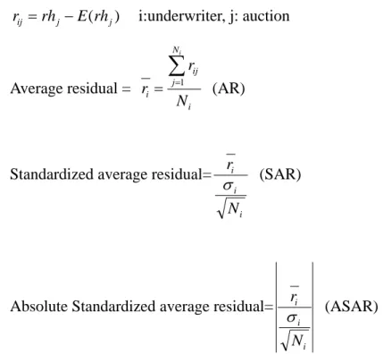
) ( j j ij rh E rh r i:underwriter, j: auction Average residual = i N j ij i N r r i
1 (AR)Standardized average residual=
i i i N r (SAR)
Absolute Standardized average residual=
i i i N r (ASAR)
Table 6 shows each underwriter’s residual. Table 7 further shows that although
residuals for auction have positive and negative numbers, average residuals for
underwriters show only one negative for one underwriter. Underpricing is a
common strategy of underwriters in auction IPOs.
4. Market share
first and in the second sub-period, and calculate the difference.
Market shares are computed by allocating a fraction of on-half or one-third to
each co-manager of an IPO if 2 or 3 co-managed an offering. Marker share
computations are based upon all 41 firms going public during the first and the second
sub-period. We choose underwriters with at least 3 IPOs in the first sub-period.
Market shares are calculated by dividing the net number of IPOs of underwriters
i by the total number of offerings in each sub-period. (41 and 41 in our sample) If an
underwriter had IPOs at the first sub-period, but had no IPOs at the second sub-period,
we still keep this sample, and assign 0 market share at the second sub-period. Table
8 shows mean market share at the first sub-period was 0.019, but the mean market
share for the second sub-period decreased to 0.017. Auction IPOs became less
popular, and issuing firms tended to use fixed-price offerings.
5. OLS results with % change in market share as dependent variable.
(1) Use average residual (AR) as explanatory variable
i i
i AR
mschange 0 1
(2) Use standardized average residual (SAR) as explanatory variable
i i
i SAR
mschange 0 1
(3) Use absolute standardized average residual (ASAR) as explanatory variable
i i
i ASAR
mschange 0 1
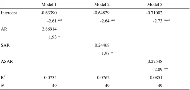
Table 9 shows the relation between market share and residual. At the first glance,
these results are "strange", because they are inconsistent with Beatty and Ritter’s
results. Beatty and Ritter predict that with higher degree of mispricing, market share
will decrease. However, our results show that with higher degree of underpricing,
underwriters will gain more market shares latter. Perhaps, underwriters have no
IPO has higher initial return, they can attract more investors to bid in the next auction
IPO and make it more successful. This behavior can help underwriters to gain more
business latter.
(b) Test Hoberg’s hypothesis following his procedure and variables.
I also try to test Hoberg’s (2007) information hypothesis using auction IPO data.
First, I follow Hoberg’s definition, procedure, and variables to run the tests. Second,
I use the procedure, and variables in Chiang. Qian, and Sherman (2010) to test
Hoberg’s hypothesis. Results show no matter using which model, underwriter
quality defined by Hoberg (2007) can not explain underwriter’s market share.
Underwriters with high previous initial return continue to gain more market share.
3. Frequent Underwriters’ Performance
I first check the performance of frequent leading underwriters.
I use auction order to measure underwriters’ experience. Each
underwriter-auction is assigned an auction order. An auction is an underwriter’s first
(second, third, etc.) auction if the underwriter has 0 (1, 2, etc.) previous IPO auctions.
Thus, auction order is an underwriter’s number of past auctions plus one. A given
auction may be one co-underwriter’s third auction but another co-underwriter’s first
auction. An auction is counted as a previous auction if its first non-hit day occurs
before the current auction’s auction date (so that we can compute the initial return
from the previous auction).
At the first glance, we see the initial return for later auction is smaller than the
previous one. Ex. The average initial return for the 2nd auction order is 0.0743,
smaller than that in the 1st auction order, 0.1721. Similarly, the third auction order is
even smaller at -0.0226. However, when I conduct t-test for the mean difference and
sign rank test for the median difference, I find no significance evidence for the median
difference and for the median difference.
There is no significant evidence for the leading underwriters to have lower initial
return for later auction IPOs. I further check this for co-underwriters. An
underwriter can participate in as many as auction IPOs as they can. I then test the
performance of frequent co-underwriters. The more times underwriters participating
in auction IPOs, the higher average initial return the underwriter have. Underwriters’
IPO returns steadily increase as they participate in more auctions. Figure 5 shows
times of co-underwriter participate in auction IPOs. I want to test:
H0:The more times underwriters participating in auction IPOs, the higher average
initial return the underwriter have.
The dependent variable is the average initial return of underwriters’ auction IPOs.
Table 13 shows there is a trend for higher and higher initial return when underwriters
participate in more auction IPOs. It supports that the more times that underwriters
participate in auction IPOs, the higher average initial return the underwriters will have.
It seems that underwriter will have larger initial return for later auction IPOs when
they gain more experience.
I conclude this section that underwriters did not get less initial return for later
auctions. They should not afraid to have lower later initial return if they attract more
4. Using Underwriters Affiliated Dealers’ Trading to Predict long Run Return
TEJ provides a database for dealer’s trading. The frequency of the data is week. I
use this weekly data of dealers’ trading to trace whether underwriters will use
affiliated dealers’ trade to support an IPO’s long run performance.
I calculate average net buy of the first two weeks after IPOs. I calculate the average
net by for dealers affiliated to the leading underwriters, dealers affiliated to all
co-underwriters, and other dealers. I also have average net buy for all dealers.
I want to test whether this average net buy account can be used to predict an
IPO’s long run returns: 6 months after the 20th trading day, 1-yaer after the 20th trading
day, and 2-year after the 20th trading day.
Results are show on Table 16. Results show that there is no significant impact
of average net-buy on an IPO’s long run return. This implies that underwriters did
not use affiliated dealers’ trading to support an IPO’s long run return.
An underwriter in an auction IPO cares only about large underpricing, and then
the IPO is easier to be successful. Once the IPO is successful, underwriters have no
obligation or incentive to support an IPO’s long run return, because this will not affect
the underwriter’s market share.
5. Conclusions and Suggestions
In this paper, I test three hypotheses to investigate whether underwriters in auction
IPOs care about IPO performance or not. Since underwriters in auction IPOs have
no discretion or pricing ability, I conjecture that underwriters have no incentive to
stabilize IPO performance. They care only about selling out shares, and they do not
care large underpricing.
share and IPO underpricing is positive. This implies that underwriters will lower
offering price (the reserved price in auction IPOs) to attract more individual investors.
With more individual investors, the more likely the IPO will be successful.
The second result is that underwriters’ later IPO case does not necessary get
lower initial return. If underwriters’ later IPO gets lower initial return, it means that
the positive relationship between market share and underpricing can not last long.
Our results support that the relationship between market share and underpricing will
hold for later IPOs. This supports that underwriters in auction IPOs will continue to
have large underpricing.
The third test is whether underwriters’ affiliated dealer can trade to affect an
IPO’s long run return. My result shows this not the case. Underwriter, either the
leading underwriter, or co-underwriters, did not use affiliated dealer’s trade to affect
IPO’s long run return. This evidence again support that underwriters in auction IPOs
will not support an IPO’s performance.
After 2003, there was only on auction IPOs in 2008. Auction IPO is dying.
Currently, in Taiwan, most IPOs are using -. Based on our results, I argue that
underwriters in auction IPOs do not care about the performance of IPOs. They care
only about how to sell shares out. With higher initial return, they get no punishment
from issuing firms, but they can attract more individual investors to participate and
make the IPO be more likely to be successful. Therefore, there is a need to compare
the results in this paper with those for book-building IPOs. I conjecture that, in
References
Beatty, Randolph, and Jay Ritter, 1986, Investment banking, reputation and the underpricing of initial public offerings, Journal of Financial Economics 15, 213–232.
Beatty, Randolph, and Ivo Welch, 1996, Issuer expenses and legal liability in initial public offerings, Journal of Law and Economics 39, 545–602.
Benveniste, Lawrence, Walid Busaba, and William Wilhelm, 2002, Information externalities and the role of underwriters in primary equity markets, Journal of
Financial Intermediation 11, 61–86.
Booth, Lena Chua, 2004, “Underwriter Reputation and Aftermarket Performance of Closed-End Funds,” Journal of Financial Research, 24 (4), pp. 539–557.
Carhart, Mark M., 1997, “On Persistence in Mutual Fund Performance,” Journal of
Finance 52, 57-82.
Yao-Min Chiang, David Hirshleifer, Yiming Qian, Ann Sherman, 2011, “Do Investors Learn from Experience: Evidence from Frequent IPO Investors.” Review of
Financial Studies, Vol. 24 Issue 5, p1560-1589.
Yao-Min Chiang;Yiming Qian;Ann E. Sherman, 2010, "Endogenous entry and partial adjustment in IPO auctions: Are institutional investors better informed?," Review of
Financial Studies, Vol. 23 Issue 3, p1200-1230.
Dunbar, Craig, 2000, Factors affecting investment bank initial public offering market share, Journal of Financial Economics 55, 3–41.
Hoberg, G. “The Underwriter Persistence Phenomenon.” Journal of Finance, 62 (2007), 1169–1206.
Logue, Dennis, Richard Rogalski, James Seward, and Lynn Foster-Johnson, 2002, What’s special about the role of underwriter reputation and market activities in IPOs,
Journal of Business 75, 213–243.
Loughran, Tim, and Jay Ritter, 2002, Why don’t issuers get upset about leaving money on the table in IPOs? Review of Financial Studies 15, 413–433.
Purnanandam, Amiyatosh, and Bhaskaran Swaminathan, 2004, Are IPOs really underpriced? Review of Financial Studies 17, 811–848.
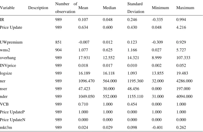
Table 1 Summary statistics
Variable Description Number of
observation Mean Median Standard
Deviation Minimum Maximum
IR 989 0.107 0.048 0.246 -0.335 0.994 Price Update 989 0.634 0.600 0.430 0.048 4.216 UWpremium 851 -0.007 0.012 0.123 -0.309 0.929 wms2 904 1.077 0.625 1.166 0.027 5.727 overhang 989 17.931 12.552 14.321 8.999 107.333 INVprice 989 0.018 0.017 0.010 0.002 0.052 logsize 989 16.189 16.118 1.093 13.855 19.483 ner 989 1096.470 564.000 1195.360 32.000 4286.000 nser 989 47.423 30.000 48.456 0.000 197.000 nder 989 1049.050 552.000 1155.110 31.000 4094.000 VCB 989 0.710 1.000 0.454 0.000 1.000 Price UpdateP 989 1.000 1.000 0.000 1.000 1.000 Price UpdateN 989 0.000 0.000 0.000 0.000 0.000 mkt3m 989 0.024 0.029 0.098 -0.401 0.262
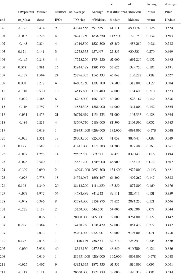
Table 2 Underwriter characteristics und UWpremiu m_Mean Market share Number of IPOs Average IPO size Average # of bidders Average # of institutional bidders Average # of individual bidders Average initial return Average Price Update 74 -0.122 0.474 9 42948.556 891.889 41.111 850.778 0.126 0.524 101 -0.093 0.223 4 78741.750 1836.250 115.500 1720.750 0.134 0.503 102 -0.145 0.234 4 15010.500 1523.500 65.250 1458.250 -0.021 0.783 103 0.121 0.141 3 12273.333 957.667 27.333 930.333 0.270 0.469 104 -0.165 0.218 4 17723.250 1754.250 62.000 1692.250 0.152 0.493 105 0.068 0.891 16 32844.438 1395.375 55.625 1339.750 0.185 0.491 107 -0.107 1.504 24 25296.833 1145.333 45.042 1100.292 0.082 0.627 109 0.000 0.217 4 84807.750 1392.500 74.500 1318.000 0.029 0.304 110 -0.118 0.530 10 14515.800 1171.400 37.000 1134.400 0.210 0.573 112 -0.002 0.485 6 16262.000 1563.667 40.500 1523.167 0.149 0.556 115 -0.116 0.797 13 15835.308 1388.000 44.000 1344.000 0.152 0.564 116 -0.031 1.473 21 26770.619 1154.333 51.000 1103.333 0.128 0.694 118 -0.186 0.233 4 85799.750 2186.000 81.500 2104.500 0.002 0.463 119 0.019 1 289431.000 4286.000 192.000 4094.000 -0.078 0.048 120 -0.035 1.351 17 28703.706 925.000 41.059 883.941 0.087 0.549 121 0.125 0.582 10 41841.000 1120.100 41.700 1078.400 0.163 0.561 122 -0.007 1.295 14 29632.500 869.571 37.429 832.143 0.016 0.494 123 -0.078 0.549 10 15631.200 1209.000 46.900 1162.100 0.072 0.607 124 -0.309 0.090 2 147983.000 2653.500 131.500 2522.000 -0.123 0.621 125 -0.028 0.778 15 34378.067 1556.467 64.200 1492.267 0.147 0.533 126 0.108 1.240 20 28618.200 1116.350 43.550 1072.800 0.160 0.476 127 -0.007 5.977 54 14588.889 841.722 39.111 802.611 0.101 0.759 128 -0.048 0.366 8 52784.000 2159.875 75.625 2084.250 0.121 0.606 131 -0.228 0.119 2 13150.000 546.500 54.000 492.500 0.077 0.344 134 0.036 1 20000.000 905.000 79.000 826.000 0.122 0.142 137 0.285 0.384 7 14430.286 1108.429 57.000 1051.429 0.272 0.437 139 0.033 1 25204.000 972.000 53.000 919.000 0.071 0.760 140 0.197 0.613 7 11136.429 758.571 32.714 725.857 0.205 0.626 207 -0.030 2.936 40 18542.150 957.350 46.650 910.700 0.124 0.626 208 0.019 1 289431.000 4286.000 192.000 4094.000 -0.078 0.048 211 -0.025 0.407 9 45828.333 1872.333 62.333 1810.000 0.093 0.601 212 -0.113 0.111 3 20460.000 1523.333 43.000 1480.333 0.084 0.634
218 -0.092 0.730 14 35293.857 1349.143 50.857 1298.286 0.131 0.460 219 0.126 0.619 10 15272.400 1107.400 43.200 1064.200 0.214 0.498 501 0.083 1 4719.000 410.000 18.000 392.000 -0.100 0.661 508 -0.070 0.630 8 14160.625 1038.125 35.375 1002.750 0.070 0.574 509 0.012 0.932 8 6605.625 421.875 23.750 398.125 -0.025 0.716 511 -0.034 0.630 10 40461.000 1562.700 57.700 1505.000 0.078 0.659 515 -0.011 2.456 29 20997.069 907.379 41.966 865.414 0.156 0.541 518 -0.037 0.187 5 72983.800 2241.400 74.000 2167.400 0.149 0.526 523 0.001 5.035 43 15337.814 894.233 39.442 854.791 0.126 0.728 526 0.090 0.291 4 78590.000 1333.250 65.750 1267.500 0.064 0.408 527 -0.012 3.006 31 20607.839 996.419 46.742 949.677 0.118 0.586 528 -0.261 0.358 5 15395.600 1154.000 37.400 1116.600 -0.018 0.755 529 0.059 3.201 28 10596.714 889.321 31.964 857.357 0.123 0.681 538 0.217 1.324 12 6628.833 543.500 37.833 505.667 0.148 0.853 550 0.019 1 289431.000 4286.000 192.000 4094.000 -0.078 0.048 551 0.041 1.975 24 23427.250 1008.542 51.500 957.042 0.128 0.658 555 0.063 4.282 42 17303.000 938.548 46.952 891.595 0.113 0.796 556 0.125 1 6182.000 1199.000 82.000 1117.000 -0.097 2.362 558 -0.201 0.167 4 83465.500 1595.250 65.500 1529.750 0.070 0.521 565 -0.048 2.454 23 23516.478 932.043 40.565 891.478 0.106 0.624 572 0.000 5.541 49 14795.735 904.224 40.592 863.633 0.057 0.759 582 0.052 2.335 25 22974.000 945.840 40.040 905.800 0.115 0.595 585 -0.051 3.530 34 19475.588 962.147 39.176 922.971 0.086 0.709 592 -0.036 2.893 28 21345.643 1081.893 42.607 1039.286 0.153 0.641 616 0.019 1 289431.000 4286.000 192.000 4094.000 -0.078 0.048 629 -0.054 0.234 2 5592.500 229.500 10.000 219.500 -0.094 0.311 634 0.114 1.436 18 25690.222 813.222 52.722 760.500 0.099 0.574 648 -0.029 0.160 4 84041.500 2599.000 98.250 2500.750 0.057 0.531 653 -0.100 0.671 6 54521.833 1022.333 51.833 970.500 -0.038 0.527 679 0.044 0.300 3 8372.667 353.000 20.667 332.333 0.053 0.599 691 0.019 1 289431.000 4286.000 192.000 4094.000 -0.078 0.048 700 -0.047 0.371 4 81979.000 1336.000 66.000 1270.000 -0.006 0.445 703 -0.066 0.726 8 44598.625 931.250 41.500 889.750 0.021 0.580 718 -0.079 0.144 2 146465.500 2442.000 104.000 2338.000 -0.132 0.783 737 -0.093 0.435 5 8636.000 734.400 47.600 686.800 0.142 1.003 739 -0.033 0.262 3 7324.000 499.667 37.667 462.000 -0.055 0.505 779 0.129 0.379 7 56194.857 1368.857 51.571 1317.286 0.211 0.289 841 -0.120 1.293 15 30381.933 1074.067 43.933 1030.133 0.025 0.648
842 -0.028 0.262 3 13563.333 297.333 22.333 275.000 0.007 0.406 844 0.021 0.662 7 8270.571 790.571 46.143 744.429 0.162 0.454 845 0.017 1.205 17 29297.706 1476.647 54.294 1422.353 0.052 0.732 861 0.019 1 289431.000 4286.000 192.000 4094.000 -0.078 0.048 862 -0.287 0.215 3 100315.333 1812.333 88.000 1724.333 -0.129 0.630 864 0.091 1 8735.000 391.000 19.000 372.000 -0.010 0.557 869 0.592 0.325 2 4043.500 905.000 64.000 841.000 0.288 2.474 870 -0.151 0.210 2 10301.500 605.500 37.500 568.000 -0.047 0.796 873 -0.127 0.609 7 47474.286 1153.571 59.714 1093.857 -0.070 0.733 874 -0.067 0.278 4 80903.250 1765.250 97.750 1667.500 -0.020 0.931 876 0.067 1 10870.000 639.000 29.000 610.000 0.085 0.908 889 -0.030 1.887 25 22431.480 1262.320 48.720 1213.600 0.153 0.690 930 0.126 0.400 8 52950.875 1738.000 64.250 1673.750 0.227 0.466 997 0.015 0.100 2 16430.000 1511.000 65.000 1446.000 0.046 0.778 999 0.038 4.096 44 16923.136 969.136 44.932 924.205 0.120 0.615
Table 3 Use sample in the second sub-period to estimate a return regression.
I follow Chiang, Qian, and Sherman (2010) to estimate entry regression for samples in the second sub-period to estimate unexpected entry of institutions and unexpected entry of individuals. The dependent variable is the log of number of bidder.
Panel A, Institutional bidders.
Parameter Estimate Error t Value Pr > |t|
Intercept -2.36286 2.447066 -0.97 0.3401 logasset 0.57549 0.145687 3.95 0.0003 VC 0.795086 1.706473 0.47 0.6438 PE -0.00545 0.0069 -0.79 0.4342 industry 1.258939 0.472887 2.66 0.0111 excotc 0.283307 0.374103 0.76 0.4533 relativesize 0.426354 7.40659 0.06 0.9544 p3mrmv -32.0544 87.93033 -0.36 0.7174 prevrh 1.881736 1.339076 1.41 0.1677
Panel B, Individual bidders
Parameter Estimate Error t Value Pr > |t|
Intercept 2.376952 1.76785 1.34 0.1863 logasset 0.42757 0.100031 4.27 0.0001 VC 0.414195 0.954564 0.43 0.6667 PE 0.003765 0.00539 0.7 0.4889 industry 0.788395 0.382774 2.06 0.046 excotc 0.452096 0.354611 1.27 0.2097 relativesize 1.486886 5.10147 0.29 0.7722 p3mrmv -73.132 65.40282 -1.12 0.2702 prevrh 2.069488 0.824463 2.51 0.0162
Table 4, Return regression for the second period
This table shows the results of plugging in unexpected entry of institutions and unexpected entry of individuals, premiums, and other variables to run return regression for the second sub-period.
Parameter Estimate Error t Value Pr > |t|
Intercept 0.230078 0.590841 0.39 0.6991 logasset 0.018927 0.039383 0.48 0.6335 VC -0.247 0.245752 -1.01 0.3211 PE -0.00211 0.001633 -1.29 0.2048 industry 0.110226 0.096368 1.14 0.2597 excotc -0.08417 0.108755 -0.77 0.4436 relativesize 0.460528 1.677465 0.27 0.7851 p3mrmv -19.8367 21.02999 -0.94 0.3514 res5 0.137073 0.054074 2.53 0.0154 premins -0.31093 0.423698 -0.73 0.4674 res6 0.0041 0.090862 0.05 0.9642 premind 0.29086 0.477671 0.61 0.5461 prevrh -0.09745 0.539218 -0.18 0.8575
Table 5, Absolute Standardized Average Residual
For samples in the first sub-period, we follow Beatty and Ritter (1986) to measure mispricing by using the “absolute standardized average residual”. I also try “average residual” and “standardized average residual”. n ID rh E(rh) residual 3 8502 0.255687823 -0.05443491 0.310122737 4 8503 0.993796753 0.04192839 0.951868363 5 8504 0.387296638 -0.27079776 0.6580944 6 8505 0.180735901 0.091019125 0.089716776 7 8506 0.219981096 -0.03820225 0.258183342 8 8507 0.478787582 0.276028134 0.202759447 9 8508 0.122123555 0.191258898 -0.06913534 10 8509 0.172705613 0.09449569 0.078209923 11 8510 0.237533581 0.041342354 0.196191227 12 8511 0.632672037 0.281917263 0.350754775 13 8601 0.02144481 0.166306223 -0.14486141 14 8602 0.17627187 0.043982147 0.132289723 15 8603 -0.13963645 0.011512999 -0.15114945 16 8604 -0.1057943 0.189412821 -0.29520712 17 8605 0.041304601 -0.56857317 0.609877776 18 8606 0.045549498 -0.21388107 0.25943057 19 8607 0.28588115 0.074097537 0.211783613 20 8608 0.291888731 0.116979206 0.174909525 21 8609 0.071298962 0.012899051 0.058399911 22 8610 -0.04167708 -0.0382825 -0.00339458 23 8611 -0.27374437 -0.0379072 -0.23583716 24 8612 0.026683937 0.098481061 -0.07179712 25 8613 0.014578363 -0.04486305 0.059441418 26 8614 0.03268163 -0.04413264 0.076814266 27 8615 -0.27349047 0.066294863 -0.33978533 28 8616 -0.09962174 0.009444962 -0.10906671 29 8617 -0.11318703 0.012643804 -0.12583083 30 8618 0.049017729 0.026502289 0.02251544 31 8619 0.12643572 -0.02107398 0.147509701 32 8701 0.939091472 0.078866322 0.86022515 33 8702 0.014677115 -0.03201124 0.046688356
34 8703 0.068101506 -0.03498951 0.103091011 35 8704 -0.10330986 0.042351622 -0.14566148 36 8705 0.028408706 0.038754946 -0.01034624 37 8706 0.038670247 -0.02081601 0.059486257 38 8707 -0.15247395 0.12684898 -0.27932293 39 8708 -0.15600791 0.254327974 -0.41033588 40 8709 0.00992738 -0.12552129 0.13544867 41 8710 0.132764345 -0.14719168 0.279956022 42 8711 -0.01001408 -0.01276366 0.002749581 43 8712 0.010732668 0.230444414 -0.21971175 Average 0.090855479 Median 0.059486257 Stddev 0.293957 Min -0.41034 Max 0.951868
Table 6, Underwriter’s Residual underwriters No of auctions Residual Mean Residual StdDev Residual Min Residual Max 74 7 0.160776 0.333598 -0.12583 0.860225 101 1 0.07821 0.07821 0.07821 102 2 -0.00967 0.140561 -0.10907 0.089717 103 2 0.416502 0.341663 0.17491 0.658094 104 4 0.074643 0.131135 -0.06914 0.196191 105 12 0.210005 0.305576 -0.12583 0.951868 107 19 0.078336 0.244172 -0.33979 0.860225 109 2 0.163322 0.164945 0.046688 0.279956 110 9 0.21062 0.319618 -0.12583 0.951868 112 5 0.197929 0.292271 -0.14486 0.658094 115 12 0.116833 0.113616 -0.12583 0.310123 116 12 0.146059 0.351142 -0.27932 0.951868 118 1 0.089717 0.089717 0.089717 120 14 0.090926 0.249608 -0.14566 0.860225 121 7 0.231456 0.329659 -0.00339 0.951868 122 8 0.068452 0.127902 -0.10907 0.310123 123 10 0.02653 0.168759 -0.33979 0.211784 125 10 0.135263 0.342232 -0.33979 0.951868 126 14 0.222586 0.354987 -0.14486 0.951868 127 29 0.134262 0.310782 -0.33979 0.951868 128 6 0.128888 0.076075 0.022515 0.211784 131 2 0.003839 0.103202 -0.06914 0.076814 134 1 -0.06914 -0.06914 -0.06914 137 7 0.192306 0.352645 -0.0718 0.951868 139 1 0.0584 0.0584 0.0584 140 7 0.12872 0.383496 -0.41034 0.860225 207 26 0.149269 0.284881 -0.21971 0.951868 211 8 0.095421 0.215702 -0.33979 0.310123 212 3 0.09245 0.165631 -0.0718 0.259431 218 11 0.135681 0.385642 -0.33979 0.951868 219 7 0.156782 0.397253 -0.27932 0.951868 501 1 -0.10907 -0.10907 -0.10907 508 6 0.061189 0.133574 -0.0718 0.310123 509 1 0.14751 0.14751 0.14751
511 8 0.085355 0.160873 -0.14486 0.259431 515 15 0.289268 0.306955 -0.06914 0.951868 518 3 0.17427 0.084235 0.089717 0.258183 523 19 0.138249 0.332574 -0.33979 0.951868 527 17 0.117183 0.291615 -0.41034 0.951868 528 3 -0.07175 0.162793 -0.23584 0.089717 529 19 0.11398 0.308946 -0.29521 0.951868 538 4 0.1942 0.452363 -0.14566 0.860225 551 11 0.222657 0.315566 -0.10907 0.951868 555 25 0.100136 0.281537 -0.33979 0.951868 558 2 0.158292 0.141268 0.0584 0.258183 565 9 0.165433 0.201675 0.00275 0.658094 572 25 0.033998 0.285444 -0.41034 0.951868 582 16 0.228964 0.319041 -0.14566 0.951868 585 19 0.163919 0.27421 -0.33979 0.951868 592 18 0.212415 0.297079 -0.23584 0.951868 629 1 0.00275 0.00275 0.00275 634 10 0.097581 0.296057 -0.21971 0.860225 648 3 0.103587 0.217473 -0.14486 0.259431 653 2 -0.00511 0.198775 -0.14566 0.135449 679 1 0.022515 0.022515 0.022515 700 1 0.046688 0.046688 0.046688 703 6 0.075466 0.35556 -0.29521 0.658094 739 1 0.135449 0.135449 0.135449 779 6 0.291167 0.446564 -0.27932 0.951868 841 10 0.021516 0.184322 -0.33979 0.259431 842 1 0.046688 0.046688 0.046688 844 3 0.416058 0.210152 0.279956 0.658094 845 13 0.064526 0.176723 -0.33979 0.259431 864 1 0.00275 0.00275 0.00275 870 2 -0.00511 0.198775 -0.14566 0.135449 873 1 -0.27932 -0.27932 -0.27932 889 17 0.12966 0.306601 -0.33979 0.951868 930 6 0.223008 0.366604 -0.06914 0.951868 997 2 -0.04323 0.143727 -0.14486 0.0584 999 26 0.130255 0.315807 -0.41034 0.951868
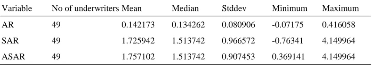
Table 7 Residual in the First Period
This table shows “absolute standardized average residual”, “average residual”, and “standardized average residual” for the underwriters in the first sub-period.
Variable No of underwriters Mean Median Stddev Minimum Maximum AR 49 0.142173 0.134262 0.080906 -0.07175 0.416058 SAR 49 1.725942 1.513742 0.966572 -0.76341 4.149964 ASAR 49 1.757102 1.513742 0.907453 0.369141 4.149964
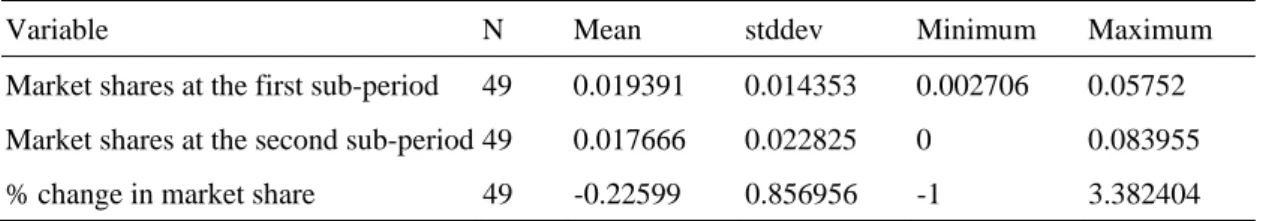
Table 8 Market share
We follow Beatty and Ritter (1986) to calculate market shares of underwriters in the first and in the second sub-period, and calculate the difference.
Variable N Mean stddev Minimum Maximum
Market shares at the first sub-period 49 0.019391 0.014353 0.002706 0.05752 Market shares at the second sub-period 49 0.017666 0.022825 0 0.083955 % change in market share 49 -0.22599 0.856956 -1 3.382404
Table 9 Regression with % change in market share as dependent variable.
Model 1: Use average residual (AR) as explanatory variable:
i i
i AR
mschange 0 1
Model 2: Use standardized average residual (SAR) as explanatory variable
i i
i SAR
mschange 0 1
Model 3: Use absolute standardized average residual (ASAR) as explanatory variable
Model 1 Model 2 Model 3
Intercept -0.63390 -0.64829 -0.71002 -2.61 ** -2.64 ** -2.73 *** AR 2.86914 1.93 * SAR 0.24468 1.97 * ASAR 0.27548 2.09 ** R2 0.0734 0.0762 0.0851 N 49 49 49 i i i ASAR mschange 01
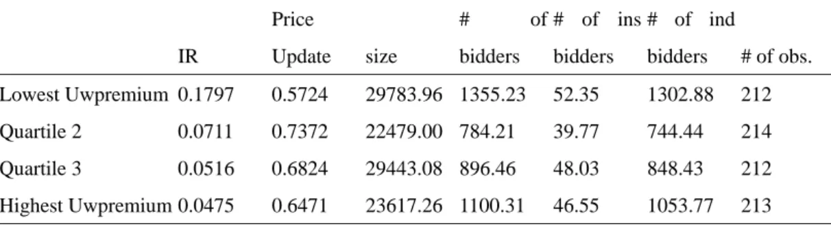
Table 10 IPO characteristics versus underwriter quality quartile
I follow Hoberg to run regression: variable=b1*logsize+b2*logsize^2+b3*industry+e. Then calculate residual, average residual for each quartile.
Panel A, IR Price Update size # of bidders # of ins bidders # of ind bidders # of obs. Lowest Uwpremium 0.1797 0.5724 29783.96 1355.23 52.35 1302.88 212 Quartile 2 0.0711 0.7372 22479.00 784.21 39.77 744.44 214 Quartile 3 0.0516 0.6824 29443.08 896.46 48.03 848.43 212 Highest Uwpremium 0.0475 0.6471 23617.26 1100.31 46.55 1053.77 213 Panel B, IR Price Update size # of bidders # of ins bidders # of ind bidders # of obs. Lowest Market share 0.1988 0.5521 26809.69 1541.07 54.87 1486.19 226 Quartile 2 0.1032 0.6176 26242.49 1144.53 46.25 1098.28 226 Quartile 3 0.0475 0.6525 26236.58 858.00 42.70 815.29 226 Highest Market share 0.0428 0.7728 24459.61 768.15 45.66 722.48 226
Panel C, Residual IR, Price Update, from the regression as Hoberg’s model.
IR Price Update # of obs.
Lowest Uwpremium 0.0643 -0.0025 212
Quartile 2 -0.0274 0.0491 214
Quartile 3 -0.0481 0.0108 212
Highest Uwpremium -0.0576 -0.0165 213
Panel D,
IR Price Update # of obs.
Lowest Market share 0.0857 -0.0101 226
Quartile 2 -0.0155 0.0096 226
Quartile 3 -0.0566 0.0008 226
Figure 1 Underwriter 999, 44 IPOs. Average UWpremium= 0.02770. IR>median: 45.45%, IR<median: 54.55%. Price Update>median: 52.27%, Price Update<median: 47.73%
Figure 2, Underwriter 127, 54 IPOs. Average UWpremium=-0.01274. IR>median: 55.56%, IR<median: 44.44%. Price Update>median: 42.59%, Price Update<median: 57.41%.
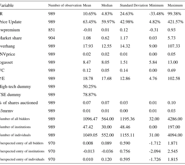
Table 11 Test Hoberg’s hypothesis following Chiang, Qian and Sherman (2009, RFS) procedure and variables.
Panel A, Summary statistics
Variable Number of observation Mean Median Standard Deviation Minimum Maximum
IR 989 10.65% 4.83% 24.63% -33.48% 99.38% Price Update 989 63.45% 59.97% 42.98% 4.82% 421.57% uwpremium 851 -0.01 0.01 0.12 -0.31 0.93 Market share 904 1.08 0.62 1.17 0.03 5.73 overhang 989 17.93 12.55 14.32 9.00 107.33 INVprice 989 0.02 0.02 0.01 0.00 0.05 logasset 989 8.47 8.05 1.51 5.84 13.00 VC 989 0.12 0.05 0.14 0.00 0.69 P/E 989 18.78 17.68 12.86 4.76 102.58 High-tech dummy 989 50.25% TSE dummy 989 78.87% % of shares auctioned 989 0.07 0.07 0.03 0.01 0.10 p3mrmv 989 0.01 0.01 0.00 0.01 0.03
Number of all bidders 989 1096.47 564.00 1195.36 32.00 4286.00 Number of institutions 989 47.42 30.00 48.46 0.00 197.00 Number of individuals 989 1049.05 552.00 1155.11 31.00 4094.00 Unexpected entry of all bidders 970 0.008 0.089 0.590 -1.712 1.871 Unexpected entry of institutions 970 -0.013 -0.036 0.756 -2.094 2.545 Unexpected entry of individuals 970 0.010 0.120 0.595 -1.726 1.815
Panel B, Underwriter characteristics und UWpremiu m_Mean Market share Number of IPOs Average IPO size Average # of bidders Average # of institutional bidders Average # of individual bidders Average initial return Average Price Update 74 -0.122 0.474 9 42948.556 891.889 41.111 850.778 0.126 0.524 101 -0.093 0.223 4 78741.750 1836.250 115.500 1720.750 0.134 0.503 102 -0.145 0.234 4 15010.500 1523.500 65.250 1458.250 -0.021 0.783 103 0.121 0.141 3 12273.333 957.667 27.333 930.333 0.270 0.469 104 -0.165 0.218 4 17723.250 1754.250 62.000 1692.250 0.152 0.493 105 0.068 0.891 16 32844.438 1395.375 55.625 1339.750 0.185 0.491 107 -0.107 1.504 24 25296.833 1145.333 45.042 1100.292 0.082 0.627 109 0.000 0.217 4 84807.750 1392.500 74.500 1318.000 0.029 0.304 110 -0.118 0.530 10 14515.800 1171.400 37.000 1134.400 0.210 0.573 112 -0.002 0.485 6 16262.000 1563.667 40.500 1523.167 0.149 0.556 115 -0.116 0.797 13 15835.308 1388.000 44.000 1344.000 0.152 0.564 116 -0.031 1.473 21 26770.619 1154.333 51.000 1103.333 0.128 0.694 118 -0.186 0.233 4 85799.750 2186.000 81.500 2104.500 0.002 0.463 119 0.019 1 289431.000 4286.000 192.000 4094.000 -0.078 0.048 120 -0.035 1.351 17 28703.706 925.000 41.059 883.941 0.087 0.549 121 0.125 0.582 10 41841.000 1120.100 41.700 1078.400 0.163 0.561 122 -0.007 1.295 14 29632.500 869.571 37.429 832.143 0.016 0.494 123 -0.078 0.549 10 15631.200 1209.000 46.900 1162.100 0.072 0.607 124 -0.309 0.090 2 147983.000 2653.500 131.500 2522.000 -0.123 0.621 125 -0.028 0.778 15 34378.067 1556.467 64.200 1492.267 0.147 0.533 126 0.108 1.240 20 28618.200 1116.350 43.550 1072.800 0.160 0.476 127 -0.007 5.977 54 14588.889 841.722 39.111 802.611 0.101 0.759 128 -0.048 0.366 8 52784.000 2159.875 75.625 2084.250 0.121 0.606 131 -0.228 0.119 2 13150.000 546.500 54.000 492.500 0.077 0.344 134 0.036 1 20000.000 905.000 79.000 826.000 0.122 0.142 137 0.285 0.384 7 14430.286 1108.429 57.000 1051.429 0.272 0.437 139 0.033 1 25204.000 972.000 53.000 919.000 0.071 0.760 140 0.197 0.613 7 11136.429 758.571 32.714 725.857 0.205 0.626 207 -0.030 2.936 40 18542.150 957.350 46.650 910.700 0.124 0.626 208 0.019 1 289431.000 4286.000 192.000 4094.000 -0.078 0.048 211 -0.025 0.407 9 45828.333 1872.333 62.333 1810.000 0.093 0.601 212 -0.113 0.111 3 20460.000 1523.333 43.000 1480.333 0.084 0.634 218 -0.092 0.730 14 35293.857 1349.143 50.857 1298.286 0.131 0.460
219 0.126 0.619 10 15272.400 1107.400 43.200 1064.200 0.214 0.498 501 0.083 1 4719.000 410.000 18.000 392.000 -0.100 0.661 508 -0.070 0.630 8 14160.625 1038.125 35.375 1002.750 0.070 0.574 509 0.012 0.932 8 6605.625 421.875 23.750 398.125 -0.025 0.716 511 -0.034 0.630 10 40461.000 1562.700 57.700 1505.000 0.078 0.659 515 -0.011 2.456 29 20997.069 907.379 41.966 865.414 0.156 0.541 518 -0.037 0.187 5 72983.800 2241.400 74.000 2167.400 0.149 0.526 523 0.001 5.035 43 15337.814 894.233 39.442 854.791 0.126 0.728 526 0.090 0.291 4 78590.000 1333.250 65.750 1267.500 0.064 0.408 527 -0.012 3.006 31 20607.839 996.419 46.742 949.677 0.118 0.586 528 -0.261 0.358 5 15395.600 1154.000 37.400 1116.600 -0.018 0.755 529 0.059 3.201 28 10596.714 889.321 31.964 857.357 0.123 0.681 538 0.217 1.324 12 6628.833 543.500 37.833 505.667 0.148 0.853 550 0.019 1 289431.000 4286.000 192.000 4094.000 -0.078 0.048 551 0.041 1.975 24 23427.250 1008.542 51.500 957.042 0.128 0.658 555 0.063 4.282 42 17303.000 938.548 46.952 891.595 0.113 0.796 556 0.125 1 6182.000 1199.000 82.000 1117.000 -0.097 2.362 558 -0.201 0.167 4 83465.500 1595.250 65.500 1529.750 0.070 0.521 565 -0.048 2.454 23 23516.478 932.043 40.565 891.478 0.106 0.624 572 0.000 5.541 49 14795.735 904.224 40.592 863.633 0.057 0.759 582 0.052 2.335 25 22974.000 945.840 40.040 905.800 0.115 0.595 585 -0.051 3.530 34 19475.588 962.147 39.176 922.971 0.086 0.709 592 -0.036 2.893 28 21345.643 1081.893 42.607 1039.286 0.153 0.641 616 0.019 1 289431.000 4286.000 192.000 4094.000 -0.078 0.048 629 -0.054 0.234 2 5592.500 229.500 10.000 219.500 -0.094 0.311 634 0.114 1.436 18 25690.222 813.222 52.722 760.500 0.099 0.574 648 -0.029 0.160 4 84041.500 2599.000 98.250 2500.750 0.057 0.531 653 -0.100 0.671 6 54521.833 1022.333 51.833 970.500 -0.038 0.527 679 0.044 0.300 3 8372.667 353.000 20.667 332.333 0.053 0.599 691 0.019 1 289431.000 4286.000 192.000 4094.000 -0.078 0.048 700 -0.047 0.371 4 81979.000 1336.000 66.000 1270.000 -0.006 0.445 703 -0.066 0.726 8 44598.625 931.250 41.500 889.750 0.021 0.580 718 -0.079 0.144 2 146465.500 2442.000 104.000 2338.000 -0.132 0.783 737 -0.093 0.435 5 8636.000 734.400 47.600 686.800 0.142 1.003 739 -0.033 0.262 3 7324.000 499.667 37.667 462.000 -0.055 0.505 779 0.129 0.379 7 56194.857 1368.857 51.571 1317.286 0.211 0.289 841 -0.120 1.293 15 30381.933 1074.067 43.933 1030.133 0.025 0.648 842 -0.028 0.262 3 13563.333 297.333 22.333 275.000 0.007 0.406
844 0.021 0.662 7 8270.571 790.571 46.143 744.429 0.162 0.454 845 0.017 1.205 17 29297.706 1476.647 54.294 1422.353 0.052 0.732 861 0.019 1 289431.000 4286.000 192.000 4094.000 -0.078 0.048 862 -0.287 0.215 3 100315.333 1812.333 88.000 1724.333 -0.129 0.630 864 0.091 1 8735.000 391.000 19.000 372.000 -0.010 0.557 869 0.592 0.325 2 4043.500 905.000 64.000 841.000 0.288 2.474 870 -0.151 0.210 2 10301.500 605.500 37.500 568.000 -0.047 0.796 873 -0.127 0.609 7 47474.286 1153.571 59.714 1093.857 -0.070 0.733 874 -0.067 0.278 4 80903.250 1765.250 97.750 1667.500 -0.020 0.931 876 0.067 1 10870.000 639.000 29.000 610.000 0.085 0.908 889 -0.030 1.887 25 22431.480 1262.320 48.720 1213.600 0.153 0.690 930 0.126 0.400 8 52950.875 1738.000 64.250 1673.750 0.227 0.466 997 0.015 0.100 2 16430.000 1511.000 65.000 1446.000 0.046 0.778 999 0.038 4.096 44 16923.136 969.136 44.932 924.205 0.120 0.615
Panel C, IPO characteristics versus underwriter quality quartile
I follow Hoberg to run regression: variable=b1*logsize+b2*logsize^2+b3*industry+e. Then calculate residual, average residual for each quartile.
IR Price Update size # of bidders # of ins bidders # of ind
bidders res4 res5 res6 # of obs. Lowest Uwpremium 0.1797 0.5724 29783.96 1355.23 52.35 1302.88 -0.0620 -0.1051 -0.0566 212 Quartile 2 0.0711 0.7372 22479 784.21 39.77 744.44 0.0644 0.0902 0.0632 214 Quartile 3 0.0516 0.6824 29443.08 896.46 48.03 848.43 0.1357 0.1065 0.1359 212 Highest Uwpremium 0.0475 0.6471 23617.26 1100.31 46.55 1053.77 -0.0187 -0.0455 -0.0142 213 IR Price Update size # of bidders # of ins bidders # of ind
bidders res4 res5 res6 # of obs. Lowest Market share 0.1988 0.5521 26809.69 1541.07 54.87 1486.19 -0.08966 -0.13431 -0.08366 226 Quartile 2 0.1032 0.6176 26242.49 1144.53 46.25 1098.28 0.029588 0.011693 0.033073 226 Quartile 3 0.0475 0.6525 26236.58 858 42.7 815.29 0.055095 0.009832 0.055598 226 Highest Market share 0.0428 0.7728 24459.61 768.15 45.66 722.48 0.058251 0.105086 0.056994 226
Panel D, Residual IR, Price Update, from the regression as Hoberg’s model.
IR Price Update # of obs.
Lowest Uwpremium 0.0643 -0.0025 212
Quartile 2 -0.0274 0.0491 214
Quartile 3 -0.0481 0.0108 212
Highest Uwpremium -0.0576 -0.0165 213
IR Price Update # of obs.
Lowest Market share 0.0857 -0.0101 226
Quartile 2 -0.0155 0.0096 226
Quartile 3 -0.0566 0.0008 226
Figure 3
Underwriter 999, 44 IPOs. Average UWpremium= 0.02770 IR>median: 45.45%, IR<median: 54.55%.
Price Update>median: 52.27%, Price Update<median: 47.73%
Figure 4,
Underwriter 127, 54 IPOs. Average UWpremium=-0.01274 IR>median: 55.56%, IR<median: 44.44%. 0.04832
Panel E, using Hoberg’s variables, Y=IR
(1) (2)
Estimates t-value Estimates t-value
Intercept 0.114 (3.22) *** 0.502 (0.96) uwpremium -0.362 (-1.43) -0.359 (-1.41) wms2 -0.025 (-1.70) * -0.026 (-2.26) ** overhang -0.001 (-0.93) logsize -0.015 (-0.49) INVprice -6.161 (-2.21) ** VC -0.184 (-1.11) R2 6.17% 13.36% N 851 851
Panel F, using our variables, Y=IR
(3) (4)
Estimates t-value Estimates t-value
Intercept -1.042 (-2.61) ** -1.325 (-2.77) *** uwpremium -0.091 (-0.87) -0.112 (-1.23) wms2 -0.004 (-0.51) -0.009 (-1.19) logasset 0.046 (2.45) ** 0.064 (2.92) *** VC -0.105 (-0.76) -0.081 (-0.64) PE -0.003 (-2.81) *** -0.004 (-2.82) *** industry 0.176 (3.40) *** 0.210 (4.15) *** excotc -0.169 (-2.29) ** -0.185 (-2.56) ** relatives 2.447 (1.65) 3.029 (2.09) ** p3mrmv 27.511 (1.81) * 30.247 (2.10) ** res5 0.097 (2.67) *** premins 0.525 (2.06) ** res6 -0.125 (-2.36) ** premind -0.478 (-1.94) *
year yes yes
R2 44.51% 54.02%
Panel G, Y=IR, uwPrice UpdateP=high/low uwpremium * Price Update Estimates t-value Intercept -1.371 (-2.80) *** uwpPrice Updatep -0.033 (-2.22) ** logasset 0.065 (2.83) *** VC -0.073 (-0.59) PE -0.004 (-3.07) *** industry 0.225 (4.43) *** excotc -0.193 (-2.70) *** relatives 3.251 (2.28) ** p3mrmv 32.385 (2.34) ** res5 0.091 (2.44) ** premins 0.598 (2.35) ** res6 -0.140 (-2.46) ** premind -0.555 (-2.26) ** year yes R2 59.48% N 962
Panel H, Y=market share Estimates t-value Intercept 2.029 (3.00) *** uwpremium 0.634 (1.92) * logasset -0.120 (-2.99) *** VC 0.261 (1.23) PE 0.003 (0.89) industry 0.187 (2.44) ** excotc -0.199 (-1.73) * relatives -1.842 (-0.90) p3mrmv 46.964 (2.39) ** res5 0.063 (1.01) premins 0.292 (0.76) res6 -0.110 (-1.40) premind 0.102 (0.24) year yes R2 40.69% N 843
Table 12 Leading underwriters’ mean return by auction order
This table shows average return for the leading underwriters who have underwrite 1 IPO, 2 IPOs, 3 IPOs, etc.
Sequence N Mean Median Stddev Minimum Maximum
1 22 0.1721 0.1474 0.2855 -0.1443 0.9938 2 17 0.0743 0.0379 0.2125 -0.2737 0.4788 3 10 -0.0226 -0.0425 0.1572 -0.2134 0.2859 4 9 0.0855 0.0377 0.3380 -0.2735 0.9391 5 7 0.0801 0.0099 0.2686 -0.0826 0.6728 6 7 -0.1583 -0.1560 0.1184 -0.3348 0.0091 7 6 0.0728 0.0477 0.1258 -0.0660 0.2856 8 3 -0.0454 -0.0453 0.0912 -0.1367 0.0457 9 1 0.1300 0.1300 . 0.1300 0.1300 10 2 0.1748 0.1748 0.1934 0.0380 0.3116 11 1 0.0048 0.0048 . 0.0048 0.0048 12 1 -0.0119 -0.0119 . -0.0119 -0.0119 13 1 0.0483 0.0483 . 0.0483 0.0483 14 1 0.0583 0.0583 . 0.0583 0.0583 15 1 -0.1684 -0.1684 . -0.1684 -0.1684 16 1 0.2967 0.2967 . 0.2967 0.2967 17 4 0.0489 0.0496 0.1894 -0.1411 0.2375
Figure 5, Times of co-underwriter participate in auction IPOs. 0 2 4 6 8 10 12 14 1 3 5 7 9 12 14 16 18 21 24 28 31 40 43 49 times
No. of underwriters
No. of underwritersTable 13 Co-underwriter returns by auction order
This table shows an co-underwriter return in each auction. We count each underwriter in an underwriting syndicate. Auction order is defined as follows: an auction is an underwriter’s 1st (2nd, 3rd, etc.) auction if the underwriter has 0 (1, 2, etc) previous IPO auctions.
Auction
order Mean return
1 0.196404 2 0.239249 3 0.238598 4 0.127258 5 0.132616 6 0.184791 7 0.09567 8 0.107275 9 0.038642 10 0.062194 11 0.097118 12 0.036096 13 0.085265 14 0.053482 15 0.025728 16 -0.01548 17 0.018977 18 -0.03454 19 0.117482 20 0.150824 21 0.029685 22 0.000236 23 0.049503 24 0.016473 25 0.09007 26 -0.00606 27 0.052507 28 -0.00486 29 0.093243 30 -0.00118
31 0.060389 32 0.168417 33 -0.10737 34 0.0363 35 0.174175 36 0.090105 37 0.078441 38 0.236921 39 -0.05257 40 -0.11506 41 -0.03997 42 0.04833 43 0.196095 44 0.055969 45 0.243617 46 -0.14846 47 0.189972 48 0.109303 49 -0.18417 50 -0.18554 51 -0.07806 52 -0.08259 53 -0.21338 54 -0.27106
Table 14 Dependent variable: average initial return of underwriters’ auction IPOs
Variable Estimate t-value
Intercept 0.04004 (2.85)***
No of times participating 0.00266 (3.23)***
R2 0.1117
Table 15 IPO long run return predicted by dealers’ trading
This table shows how underwriters’ affiliated dealers trade affect IPOs’ long run return. Averagenetbuye1 is the average net buy of leading underwriter’s affiliated dealer during the first two weeks after IPO. Averagenetbuye2 is the average net buy of co-underwriter’s affiliated dealer during the first two weeks after IPO. Averagenetbuye3 is the average net buy of dealers not affiliated to the leading underwriter or the co-underwriters during the first two weeks after IPO. Averagenetbuye1 is the average net buy of all dealers during the first two weeks after IPO.
Panel A, Dependent variable is 6-month return
Variable Estimate t-value Estimate t-value Estimate t-value Estimate t-value Estimate t-value Estimate t-value Intercept 0.1114 (2.28) ** 0.1109 (2.26) ** 0.1090 (2.16) ** 0.1105 (2.24) ** 0.1067 (2.04) ** 0.1649 (0.36) averagenetbuy1 0.0000 (-0.04) -0.0002 (-0.17) 0.0001 (0.05) averagenetbuy2 0.0001 (0.13) 0.0001 (0.15) 0.0001 (0.08) averagenetbuy3 0.0002 (0.19) 0.0003 (0.24) 0.0009 (0.67) averagenetbuy4 0.0001 (0.14) logasset -0.0511 (-0.77) Debtratio 0.0604 (0.18) relativesize 1391.2932 (0.56) PE 0.0046 (1.08) VC 0.7082 (2.22) ** insider -0.0263 (-0.08) excotc 0.0927 (0.61)
Panel B, Dependent variable is 1-year return
Variable Estimate t-value Estimate t-value Estimate t-value Estimate t-value Estimate t-value Estimate t-value Intercept 0.1498 (2.03) ** 0.1533 (2.07) ** 0.1288 (1.70) * 0.1497 (2.01) ** 0.1137 (1.46) 1.1931 (1.71) * averagenetbuy1 -0.0007 (-0.41) -0.0020 (-1.04) -0.0030 (-1.36) averagenetbuy2 -0.0004 (-0.29) -0.0002 (-0.19) 0.0002 (0.11) averagenetbuy3 0.0019 (1.16) 0.0028 (1.53) 0.0043 (2.05) ** averagenetbuy4 0.0001 (0.17) logasset -0.1610 (-1.60) Debtratio 0.0220 (0.04) relativesize -792.6728 (-0.21) PE 0.0034 (0.52) VC 0.3389 (0.70) insider 0.1882 (0.36) excotc 0.0420 (0.18)
Panel C, Dependent variable is 2-year return
Variable Estimate t-value Estimate t-value Estimate t-value Estimate t-value Estimate t-value Estimate t-value Intercept 0.0014 (0.08) 0.0013 (0.07) 0.0044 (0.24) 0.0023 (0.13) 0.0035 (0.18) 0.0365 (0.21) averagenetbuy1 -0.0001 (-0.34) -0.0001 (-0.14) -0.0001 (-0.23) averagenetbuy2 0.0001 (0.29) 0.0001 (0.35) 0.0002 (0.73) averagenetbuy3 -0.0002 (-0.56) -0.0002 (-0.44) -0.0005 (-0.86) averagenetbuy4 0.0000 (-0.22) logasset -0.0084 (-0.33) Debtratio 0.0698 (0.54) relativesize -1276.540 (-1.35) PE 0.0015 (0.93) VC 0.0498 (0.41) insider 0.0733 (0.55) excotc 0.0420 (0.72)
日期:2011/07/31
國科會補助計畫
計畫名稱: 以競價拍賣新股上市資料驗證新股折價與承銷商市場佔有率關係 計畫主持人: 姜堯民 計畫編號: 99-2410-H-004-065- 學門領域: 財務無研發成果推廣資料
計畫主持人:姜堯民 計畫編號:99-2410-H-004-065- 計畫名稱:以競價拍賣新股上市資料驗證新股折價與承銷商市場佔有率關係 量化 成果項目 實際已達成 數(被接受 或已發表) 預期總達成 數(含實際已 達成數) 本計畫實 際貢獻百 分比 單位 備 註 ( 質 化 說 明:如 數 個 計 畫 共 同 成 果、成 果 列 為 該 期 刊 之 封 面 故 事 ... 等) 期刊論文 0 0 100% 研究報告/技術報告 0 0 100% 研討會論文 0 0 100% 篇 論文著作 專書 0 0 100% 申請中件數 0 0 100% 專利 已獲得件數 0 0 100% 件 件數 0 0 100% 件 技術移轉 權利金 0 0 100% 千元 碩士生 0 0 100% 博士生 0 0 100% 博士後研究員 0 0 100% 國內 參與計畫人力 (本國籍) 專任助理 0 0 100% 人次 期刊論文 0 0 100% 研究報告/技術報告 0 0 100% 研討會論文 0 0 100% 篇 論文著作 專書 0 0 100% 章/本 申請中件數 0 0 100% 專利 已獲得件數 0 0 100% 件 件數 0 0 100% 件 技術移轉 權利金 0 0 100% 千元 碩士生 0 0 100% 博士生 0 0 100% 博士後研究員 0 0 100% 國外 參與計畫人力 (外國籍) 專任助理 0 0 100% 人次