國
立
交
通
大
學
機械工程學系
碩
士
論
文
整數階與分數階變革式心搏系統的渾沌及其同步與
反控制
Chaos, Its Synchronization and Anticontrol of Integral and
Fractional Order Modified Heartbeat Systems
研 究 生: 張安瑞
指導教授: 戈正銘 教授
Fractional Order Modified Heartbeat Systems
研 究 生: 張安瑞 Student:An-Ray Zhang 指導教授: 戈正銘 Advisor:Zheng-Ming Ge國 立 交 通 大 學
機 械 工 程 學 系
碩 士 論 文
A ThesisSubmitted to Department of Mechanical Engineering College of Engineering
National Chiao Tung University In Partial Fulfillment of the Requirements
For the Degree of Master of Science In
Mechanical Engineering June 2006
Hsinchu, Taiwan, Republic of China
整數階與分數階變革式心搏系統的渾沌及其同步與反控制
學生:張安瑞 指導教授:戈正銘
摘
要
本篇論文探討有關整數階與分數階變革式心搏系統的渾沌、渾沌同步及其反控 制。藉由相圖、龐卡萊圖及分歧圖等數值模擬結果,可以得知週期及渾沌的現象。 另外經由參數激發法使得兩個非耦合的整數階或分數階變革式心搏系統達到同步。 並透過外加常數項或非線性項獲得分數階變革式心搏系統的反控制。最後,成功的 利用參數激發的方式,讓整數階與分數階的變革式心搏系統達到渾沌化。
Department of Mechanical Engineering National Chiao Tung University
Abstract
Chaos, chaos synchronization and anticontrol for integral and fractional modified heartbeat systems are studied in the thesis. By applying numerical results, phase portrait, Poincaré maps and bifurcation diagrams, a variety of the phenomena of the periodic and chaotic motion can be presented. The synchronizations of two uncoupled integral and fractional order chaotic modified heartbeat systems are accomplished by parameter excited synchronization. Anticontrol of chaos of fractional order modified heartbeat systems can be obtained by addition of a constant term and addition of a nonlinear term. Chaotization of integral and fractional order modified heartbeat systems by parameter excited method, replacement of the parameter of first system by the function of the chaotic state variables of a second chaotic system, is successfully accomplished.
ACKNOWLEDGMENT
利用兩年的時間完成了本篇論文及碩士學位,其中最感謝的不外乎是給予耐心 指導與教誨的 戈正銘教授。教授不僅傳授在專業領域上的知識,更藉由與教授的 相處,使得學生無論是在看待事物的態度或是在處理事情的方法都有明顯的改變。 此外,教授無論是在專業領域或是文學、史學甚至哲學的博學讓學生深感佩服,並 領會到老師的真智慧。 在研究的兩年當中,感謝學長陳炎生、楊振雄、張晉銘在渾沌方面知識的指導 與程式的應用。尤其感謝張晉銘學長的大力幫忙,使得本篇論文得以更加完善。其 次感謝同學易昌賢與歐展義無論在課業上或是論文研討方面的幫忙,使得學生做起 事來事半功倍,充分展現團結的力量。另外,感謝實驗室其他的成員對學生在各方 面的支持與幫忙,讓學生可以心無旁鶩專心致力於課業與論文的研究。 在二十幾年來的求學過程中,感謝父母及兩位姐姐在生活上給予全力的支持, 雖然在求學過程中有著諸多的崎嶇,但他們都無怨無悔的付出,讓學生可以不必擔 心課業以外的事與物,得以全心衝刺以造就現今的我。最後,感謝忠翰、柏豪、俊 明、佩珊與依萍,謝謝你們分享我的喜怒哀樂,讓我的心情得以宣洩。再一次感謝 大家的幫忙與支持,在此獻上十二萬分的敬意。Chapter 1 Introduction...1
Chapter 2 A Fractional Derivative and a Modified Heartbeat System ...3 2.1 A fractional derivative and its approximation 3 2.2 A modified heartbeat system and the corresponding fractional order system 4
Chapter 3 Chaos in a Modified Heartbeat System and in Its Fractional order
Systems...6 3.1 Chaos in a integral order modified heartbeat system 6 3.2 Chaos in a fractional order modified heartbeat system 6
Chapter 4 Parameter Excited Chaos Synchronizations of Integral and Fractional Order Modified Heartbeat Systems ...39 4.1 The scheme of parameter excited chaos synchronizations 39 4.2 Parameter Excited Chaos Synchronization by kcosx、kcosy、kcosxcosy 40
4.2.1 Parameter Excited Chaos Synchronizations by kcosx 40 4.2.2 Parameter Excited Chaos Synchronizations by kcosy 41 4.2.3 Parameter Excited Chaos Synchronizations by kcosxcosy 41
Chapter 5 Anticontrol of Chaos of the Fractional Order Modified Heartbeat
Systems...73 5.1 Anticontrol of Chaos by addition of a constant term 73 5.2 Anticontrol of Chaos by addition of a nonlinear term 74
Chapter 6 Parameter Excited Chaotization of Integral and Fractional Order
6.1 A nano resonator system and the chaotization scheme 89 6.2 Chaotization by parameter excited method 90 6.2.1 Chaotization of a integral order modified heartbeat system 90 6.2.2 Chaotization of a fraction order modified heartbeat system 91
Chapter 7 Conclusions ...103
REFERENCES...105
APPENDIX...112
Fig. 3.6 The bifurcation diagram for α =β =0.9. 12 Fig. 3.7 The phase portrait of chaotic motion forα =β =0.9 with b=9.7. 12
Fig. 3.8~3.11 The phase portraits of periodic motions for α =β =0.9 with b=9.8,
14, 23, 40, respectively. 13~14
Fig. 3.12 The bifurcation diagram for α=0.9,β =0.8. 15 Fig. 3.13 The phase portrait of chaotic motion forα =0.9,β =0.8 with b=9.8. 15
Fig. 3.14~3.17 The phase portraits of periodic motions for α =0.9,β =0.8 with
b=9.9, 12, 25, 30, respectively. 16~17
Fig. 3.18 The bifurcation diagram for α =0.8,β =0.9. 18 Fig. 3.19 The phase portrait of chaotic motion forα =0.8,β =0.9 with b=10.1. 18
Fig. 3.20~3.24 The phase portraits of periodic motions for α =0.8,β =0.9 with
b=10.2, 15, 23, 30, 45, respectively. 19~21
Fig. 3.25 The bifurcation diagram for α =β =0.8. 22
Fig. 3.26 The phase portrait of chaotic motion forα =β =0.8 with b=10.1. 22 Fig. 3.27~3.31 The phase portraits of periodic motions for α =β =0.8 with b=10.2,
14.5, 20, 35, 40, respectively. 23~25
Fig. 3.32 The bifurcation diagram for α =β =0.7. 26
Fig. 3.33 The phase portrait of chaotic motion forα =β =0.7 with b=7.9. 26 Fig. 3.34~3.37 The phase portraits of periodic motions for α =β =0.7 with b=8.0,
15, 35, 40, respectively. 27~28
Fig. 3.38 The bifurcation diagram for α =β =0.6. 29
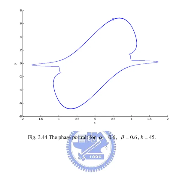
Fig. 3.39 The phase portrait of chaotic motion forα =β =0.6 with b=6.0. 29 Fig. 3.40~3.44 The phase portraits of periodic motions for α =β =0.6 with b=6.1,
6.5, 9.5, 20, 45 respectively. 30~32
Fig. 3.45 The bifurcation diagram for α =β =0.5. 33
Fig. 3.46 The phase portrait of chaotic motion forα =β =0.5 with b=2. 33 Fig. 3.47~3.49 The phase portraits of periodic motions for α =β =0.5 with b=6, 10,
15 respectively. 34~35
Fig. 3.50 The bifurcation diagram for α =β =0.4. 36
Fig. 3.51 The phase portrait of chaotic motion forα =β =0.4 with b=0.7. 36 Fig. 3.52、3.53 The phase portraits of periodic motions for α =β =0.4 with b=3.5,
6.0, respectively. 37
Fig. 3..54、3.55 The phase portraits of periodic motions for α =β =0.3 with b=0.01,
4.0, respectively. 38
Fig. 4.1 The phase portrait for replacing b by kcosx withα =β =1, a = 2, c = 10 43
Fig. 4.2 Error dynamics for Case 1. 43
Fig. 4.3 The phase portrait for replacing b by kcosx withα =β =0.9, a = 5, c = 5 44
Fig. 4.4 Error dynamics for Case 2. 44
Fig. 4.5 The phase portrait for replacing b by kcosx withα =β =0.8, a = 5, c = 5 45
Fig. 4.6 Error dynamics for Case 3. 45
Fig. 4.7 The phase portrait for replacing b by kcosx withα =β =0.7, a = 2.5, c = 35. 46
Fig. 4.8 Error dynamics for Case 4. 46
Fig. 4.9 The phase portrait for replacing b by kcosx withα =β =0.6, a = 2.5, c = 50 47
Fig. 4.10 Error dynamics for Case 5. 47
Fig. 4.11 The phase portrait for replacing b by kcosx withα =β =0.5, a = 2, c = 35. 48
Fig. 4.12 Error dynamics for Case 6. 48
Fig. 4.13 The phase portrait for replacing b by kcosx withα =β =0.4, a = 2, c = 65. 49
Fig. 4.14 Error dynamics for Case 7. 49
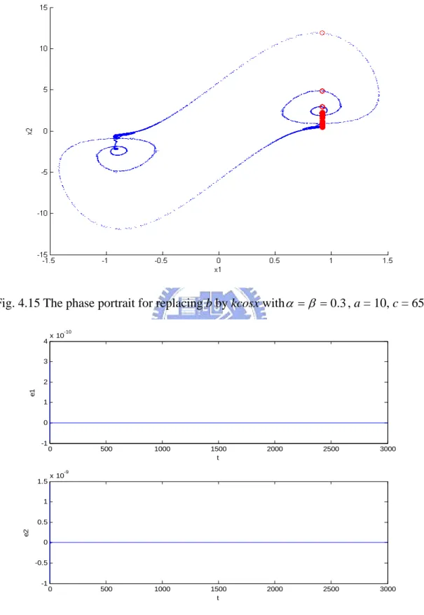
Fig. 4.15 The phase portrait for replacing b by kcosx withα =β =0.3, a = 10, c = 65. 50
Fig. 4.16 Error dynamics for Case 8. 50
Fig. 4.17 The phase portrait for replacing b by kcosx withα =β =0.2, a = 20, c = 55. 51
Fig. 4.24 Error dynamics for Case 2. 54 Fig. 4.25 The phase portrait for replacing b by kcosx withα =β =0.8, a = 5, c = 5 55
Fig. 4.26 Error dynamics for Case 3. 55
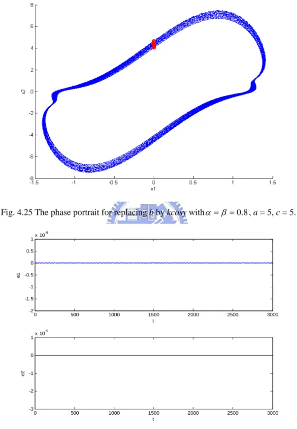
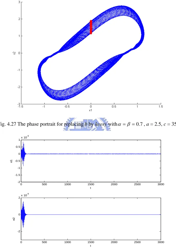
Fig. 4.27 The phase portrait for replacing b by kcosx withα =β =0.7, a = 2.5, c = 35. 56
Fig. 4.28 Error dynamics for Case 4. 56
Fig. 4.29 The phase portrait for replacing b by kcosx withα =β =0.6, a = 2.5, c = 50 57
Fig. 4.30 Error dynamics for Case 5. 57
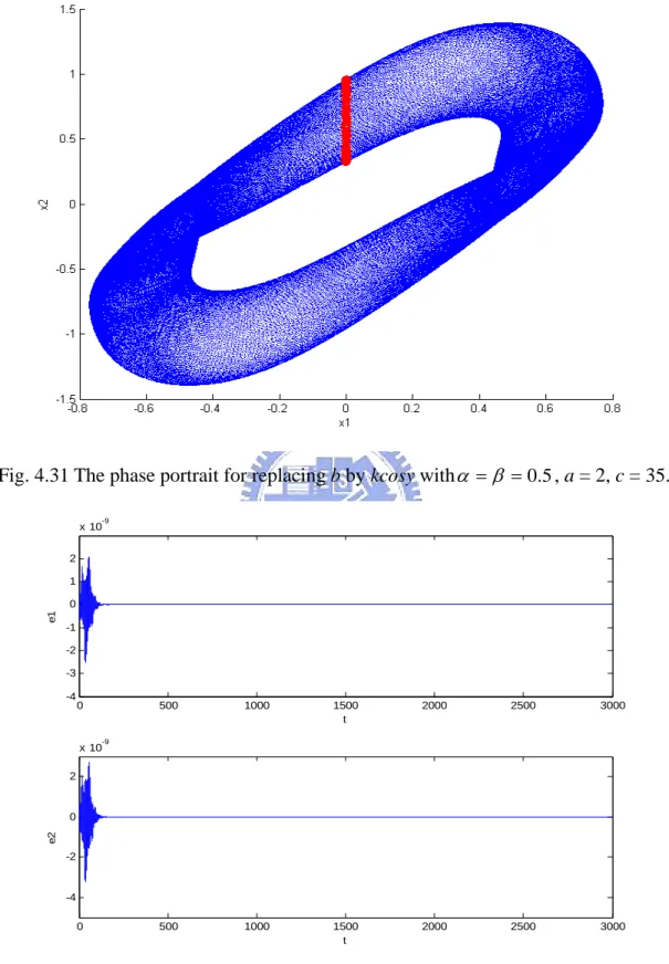
Fig. 4.31 The phase portrait for replacing b by kcosx withα =β =0.5, a = 2, c = 35 58
Fig. 4.32 Error dynamics for Case 6. 58
Fig. 4.33 The phase portrait for replacing b by kcosx withα =β =0.4,a = 2, c = 65. 59
Fig. 4.34 Error dynamics for Case 7. 59
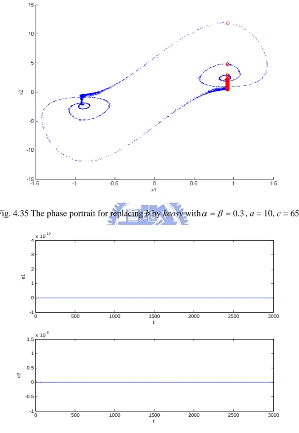
Fig. 4.35 The phase portrait for replacing b by kcosx withα =β =0.3, a = 10, c = 65. 60
Fig. 4.36 Error dynamics for Case 8. 60
Fig. 4.37 The phase portrait for replacing b by kcosx withα =β =0.2, a = 2, c = 1. 61
Fig. 4.38 Error dynamics for Case 9. 61
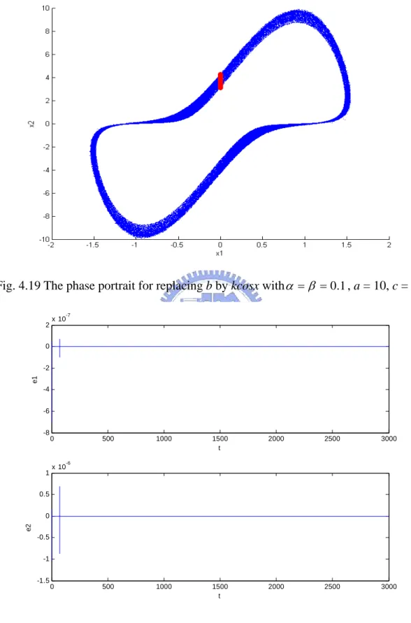
Fig. 4.39 The phase portrait for replacing b by kcosx withα =β =0.1, a = 10, c = 1 62
Fig. 4.40 Error dynamics for Case 10. 62
Fig. 4.41 The phase portrait for replacing b by kcosx withα =β =1, a = 2, c = 10 63
Fig. 4.42 Error dynamics for Case 1. 63
Fig. 4.43 The phase portrait for replacing b by kcosx withα =β =0.9, a = 5, c = 5 64
Fig. 4.44 Error dynamics for Case 2. 64
Fig. 4.45 The phase portrait for replacing b by kcosx withα =β =0.8, a = 10, c = 5 65
Fig. 4.46 Error dynamics for Case 3. 65
Fig. 4.48 Error dynamics for Case 4. 66 Fig. 4.49 The phase portrait for replacing b by kcosx withα =β =0.6, a = 2.5, c = 50 67
Fig. 4.50 Error dynamics for Case 5. 67
Fig. 4.51 The phase portrait for replacing b by kcosx withα =β =0.5, a = 5.5, c = 45. 68
Fig. 4.52 Error dynamics for Case 6. 68
Fig. 4.53 The phase portrait for replacing b by kcosx withα =β =0.4, a = 2, c = 65. 69
Fig. 4.54 Error dynamics for Case 7. 69
Fig. 4.55 The phase portrait for replacing b by kcosx withα =β =0.3, a = 4, c = 35. 70
Fig. 4.56 Error dynamics for Case 8. 70
Fig. 4.57 The phase portrait for replacing b by kcosx withα =β =0.2, a = 2, c = 1. 71
Fig. 4.58 Error dynamics for Case 9. 71
Fig. 4.59 The phase portrait for replacing b by kcosx withα =β =0.1, a = 2, c = 10. 72
Fig. 4.60 Error dynamics for Case 10. 72
Fig. 5.1(a) The bifurcation diagram forα =β =0.9. 76
Fig. 5.1(b)~(d) The phase portrait forα =β =0.9 with k = 0, 1.05, 1.1, respectively. 76
Fig. 5.2(a) The bifurcation diagram forα =β =0.8. 77
Fig. 5.2(b)~(d) The phase portrait forα =β =0.8 with k = 0, 0.87, 1.05, respectively. 77
Fig. 5.3(a) The bifurcation diagram forα =β =0.7. 78
Fig. 5.3(b)~(d) The phase portrait forα =β =0.7 with k = 0, 1.5, 1.6, respectively. 78
Fig. 5.4(a) The bifurcation diagram forα =β =0.6. 79
Fig. 5.4(b)~(d) The phase portrait forα =β =0.6 with k = 0, 1.291, 1.298,
respectively. 79
Fig. 5.5(a) The bifurcation diagram forα =β =0.5. 80
Fig. 5.5(b)~(d) The phase portrait forα =β =0.5 with k = 0, 1.35, 1.38, respectively. 80
Fig. 5.6(a) The bifurcation diagram forα =β =0.4. 81
Fig. 5.6(b)~(d) The phase portrait forα =β =0.4 with k = 0, 1.915, 1.93, respectively.
81
Fig. 5.7(a) The bifurcation diagram forα =β =0.3. 82
Fig. 5.10(b)~(d) The phase portrait forα =β =0.7 with k = 0, 1.205, 1.215,
respectively. 85
Fig. 5.11(a) The bifurcation diagram forα =β =0.6. 86
Fig. 5.11(b)~(d) The phase portrait forα =β =0.6 with k = 0, 0.95, 1.05, respectively.
86
Fig. 5.12(a) The bifurcation diagram forα =β =0.5. 87
Fig. 5.12(b)~(d) The phase portrait forα =β =0.5 with k = 0, 0.4, 0.6, respectively. 87
Fig. 5.13(a) The bifurcation diagram forα =β =0.4. 88
Fig. 5.13(b)~(d) The phase portrait forα =β =0.4 with k = 0, 1.25, 1.3, respectively. 88
Fig. 6.1(a) The bifurcation diagram forα =β =1. 93
Fig. 6.1(b) The phase portrait forα =β =1, b = 2.5. 93 Fig. 6.1(c) The phase portrait forα =β =1, k = 4. 93
Fig. 6.2(a) The bifurcation diagram forα =β =0.9. 94
Fig. 6.2(b) The phase portrait forα =β =0.9, b = 2.5. 94 Fig. 6.2(c) The phase portrait forα =β =0.9, k = 4. 94
Fig. 6.3(a) The bifurcation diagram forα =β =0.8. 95
Fig. 6.3(b) The phase portrait forα =β =0.8, b = 1.5. 95 Fig. 6.3(c) The phase portrait forα =β =0.8, k = 3. 95
Fig. 6.4(a) The bifurcation diagram forα =β =0.7. 96
Fig. 6.4(b) The phase portrait forα =β =0.7, b = 1.3. 96 Fig. 6.4(c) The phase portrait forα =β =0.7, k = 3.5. 96
Fig. 6.5(a) The bifurcation diagram forα =β =0.6. 97
Fig. 6.5(c) The phase portrait forα =β =0.6, k = 3.5. 97
Fig. 6.6(a) The bifurcation diagram forα =β =0.5. 98
Fig. 6.6(b) The phase portrait forα =β =0.5, b = 1. 98 Fig. 6.6(c) The phase portrait forα =β =0.5, k = 3. 98
Fig. 6.7(a) The bifurcation diagram forα =β =0.4. 99
Fig. 6.7(b) The phase portrait forα =β =0.4, b = 1.5. 99 Fig. 6.7(c) The phase portrait forα =β =0.4, k = 2.5. 99
Fig. 6.8(a) The bifurcation diagram forα =β =0.3. 100
Fig. 6.8(b) The phase portrait forα =β =0.3, b = 1.5. 100 Fig. 6.8(c) The phase portrait forα =β =0.3, k = 3.5. 100
Fig. 6.9(a) The bifurcation diagram forα =β =0.2. 101
Fig. 6.9(b) The phase portrait forα =β =0.2, b = 5. 101 Fig. 6.9(c) The phase portrait forα =β =0.2, k = 1. 101
Fig. 6.10(a) The bifurcation diagram forα =β =0.1. 102
Fig. 6.10(b) The phase portrait forα =β =0.1, b = 8. 102 Fig. 6.10(c) The phase portrait forα =β =0.1, k = 0.5. 102
useful in many applications such as fluid mixing [1], human brain [2], and heart beat regulation [3], etc. But like many other theories in science, the theory of chaos did not get enough attention for almost two decades, ever since Edward Lorenz reported his discovery of the theory in 1963. However, the invention of high-speed computers in the late 1970s and early 1980s brought about a major revolution in nonlinear dynamical theories in general, and chaos theory in particular that is why chaos theory developed in the natural sciences during the 1970s, and the social sciences during the 1980s.
Chaos synchronization [4-12] is a very important topic in the nonlinear [13-15] science and it has been developed extensively. Recently many scientists in various fields have been attracted to investigate chaos synchronization due to its application in a variety of fields such as secure communications, chemical, physical, and biological systems, neural networks, etc. So various synchronization schemes, such as variable structure control [16], parameters adaptive control [17-24], observer based control [25, 26], active control [27-33], nonlinear control [34, 35] and so on have been successfully applied to the chaos synchronization.
Fractional calculus is a 300-year-old mathematical topic. Although it has a long history, the applications of fractional calculus to physics and engineering are just a recent focus of interest [36]. In recent years, many scholars have devoted themselves to study the applications of the fractional order system to physics and engineering such as viscoelastic systems [37], dielectric polarization, and electromagnetic waves. More recently, there is a new trend to investigate the control [38] and dynamics [39-46] of the fractional order dynamical systems [47-49]. In [37] it has been shown that nonlinear chaotic systems still have chaotic behavior when their models become fractional. In [47], chaos control was investigated for fractional chaotic systems by the ‘‘back-stepping’’ method of nonlinear control design. In [48] and [49], it was found that chaos exists in a fractional order Chen system with order less than 3. Linear feedback control of chaos in
this system was also studied. In [41], chaos synchronization of fractional order chaotic systems was studied. The existence and uniqueness of solutions of initial value problems for fractional order differential equations have been studied in the literature [50-53].
In addition, anticontrol [54-60] of chaos have received great attention for many research activities in recent years and it is an interesting, new and challenging phenomenon [61-63]. As a reverse process of suppressing or eliminating chaotic behaviors in order to reduce the complexity of an individual system or a coupled system, anticontrol of chaos aims at creating or enhancing the system complexity for some special applications. More precisely, anticontrolling chaos is to generate some chaotic behaviors from a given system, which is non-chaotic or even is stable originally. By fully exploiting the intrinsic nonlinearity, this “control” technique provides another dimension for feedback systems design. Its potential applications can be easily found in many fields, including typically physics, biology, engineering, and medical as well as social sciences.
In this thesis, integral and fractional order modified heartbeat systems, i.e., van der Pol systems, are investigated. Chapter 2 presents a fractional derivative and the model of modified Van der Pol system. In Chapter 3, the dynamics of integral and fractional order modified van der Pol systems are investigated and the numerical results of periodic and chaotic phenomena are presented. The synchronizations of two uncoupled integral and fractional order chaotic modified van der Pol systems are achieved by parameter excited synchronization in Chapter 4. Anticontrol of chaos of fractional order modified van der Pol systems by addition of a constant term and addition of k|x|sinx term are discussed in Chapter 5. The parameter excited chaotization of integral and fractional order modified van der Pol systems is studied in Chapter 6. Finally, the conclusions are draw.
definition for a general fractional derivative is the Riemann-Liouville definition [64], which is given by 1 0 ( ) 1 ( ) ( ) ( ) q n t q n d f t d f d dt n q dt t τ q n τ τ − + = Γ −
∫
− (2.1) where is the gamma function and n is an integer such that . This definition is different from the usual intuitive definition of derivative. Fortunately, the basic engineering tool for analyzing linear systems, the Laplace transform, is still applicable and works as one would expect:) (⋅ Γ n−1<q<n
{
}
1 1 1 0 0 ( ) ( ) ( ) q n q q k q q k t d f t d f t L s L f t s dt dt − − − − − = k k = ⎧ ⎫ ⎡ ⎤ = − ⎨ ⎬ ⎢ ⎥ ⎩ ⎭∑
⎣ ⎦ , for all q, (2.2) where n is an integer such that n−1<q<n. Upon considering the initial conditions to be zero, this formula reduces to the more expected form{
}
( ) ( ) q q q d f t L s L dt ⎧ ⎫ = ⎨ ⎬ ⎩ ⎭ f t . (2.3) An efficient method is to approximate fractional operators by using standard integer order operators. In [65-69], an effective algorithm is developed to approximate fractional order transfer functions. Basically the idea is to approximate the system behavior based on frequency domain arguments. By utilizing frequency domain techniques based on Bode diagrams, one can obtain a linear approximation of the fractional order integrator, the order of which depends on the desired bandwidth and discrepancy between the actual and the approximate magnitude Bode diagrams. In Table 1 (See Appendix) of [70], approximations for qs
1
with q = 0.1 ~ 0.9 in steps 0.1 are given, with errors of approximately 2 dB. These approximations are used in the following simulations.
2.2 A modified heartbeat system and the corresponding fractional order system
Firstly, a heartbeat system, i.e. a van der Pol oscillator[71-73], driven by a periodic force is considered. The equation of motion can be written as:
0 sin ) 1 ( 2 − − = + + x a x x b t x& ϕ & ω & (2.4)
In Eq. (2.4), the linear term stands for a conservative harmonic force which determines the intrinsic oscillation frequency. The self-sustaining mechanism which is responsible for the perpetual oscillation rests on the nonlinear term. Energy exchange with the external agent depends on the magnitude of displacement |x| and on the sign of velocity
. During a complete cycle of oscillation, the energy is dissipated if displacement x(t) is large than one, and that energy is fed-in if |x| < 1. The time-dependent term stands for the external driving force with amplitude b and frequency
x&
ω.Eq. (2.4) can be rewritten as two first order equations:
⎩
⎨
⎧
+
−
+
−
=
=
t
b
y
x
a
x
y
y
x
ω
ϕ
(
1
2)
sin
&
&
(2.5) The modified heartbeat system, i.e. the modified van der Pol system, and its fractional order system studied in this paper are⎪ ⎪ ⎪ ⎩ ⎪ ⎪ ⎪ ⎨ ⎧ − − = = + − + − = = 3 2 ) 1 ( dz cz w w z bz y x a x dt y d y dt x d & & β β α α (2.6)
where α,β are integer numbers and fractional numbers respectively. System (2.6) can be separated into two parts:
⎪ ⎪ ⎩ ⎪⎪ ⎨ ⎧ + − + − = = bz y x a x dt y d y dt x d ) 1 ( 2 β β α α (2.7) and
time. Now d 0, z is a periodic motion of time but not a sinusoidal function of time. As a result, system (2.7) can be considered as a nonautonomous system with two states, while system (2.6) consisting of Eq. (2.7) and Eq. (2.8) can be considered as an autonomous system with four states. When
≠
1 = =β
α , Eq.(2.6) is the modified van der Pol system.
Chapter 3
Chaos in a Modified Heartbeat System and in Its Fractional
Order Systems
Chaos in a modified van der Pol system and in its fractional order systems is studied in this chapter. It is found that chaos exists both in the system and in the fractional order systems with total order from 1.8 down to 0.8 much less than the number of states of the system, two. By phase portraits, Poincaré maps and bifurcation diagrams, the chaotic behaviors of integral and fractional order modified van der Pol systems are presented.
In this chapter, phase portraits and bifurcation diagrams are studied for system (2.6) for α+β ≤2 and three parameters a, c, d are chosen as a = 5, c = 0.01, d = 0.001. A time step of 0.001 is used.
3.1 Chaos in a integral order modified heartbeat system
Let α =β =1. Fig. 3.1 shows the bifurcation diagram of the 2 order system. It is shown that chaos exists when b∈[0,1.0]. Fig. 3.2 is the phase portrait of chaotic motion with b = 1.0. Fig. 3.3 ~ 3.5 are phase portraits of periodic motions with , 1.5, 3, respectively. 1 . 1 = b
3.2 Chaos in a fractional order modified heartbeat system Case 1 Let α =0.9, β =0.9.
Fig. 3.6 shows the bifurcation diagram of the 1.8 order system. It is shown that chaos exists when b∈[0,9.7]. Fig. 3.7 is the phase portrait of chaotic motion with b = 9.7. Fig. 3.8 ~ 3.11 are phase portraits of periodic motions with b=9.8, 14, 23, 40 respectively.
Case 2 Let α=0.9, β =0.8.
Fig. 3.12 shows the bifurcation diagram of the 1.7 order system. It is shown that chaos exists when b∈[0,9.8]. Fig. 3.13 is the phase portrait of chaotic motion with b = 9.8. Fig. 3.14 ~ 3.17 are phase portraits of periodic motions
with b=10.2, 15, 23, 30, 45 respectively. Case 4 Let α =0.8, β =0.8.
Fig. 3.25 shows the bifurcation diagram of the 1.6 order system. It is shown that chaos exists when b∈[0,10.1]. Fig. 3.26 is the phase portrait of chaotic motion with b = 10.1. Fig. 3.27 ~ 3.31 are phase portraits of periodic motions with b=10.2, 14.5, 20, 35, 40 respectively.
Case 5 Let α =0.7, β =0.7.
Fig. 3.32 shows the bifurcation diagram of the 1.4 order system. It is shown that chaos exists when b∈[0,7.9]. Fig. 3.33 is the phase portrait of chaotic motion with b = 7.9. Fig. 3.34 ~ 3.37 are phase portraits of periodic motions with b=8.0, 15, 35, 40 respectively.
Case 6 Let α =0.6, β =0.6.
Fig. 3.38 shows the bifurcation diagram of the 1.2 order system. It is shown that chaos exists when b∈[0,6.0]. Fig. 3.39 is the phase portrait of chaotic motion with b = 6.0. Fig. 3.40 ~ 3.44 are phase portraits of periodic motions with b=6.1, 6.5, 9.5, 20, 45 respectively.
Case 7 Let α=0.5, β =0.5.
Fig. 3.45 shows the bifurcation diagram of the 1.0 order system. It is shown that chaos exists when b∈[0,4.2]. Fig. 3.46 is the phase portrait of chaotic motion with b = 2. Fig. 3.47 ~ 3.49 are phase portraits of periodic motions with b=6.0, 10, 15 respectively.
Case 8 Let α=0.4, β =0.4.
Fig. 3.50 shows the bifurcation diagram of the 0.8 order system. It is shown that chaos exists when b∈[0,1.8]. Fig. 3.51 is the phase portrait of chaotic motion with b = 0.7. Fig. 3.52 、 Fig. 3.53 are phase portraits of periodic
motions with , 1.3 respectively. When we tried to reduce the total order to 0.6, the phase portraits become periodic motions, as shown in Fig. 3.54 and Fig. 3.55, for any b value.
7 . 0 =
b
Chaos in modified van der Pol system and in its fractional order systems is studied in this chapter. It is found that the range of the chaos in the system gradually decreases as the total order number α+β decreases. Nine cases for 0.8≤
(
α+β)
≤2.0 are studied. The lowest total order for chaos existence in the system is found to be 0.8.-2.5 -2 -1.5 -1 -0.5 0 0.5 1 1.5 2 2.5 -10 -8 -6 -4 -2 0 2 4 x y
-2.5 -2 -1.5 -1 -0.5 0 0.5 1 1.5 2 2.5 -10 -8 -6 -4 -2 0 2 4 6 8 10 x y
Fig. 3.3 The phase portrait for α =β =1, b=1.1.
-2.5 -2 -1.5 -1 -0.5 0 0.5 1 1.5 2 2.5 -10 -8 -6 -4 -2 0 2 4 6 8 10 x y
-2.5 -2 -1.5 -1 -0.5 0 0.5 1 1.5 2 2.5 -10 -8 -6 -4 -2 0 x y
Fig. 3.6 The bifurcation diagram for α =0.9, β =0.9. -2 -1.5 -1 -0.5 0 0.5 1 1.5 2 -8 -6 -4 -2 0 2 4 6 8 x y
-2 -1.5 -1 -0.5 0 0.5 1 1.5 2 -8 -6 -4 -2 0 x y
Fig. 3.8 The phase portrait for α =0.9, β =0.9, b = 9.8.
-2 -1.5 -1 -0.5 0 0.5 1 1.5 2 -8 -6 -4 -2 0 2 4 6 8 x y
-2 -1.5 -1 -0.5 0 0.5 1 1.5 2 -10 -8 -6 -4 -2 0 2 4 6 8 10 y x
Fig. 3.10 The phase portrait for α =0.9, β =0.9, b = 23.
-2.5 -2 -1.5 -1 -0.5 0 0.5 1 1.5 2 2.5 -10 -8 -6 -4 -2 0 2 4 6 8 10 x y
-2 -1.5 -1 -0.5 0 0.5 1 1.5 2 -10 -8 -6 -4 -2 0 2 4 6 x y
-2 -1.5 -1 -0.5 0 0.5 1 1.5 2 -10 -8 -6 -4 -2 0 2 4 6 8 10 x y
Fig. 3.14 The phase portrait for α =0.9, β =0.8, b = 9.9.
-2 -1.5 -1 -0.5 0 0.5 1 1.5 2 -10 -8 -6 -4 -2 0 2 4 6 8 10 x y
-2 -1.5 -1 -0.5 0 0.5 1 1.5 2 -15 -10 -5 0 x y
Fig. 3.16 The phase portrait for α =0.9, β =0.8, b = 25.
-2 -1.5 -1 -0.5 0 0.5 1 1.5 2 -10 -8 -6 -4 -2 0 2 4 6 8 10 x y
Fig. 3.18 The bifurcation diagram for α =0.8, β =0.9. -2 -1.5 -1 -0.5 0 0.5 1 1.5 2 -8 -6 -4 -2 0 2 4 6 8 x y
-2 -1.5 -1 -0.5 0 0.5 1 1.5 2 -8 -6 -4 -2 0 x y
Fig. 3.20 The phase portrait for α =0.8, β =0.9, b = 10.2.
-2 -1.5 -1 -0.5 0 0.5 1 1.5 2 -8 -6 -4 -2 0 2 4 6 8 x y
-2 -1.5 -1 -0.5 0 0.5 1 1.5 2 -8 -6 -4 -2 0 2 4 6 8 x y
Fig. 3.22 The phase portrait for α =0.8, β =0.9, b = 23.
-2 -1.5 -1 -0.5 0 0.5 1 1.5 2 -8 -6 -4 -2 0 2 4 6 8 x y
-2.5 -2 -1.5 -1 -0.5 0 0.5 1 1.5 2 2.5 -8 -6 -4 -2 0 x y
Fig. 3.25 The bifurcation diagram for α =0.8, β =0.8.
-1.5 -1 -0.5 0 0.5 1 1.5 -8 -6 -4 -2 0 2 4 6 8 x y
-1.5 -1 -0.5 0 0.5 1 1.5 -8 -6 -4 -2 0 x y
Fig. 3.27 The phase portrait for α =0.8, β =0.8, b = 10.2.
-1.5 -1 -0.5 0 0.5 1 1.5 -8 -6 -4 -2 0 2 4 6 8 x y
-1.5 -1 -0.5 0 0.5 1 1.5 -8 -6 -4 -2 0 2 4 6 8 x y
Fig. 3.29 The phase portrait for α =0.8, β =0.8, b = 20.
-2 -1.5 -1 -0.5 0 0.5 1 1.5 2 -8 -6 -4 -2 0 2 4 6 8 x y
-2.5 -2 -1.5 -1 -0.5 0 0.5 1 1.5 2 2.5 -8 -6 -4 -2 0 x y
0 5 10 15 20 25 30 35 40 45 50 4.2 4.4 4.6 4.8 5 5.2 5.4 5.6 5.8
Fig. 3.32 The bifurcation diagram for α=0.7, β =0.7.
-1.5 -1 -0.5 0 0.5 1 1.5 -6 -4 -2 0 2 4 6 x y
-1.5 -1 -0.5 0 0.5 1 1.5 -6 -4 -2 0 x y
Fig. 3.34 The phase portrait for α =0.7, β =0.7, b = 8.0.
-1.5 -1 -0.5 0 0.5 1 1.5 -6 -4 -2 0 2 4 6 x y
-2 -1.5 -1 -0.5 0 0.5 1 1.5 2 -6 -4 -2 0 2 4 6 x y
Fig. 3.36 The phase portrait for α =0.7, β =0.7, b = 35.
-2 -1.5 -1 -0.5 0 0.5 1 1.5 2 -6 -4 -2 0 2 4 6 x y
Fig. 3.38 The bifurcation diagram for α=0.6, β =0.6. -1.5 -1 -0.5 0 0.5 1 1.5 -6 -4 -2 0 2 4 6 x y
-1.5 -1 -0.5 0 0.5 1 1.5 -6 -4 -2 0 2 4 6 x y
Fig. 3.40 The phase portrait for α =0.6, β =0.6, b = 6.1.
-1.5 -1 -0.5 0 0.5 1 1.5 -6 -4 -2 0 2 4 6 x y
-1.5 -1 -0.5 0 0.5 1 1.5 -6 -4 -2 0 x y
Fig. 3.42 The phase portrait for α =0.6, β =0.6, b = 9.5.
-1.5 -1 -0.5 0 0.5 1 1.5 -6 -4 -2 0 2 4 6 x y
-2 -1.5 -1 -0.5 0 0.5 1 1.5 2 -8 -6 -4 -2 0 2 4 6 8 x y
-1.5 -1 -0.5 0 0.5 1 1.5 -5 -4 -3 -2 -1 0 1 2 3 x y
-1.5 -1 -0.5 0 0.5 1 1.5 -6 -4 -2 0 2 4 6 x y
Fig. 3.47 The phase portrait for α =0.5, β =0.5, b = 6.
-1.5 -1 -0.5 0 0.5 1 1.5 -6 -4 -2 0 2 4 6 x y
-1.5 -1 -0.5 0 0.5 1 1.5 -6 -4 -2 0 x y
0 1 2 3 4 5 6 7 8 9 10 4 4.5 5 b y
Fig. 3.50 The bifurcation diagram for α =0.4, β =0.4.
-1.5 -1 -0.5 0 0.5 1 1.5 -5 -4 -3 -2 -1 0 1 2 3 4 5 x y
Fig. 3.54 The phase portrait for α=0.3, β =0.3, b = 0.7.
-1.5 -1 -0.5 0 0.5 1 1.5 -5 -4 -3 -2 -1 0 1 2 3 4 5 x y
In this chapter, the synchronizations of two uncoupled integral and fractional order chaotic modified heartbeat systems, i.e. modified van der Pol systems, are achieved by replacing the corresponding parameters of two systems by the same function of the chaotic state variables of a third chaotic system. It is named parameter excited synchronization which can be successfully obtained for very low total fractional order 0.2. Numerical simulations are illustrated by phase portraits, Poincaré maps and state error plots.
4.1 The scheme of parameter excited chaos synchronizations
In this section, both parameters b of two identical modified fractional order van der Pol systems with different initial conditions
⎪ ⎪ ⎪ ⎩ ⎪ ⎪ ⎪ ⎨ ⎧ − − = = + − + − = = 3 1 1 1 1 1 1 1 2 1 1 1 1 1 ) 1 ( dz cz w w z bz y x a x dt y d y dt x d & & β β α α (4.1) ⎪ ⎪ ⎪ ⎩ ⎪ ⎪ ⎪ ⎨ ⎧ − − = = + − + − = = 3 2 2 2 2 2 2 2 2 2 2 2 2 2 ) 1 ( dz cz w w z bz y x a x dt y d y dt x d & & β β α α (4.2)
are replaced by the same cosine function of state variables of a third system (2.6). We study the parameter excited chaos synchronization for variousα,β . The parameters a, c of systems (4.1) and (4.2) are adjusted to achieve synchronization for differentαandβ .
when , synchronization is obtained. A time step of 0.001 is used. Three cases are studied.
∞ →
t
4.2 Parameter Excited Chaos Synchronizations by kcosx、kcosy、kcosxcosy
Then, the corresponding parameters b of two uncoupled identical integral and fractional order chaotic modified van der Pol systems will be replaced by kcosx, kcosy,
kcosxcosy, where x, y are the states of a third identical system (2.6).
4.2.1 Parameter Excited Chaos Synchronizations by kcosx
Let the parameter b of Eqs. (4.1) and (4.2) be replaced by kcosx where x is the state variable of system (2.6). Parameter k is chosen as k = 0.5.
Case 1 Let α =β =1. Fig. 4.1 shows that the chaos exists when a = 2, c = 10. Fig. 4.2 shows the error dynamics for synchronization.
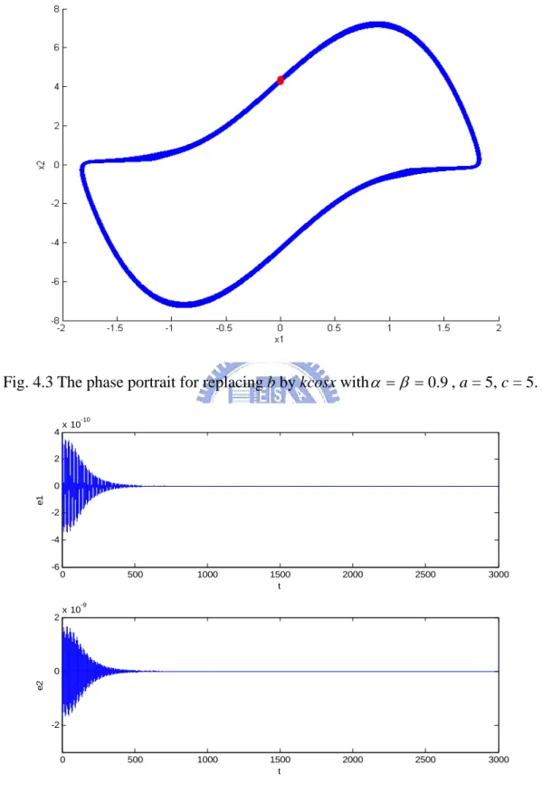
Case 2 Let α =β =0.9. Fig. 4.3 shows that the chaos exists when a = 5, c = 5. Fig. 4.4 shows the error dynamics for synchronization.
Case 3 Let α =β =0.8. Fig. 4.5 shows that the chaos exists when a = 5, c = 5. Fig. 4.6 shows the error dynamics for synchronization.
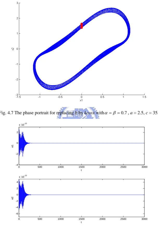
Case 4 Let α =β =0.7. Fig. 4.7 shows that the chaos exists when a = 2.5, c = 35. Fig. 4.8 shows the error dynamics for synchronization.
Case 5 Let α =β =0.6. Fig. 4.9 shows that the chaos exists when a = 2.5, c = 50. Fig. 4.10 shows the error dynamics for synchronization.
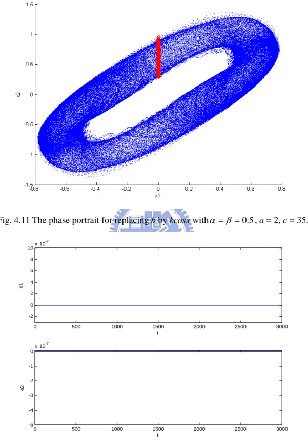
Case 6 Let α =β =0.5. Fig. 4.11 shows that the chaos exists when a = 2, c = 35. Fig. 4.12 shows the error dynamics for synchronization.
Case 7 Let α =β =0.4. Fig. 4.13 shows that the chaos exists when a = 2, c = 65. Fig. 4.14 shows the error dynamics for synchronization.
Case 8 Let α =β =0.3. Fig. 4.15 shows that the chaos exists when a = 10, c = 65. Fig. 4.16 shows the error dynamics for synchronization.
Case 9 Let α =β =0.2. Fig. 4.17 shows that the chaos exists when a = 20, c = 55. Fig. 4.18 shows the error dynamics for synchronization.
Case 10 Let α =β =0.1. Fig. 4.19 shows that the chaos exists when a = 10, c = 0.5. Fig. 4.20 shows the error dynamics for synchronization.
Case 2 Let α =β =0.9. Fig. 4.23 shows that the chaos exists when a = 5, c = 5. Fig. 4.24 shows the error dynamics for synchronization.
Case 3 Let α =β =0.8. Fig. 4.25 shows that the chaos exists when a = 5, c = 5. Fig. 4.26 shows the error dynamics for synchronization.
Case 4 Let α =β =0.7. Fig. 4.27 shows that the chaos exists when a = 2.5, c = 35. Fig. 4.28 shows the error dynamics for synchronization.
Case 5 Let α =β =0.6. Fig. 4.29 shows that the chaos exists when a = 2.5, c = 50. Fig. 4.30 shows the error dynamics for synchronization.
Case 6 Let α =β =0.5. Fig. 4.31 shows that the chaos exists when a = 2, c = 35. Fig. 4.32 shows the error dynamics for synchronization.
Case 7 Let α =β =0.4. Fig. 4.33 shows that the chaos exists when a = 2, c = 65. Fig. 4.34 shows the error dynamics for synchronization.
Case 8 Let α =β =0.3. Fig. 4.35 shows that the chaos exists when a = 5, c = 5. Fig. 4.36 shows the error dynamics for synchronization.
Case 9 Let α =β =0.2. Fig. 4.37 shows that the chaos exists when a = 20, c = 55. Fig. 4.38 shows the error dynamics for synchronization.
Case 10 Let α =β =0.1. Fig. 4.39 shows that the chaos exists when a = 10, c = 1. Fig. 4.40 shows the error dynamics for synchronization.
4.2.3 Parameter Excited Chaos Synchronizations by kcosxcosy
Let the parameter b of Eqs. (4.1) and (4.2) be replaced by kcosxcosy where x, y are the state variables of system (6). Parameter k is chosen as k = 0.5.
Case 1 Let α =β =1. Fig. 4.41 shows that the chaos exists when a = 2, c = 10. Fig. 4.42 shows the error dynamics for synchronization.
Case 2 Let α =β =0.9. Fig. 4.43 shows that the chaos exists when a = 5, c = 5. Fig. 4.44 shows the error dynamics for synchronization.
Case 3 Let α =β =0.8. Fig. 4.45 shows that the chaos exists when a = 10, c = 5. Fig. 4.46 shows the error dynamics for synchronization.
Case 4 Let α =β =0.7. Fig. 4.47 shows that the chaos exists when a = 2.5, c = 35. Fig. 4.48 shows the error dynamics for synchronization.
Case 5 Let α =β =0.6. Fig. 4.49 shows that the chaos exists when a = 2.5, c = 50. Fig. 4.50 shows the error dynamics for synchronization.
Case 6 Let α =β =0.5. Fig. 4.51 shows that the chaos exists when a = 5.5, c = 45. Fig. 4.52 shows the error dynamics for synchronization.
Case 7 Let α =β =0.4. Fig. 4.53 shows that the chaos exists when a = 2, c = 65. Fig. 4.54 shows the error dynamics for synchronization.
Case 8 Let α =β =0.3. Fig. 4.55 shows that the chaos exists when a = 4, c = 35. Fig. 4.56 shows the error dynamics for synchronization.
Case 9 Let α =β =0.2. Fig. 4.57 shows that the chaos exists when a = 2, c = 1. Fig. 4.58 shows the error dynamics for synchronization.
Case 10 Let α =β =0.1. Fig. 4.59 shows that the chaos exists when a = 2, c = 10. Fig. 4.60 shows the error dynamics for synchronization.
In this paper, parameter excited chaos synchronizations of uncoupled integral and fractional order modified van der Pol systems are studied by means of phase portraits, Poincaré maps and error dynamics plots. It is found that this approach is very effective even for very low total fractional order 0.2.
0 500 1000 1500 2000 2500 3000 -8 -6 -4 t e1 0 500 1000 1500 2000 2500 3000 -4 -2 0 2 4 6 t e2
Fig. 4.3 The phase portrait for replacing b by kcosx withα =β =0.9, a = 5, c = 5. 0 500 1000 1500 2000 2500 3000 -6 -4 -2 0 2 4x 10 -10 t e1 0 500 1000 1500 2000 2500 3000 -2 0 2x 10 -9 t e2
0 500 1000 1500 2000 2500 3000 -2 -1.5 -1 -0.5 t e1 0 500 1000 1500 2000 2500 3000 -3 -2 -1 0 1x 10 -6 t e2
Fig. 4.7 The phase portrait for replacing b by kcosx withα =β =0.7, a = 2.5, c = 35. 0 500 1000 1500 2000 2500 3000 -4 -2 0 2 x 10⁻¹⁰ t e1 0 500 1000 1500 2000 2500 3000 -6 -4 -2 0 2 4 x 10⁻¹⁰ t e2
0 500 1000 1500 2000 2500 3000 -3 -2 -1 t e1 0 500 1000 1500 2000 2500 3000 -6 -4 -2 0 2 4x 10 -10 t e2
Fig. 4.11 The phase portrait for replacing b by kcosx withα =β =0.5, a = 2, c = 35. 0 500 1000 1500 2000 2500 3000 -2 0 2 4 6 8 10x 10 -7 t e1 0 500 1000 1500 2000 2500 3000 -5 -4 -3 -2 -1 0 x 10-7 t e2
0 500 1000 1500 2000 2500 3000 -4 -2 t e1 0 500 1000 1500 2000 2500 3000 -4 -2 0 2 x 10⁻¹⁰ t e2
Fig. 4.15 The phase portrait for replacing b by kcosx withα =β =0.3, a = 10, c = 65. 0 500 1000 1500 2000 2500 3000 -1 0 1 2 3 4x 10 -10 t e1 0 500 1000 1500 2000 2500 3000 -1 -0.5 0 0.5 1 1.5x 10 -9 t e2
0 500 1000 1500 2000 2500 3000 3500 4000 4500 5000 -5 -4 -3 t e1 0 500 1000 1500 2000 2500 3000 3500 4000 4500 5000 0 10 20 30 t e2
Fig. 4.19 The phase portrait for replacing b by kcosx withα =β =0.1, a = 10, c = 0.5. 0 500 1000 1500 2000 2500 3000 -8 -6 -4 -2 0 2x 10 -7 t e1 0 500 1000 1500 2000 2500 3000 -1.5 -1 -0.5 0 0.5 1x 10 -6 t e2
-2.5 -2 -1.5 -1 -0.5 0 0.5 1 1.5 2 2.5 -5 -4 -3 -2 -1 0 x1 x2
Fig. 4.21 The phase portrait for replacing b by kcosy withα =β =1, a = 2, c = 10.
0 500 1000 1500 2000 2500 3000 -8 -6 -4 -2 0 2 4 t e1 0 500 1000 1500 2000 2500 3000 -5 0 5 t e2
-2 -1.5 -1 -0.5 0 0.5 1 1.5 2 -8 -6 -4 -2 0 2 4 6 8 x1 x2
Fig. 4.23 The phase portrait for replacing b by kcosy withα =β =0.9, a = 5, c = 5.
0 500 1000 1500 2000 2500 3000 -5 -4 -3 -2 -1 0 1 x 10⁻⁸ t e1 0 500 1000 1500 2000 2500 3000 -10 -5 0 5 x 10⁻⁸ t e2
0 500 1000 1500 2000 2500 3000 -2 -1.5 -1 -0.5 t e1 0 500 1000 1500 2000 2500 3000 -3 -2 -1 0 1x 10 -5 t e2
Fig. 4.27 The phase portrait for replacing b by kcosy withα =β =0.7, a = 2.5, c = 35. 0 500 1000 1500 2000 2500 3000 -2 -1.5 -1 -0.5 0 0.5 1x 10 -9 t e1 0 500 1000 1500 2000 2500 3000 -2 0 2x 10 -9 t e2
0 500 1000 1500 2000 2500 3000 -3 -2 -1 t e1 0 500 1000 1500 2000 2500 3000 -6 -4 -2 0 2 4x 10 -9 t e2
Fig. 4.31 The phase portrait for replacing b by kcosy withα =β =0.5, a = 2, c = 35. 0 500 1000 1500 2000 2500 3000 -4 -3 -2 -1 0 1 2 x 10⁻⁹ t e1 0 500 1000 1500 2000 2500 3000 -4 -2 0 2 x 10⁻⁹ t e2
0 500 1000 1500 2000 2500 3000 -4 -2 t e1 0 500 1000 1500 2000 2500 3000 -4 -2 0 2 4x 10 -8 t e2
Fig. 4.35 The phase portrait for replacing b by kcosy withα =β =0.3, a = 10, c = 65. 0 500 1000 1500 2000 2500 3000 -1 0 1 2 3 4x 10 -10 t e1 0 500 1000 1500 2000 2500 3000 -1 -0.5 0 0.5 1 1.5x 10 -9 t e2
0 500 1000 1500 2000 2500 3000 -5 t e1 0 500 1000 1500 2000 2500 3000 -5 0 5 10 15x 10 -9 t e2
Fig. 4.39 The phase portrait for replacing b by kcosy withα =β =0.1, a = 10, c = 1. 0 500 1000 1500 2000 2500 3000 -6 -4 -2 0 2 4 t e1 0 500 1000 1500 2000 2500 3000 -30 -20 -10 0 10 20 t e2
0 500 1000 1500 2000 2500 3000 -10 -8 -6 -4 t e1 0 500 1000 1500 2000 2500 3000 -6 -4 -2 0 2 4 t e2
Fig. 4.43 The phase portrait for replacing b by kcosxcosy withα =β =0.9, a = 5, c = 5. 0 500 1000 1500 2000 2500 3000 -1 0 1x 10 -9 t e1 0 500 1000 1500 2000 2500 3000 -5 0 x 10-9 t e2
0 500 1000 1500 2000 2500 3000 -4 -2 t e1 0 500 1000 1500 2000 2500 3000 -4 -3 -2 -1 0 1 2 x 10⁻⁹ t e2
Fig. 4.47 The phase portrait for replacing b by kcosxcosy withα =β =0.7, a = 2.5, c = 35. 0 500 1000 1500 2000 2500 3000 -4 -3 -2 -1 0 1 x 10⁻¹⁰ t e1 0 500 1000 1500 2000 2500 3000 -6 -4 -2 0 2 4x 10 -10 t e2
0 500 1000 1500 2000 2500 3000 -3 -2 -1 0 t e1 0 500 1000 1500 2000 2500 3000 -4 -2 0 2 x 10⁻¹⁰ t e2
Fig. 4.51 The phase portrait for replacing b by kcosxcosy withα =β =0.5, a = 5.5, c = 45. 0 500 1000 1500 2000 2500 3000 -8 -6 -4 -2 0 x 10-10 t e1 0 500 1000 1500 2000 2500 3000 -5 -4 -3 -2 -1 0 x 10-9 t e2
0 500 1000 1500 2000 2500 3000 -6 -4 -2 t e1 0 500 1000 1500 2000 2500 3000 -1 0 1 2 3 x 10-11 t e2
Fig. 4.55 The phase portrait for replacing b by kcosxcosy withα =β =0.3, a = 4, c = 35. 0 500 1000 1500 2000 2500 3000 -10 -8 -6 -4 -2 0 x 10-9 t e1 0 500 1000 1500 2000 2500 3000 -20 -15 -10 -5 0 x 10-9 t e2
0 500 1000 1500 2000 2500 3000 -0.5 0 0.5 t e1 0 500 1000 1500 2000 2500 3000 -6 -4 -2 0 2 4 t e2
Fig. 4.59 The phase portrait for replacing b by kcosxcosy withα =β =0.1, a = 2, c = 10. 0 500 1000 1500 2000 2500 3000 -2 0 2 4 6 8 x 10⁻¹⁰ t e1 0 500 1000 1500 2000 2500 3000 -15 -10 -5 0 5x 10 -10 t e2
Anticontrol of chaos of fractional order modified heartbeat systems is studied. Anticontrol of chaos is making a non-chaotic dynamical system chaotic, i.e., the regular behavior will be destroyed and replaced by chaotic behavior. Addition of a constant term and addition of k|x|sinx term where x is a state of the system are used to anticontrol the system effectively. By applying numerical results, phase portrait, Poincaré maps and bifurcation diagrams a variety of the phenomena of the chaotic motion can be presented.
5.1 Anticontrol of chaos by addition of a constant term
We add a constant term k in the second equation of system (2.6) and it become:
⎪ ⎪ ⎪ ⎩ ⎪ ⎪ ⎪ ⎨ ⎧ − − = = + + − + − = = 3 2 ) 1 ( dz cz w w z k bz y x a x dt y d y dt x d & & β β α α (5.1)
In system (5.1), the parameter b is adjusted to achieve periodic motion for different
αandβ when k = 0. a, c, d are fixed and they are chosen as a= 5, c = 0.01, d = 0.001.
Case 1 Letα =β =0.9, b = 2.5, andk∈[0.9,1.2]. Fig 5.1(a) shows the bifurcation diagram of the 1.8 order system. Fig 5.1(b) ~ 5.1(d) are the phase portraits
with k = 0, 1.05, 1.1.
Case 2 Letα =β =0.8, b = 1.5, andk∈[0.6,1.2]. Fig 5.2(a) shows the bifurcation diagram of the 1.6 order system. Fig 5.2(b) ~ 5.2(d) are the phase portraits with k = 0, 0.87, 1.05.
Case 3 Letα =β =0.7, b = 1.3, andk∈[0.1,1.6]. Fig 5.3(a) shows the bifurcation diagram of the 1.4 order system. Fig 5.3(b) ~ 5.3(d) are the phase portraits with k = 0, 1.5, 1.6.
Case 4 Letα =β =0.6, b = 1, andk∈[1.282,1.312]. Fig 5.4(a) shows the bifurcation diagram of the 1.2 order system. Fig 5.4(b) ~ 5.4(d) are the phase portraits with k = 0, 1.291, 1.298.
Case 5 Letα =β =0.5, b = 1, andk∈[1.32,1.42]. Fig 5.5(a) shows the bifurcation diagram of the 1.0 order system. Fig 5.5(b) ~ 5.5(d) are the phase portraits with k = 0, 1.35, 1.38.
Case 6 Letα =β =0.4, b = 1.5, andk∈[1.88,1.94]. Fig 5.6(a) shows the bifurcation diagram of the 0.8 order system. Fig 5.6(b) ~ 5.6(d) are the phase portraits with k = 0, 1.915, 1.93.
Case 7 Letα =β =0.3, b = 1.5, andk∈[1.89,1.98]. Fig 5.7(a) shows the bifurcation diagram of the 0.6 order system. Fig 5.7(b) ~ 5.7(d) are the phase portraits with k = 0, 1.9, 1.94.
5.2 Anticontrol of chaos by addition of a nonlinear term
We add a non-linear term k|x|sinx in the second equation of system (2.6) and it become: ⎪ ⎪ ⎪ ⎩ ⎪ ⎪ ⎪ ⎨ ⎧ − − = = + + − + − = = 3 2 sinx | x | k ) 1 ( dz cz w w z bz y x a x dt y d y dt x d & & β β α α (5.2)
In system (5.2), the parameter b is also adjusted to achieve periodic motion for differentαandβ when k = 0. , c, d are fixed as 5.1. a
Case 1 Letα =β =0.9, b = 2.5, andk∈[0.2,0.4]. Fig 5.8(a) shows the bifurcation diagram of the 1.8 order system. Fig 5.8(b) ~ 5.8(d) are the phase portraits with k = 0, 0.35, 0.4.
Case 2 Letα =β =0.8, b = 2.5, andk∈[1.0,1.3]. Fig 5.9(a) shows the bifurcation diagram of the 1.6 order system. Fig 5.9(b) ~ 5.9(d) are the phase portraits with k = 0, 1.03, 1.2.
Case 3 Letα =β =0.7, b = 0.5, andk∈[1.19,1.24]. Fig 5.10(a) shows the bifurcation diagram of the 1.4 order system. Fig 5.10(b) ~ 5.10(d) are the phase portraits
diagram of the 1.0 order system. Fig 5.12(b) ~ 5.12(d) are the phase portraits with k = 0, 0.4, 0.6.
Case 6 Letα =β =0.4, b = 1, andk∈[1.16,1.37]. Fig 5.13(a) shows the bifurcation diagram of the 0.8 order system. Fig 5.13(b) ~ 5.13(d) are the phase portraits with k = 0, 1.25, 1.3.
Anticontrol of chaos in the fractional order systems of a modified van der Pol system are studied in the chapter. An efficient way to transform a non-chaotic dynamical system into a chaotic one is easily made by addition of a constant term or by addition of
k|x|sinx term where x is a state variable of the system. It is found that chaos exists in the
fractional order systems with order from 1.8 down to 0.6 for the addition of constant term, and from 1.8 down to 0.8 for the addition of k|x|sinx term.
0.9 0.95 1 1.05 1.1 1.15 1.2 1.25 0 0.5 1 1.5 2 2.5 y y k k (a) y x (b) k = 0 (c) k = 1.05 (d) k = 1.1
Fig 5.1 The bifurcation diagram forα =β =0.9 and phase portrait forα =β =0.9 with
k = 0, k = 1.05, k = 1.1 respectively.
y y
y x (b) k = 0 y y x x (c) k = 0.87 (d) k = 1.05
Fig 5.2 The bifurcation diagram forα =β =0.8 and phase portrait forα =β =0.8 with
x k (a) y x (b) k = 0 y y (c) k = 1.5 (d) k = 1.6
Fig 5.3 The bifurcation diagram forα =β =0.7 and phase portrait forα =β =0.7 with
k = 0, 1.5, 1.6, respectively.
y
x
(b) k = 0
(c) k = 1.291 (d) k =1.298
Fig 5.4 The bifurcation diagram forα =β =0.6 and phase portrait forα =β =0.6 with
k = 0, 1.291, 1.298, respectively.
y y
1.32 1.34 1.36 1.38 1.4 1.42 1.44 -6 -5.8 -5.6 -5.4 -5.2 -5 -4.8 -4.6 -4.4 -4.2 y k y k (a) y x (b) k = 0 y y (c) k = 1.35 (d) k = 1.38
Fig 5.5 The bifurcation diagram forα =β =0.5 and phase portrait forα =β =0.5 with
k = 0, 1.35, 1.38, respectively.
y
x
(b) k = 0
y y
(c) k = 1.915 (d) k = 1.93
Fig 5.6 The bifurcation diagram forα =β =0.4 and phase portrait forα =β =0.4 with
k = 0, 1.915, 1.93, respectively.
1.88 1.9 1.92 1.94 1.96 1.98 2 -0.82 -0.81 -0.8 -0.79 -0.78 -0.77 -0.76 -0.75 x k x k (a) y x (b) k = 0 (c) k = 1.9 (d) k =1.94
Fig 5.7 The bifurcation diagram forα =β =0.3 and phase portrait forα =β =0.3 with
k = 0, 1.9, 1.94, respectively.
y y
0.2 0.22 0.24 0.26 0.28 0.3 0.32 0.34 0.36 0.38 0.4 -9 -8.5 k k (a) y (b) k = 0 x (c) k = 0.35 (d) k =0.4
Fig 5.8 The bifurcation diagram forα =β =0.9and phase portrait forα =β =0.9with
k = 0, 0.35, 0.4, respectively.
y y
1 1.05 1.1 1.15 1.2 1.25 1.3 1.35 1.4 -8.5 -8 -7.5 -7 -6.5 -6 -5.5 -5 -4.5 -4 y k y k (a) y x (b) k = 0 y y (c) k = 1.03 (d) k = 1.2
Fig 5.9 The bifurcation diagram forα =β =0.8and phase portrait forα =β =0.8 with
k = 0, 1.03, 1.2, respectively.
1.19 1.195 1.2 1.205 1.21 1.215 1.22 1.225 1.23 1.235 1.24 -0.9 -0.8 k k (a) y x (b) k = 0 (c) k = 1.205 (d) k = 1.215
Fig 5.10 The bifurcation diagram forα =β =0.7 and The phase portrait forα =β =0.7
with k = 0, 1.205, 1.215, respectively.
y y
0.8 0.85 0.9 0.95 1 1.05 1.1 1.15 1.2 1.25 1.3 -1.4 -1.2 -1 -0.8 -0.6 -0.4 -0.2 0 y k y k (a) y x (b) k = 0 y y (c) k = 0.95 (d) k = 1.05
Fig 5.11 The bifurcation diagram forα =β =0.6and phase portrait forα =β =0.6 with
k = 0, 0.95, 1.05, respectively.
y
x
(b) k = 0
(c) k = 0.4 (d) k = 0.6
Fig 5.12 The bifurcation diagram forα =β =0.5 and phase portrait forα =β =0.5
with k = 0, 0.4, 0.6, respectively.
y y
y k (a) y x (b) k = 0 (c) k = 1.25 (d) k = 1.3
Fig 5.13 The bifurcation diagram forα =β =0.4and phase portrait forα =β =0.4 with
k = 0, 1.25, 1.3, respectively.
y y
Chaotization of integral and fractional order modified heartbeat systems by replacing the parameter of modified heartbeat system by the function of the chaotic state variables of a second chaotic nano resonator system is studied. It is named parameter excited chaotization which can be successfully obtained for very low total fractional order 0.2. By phase portraits, Poincaré maps and bifurcation diagrams, the simulation results of fractional order modified van der Pol systems are presented.
6.1 A nano resonator system and the chaotization scheme
Chaotization, i.e. anticontrol of chaos, is making a non-chaotic dynamical system chaotic. This means that the regular behavior will be destroyed and replaced by chaotic behavior.
Nano resonator system is a modified form of nonlinear damped Mathieu system which is obtained when the nano Mathieu oscillator has nonlinear time-dependent spring constant. The nonlinear damped Mathieu system is a nonautonomous system with two states x and y:
⎪ ⎪ ⎩ ⎪⎪ ⎨ ⎧ + − + − + − = = t h gy x t f e x t f e dt dy y dt dx 2 3 1 1 ) ( sin ) sin sin ( ω ω ω (6.1)
where a, b, c, d are constant parameters, and ω1, ω2 are circular frequencies. Let
1
ω =ω2=ω, and replace sin tω by z which is the periodic time function solution of the nonlinear oscillator
⎪ ⎪ ⎩ ⎪⎪ ⎨ ⎧ − − = = 3 jz iz dt dw w dt dz (6.2)
where i, j are constants. Then we have the modified nonlinear damped Mathieu system, i.e. the nano resonator system:
⎪ ⎪ ⎪ ⎪ ⎩ ⎪ ⎪ ⎪ ⎪ ⎨ ⎧ − − = = + − + − + − = = 3 3 ) ( ) ( jz iz dt dw w dt dz hz gy x fz e x fz e dt dy y dt dx (6.3)
It becomes an autonomous system with four states where e, f, g, h, i and j are constants of the system. In our numerical simulations, six parameters , ,
, , and 2 . 0 = e f =0.2 4 . 0 =
g h=50 i=1 j=0.3 are chosen to make the states x and y of system (6.3) be a chaotic [74].
Next, let the parameter b of system (2.6) be replaced by ksiny where k is a constant and y is a chaotic state variable of system (6.3). We study the parameter excited chaotization of system (2.6) for variousα,β .
6.2 Chaotization by parameter excited method
The parameter k is adjusted to achieve chaos for differentαandβ . , , are fixed and .
5 = a c=4 0001 . 0 = i k∈[0,5]
6.2.1 Chaotization of a integral order modified heartbeat system
Let α =β =1. Fig 6.1(a) shows the bifurcation diagram of the 2 order system. Fig 6.1(b) is the nonchaotic phase portrait of the system (2.6) with . Fig 6.1(c) shows chaotic phase portrait when
5 . 2 = b = k 4.
4. =
k
Case 2 Let α =β =0.8. Fig 6.3(a) shows the bifurcation diagram of the 1.6 order system. Fig 6.3(b) is the nonchaotic phase portrait of the system (2.6) withb=1.5. Fig 6.3(c) shows chaotic phase portrait when
3. =
k
Case 3 Let α =β =0.7. Fig 6.4(a) shows the bifurcation diagram of the 1.4 order system. Fig 6.4(b) is the nonchaotic phase portrait of the system (2.6) withb=1.3. Fig 6.4(c) shows chaotic phase portrait when
3.5. =
k
Case 4 Let α =β =0.6. Fig 6.5(a) shows the bifurcation diagram of the 1.2 order system. Fig 6.5(b) is the nonchaotic phase portrait of the system (2.6) withb=1. Fig 6.5(c) shows chaotic phase portrait when
3.5. =
k
Case 5 Let α =β =0.5. Fig 6.6(a) shows the bifurcation diagram of the 1.0 order system. Fig 6.6(b) is the nonchaotic phase portrait of the system (2.6) withb=1. Fig 6.6(c) shows chaotic phase portrait when
3. =
k
Case 6 Let α =β =0.4. Fig 6.7(a) shows the bifurcation diagram of the 0.8 order system. Fig 6.7(b) is the nonchaotic phase portrait of the system (2.6) withb=1.5. Fig 6.7(c) shows chaotic phase portrait when
2.5. =
k
order system. Fig 6.8(b) is the nonchaotic phase portrait of the system (2.6) withb=1.5. Fig 6.8(c) shows chaotic phase portrait when
3.5. =
k
Case 8 Let α =β =0.2. Fig 6.9(a) shows the bifurcation diagram of the 0.4 order system. Fig 6.9(b) is the nonchaotic phase portrait of the system (2.6) withb=5. Fig 6.9(c) shows chaotic phase portrait when
1. =
k
Case 9 Let α =β =0.1. Fig 6.10(a) shows the bifurcation diagram of the 0.2 order system. Fig 6.10(b) is the nonchaotic phase portrait of the system (2.6) withb=8. Fig 6.10(c) shows chaotic phase portrait when
0.5. =
k
Chaotizations in the integral and fractional order systems of a modified van der Pol systems are studied in the chapter. An efficient way to transform a non-chaotic dynamics of the system into a chaotic one is easily made by replacing a parameter of the system by ksiny where k is a adjustable constant and y is a chaotic state variable of a second system, a modified nano resonator system. It is found that chaos exists in the integral and fractional order systems with total order from 2 down to 0.2.
(b) (c)
Fig 6.1(a) The bifurcation diagram for α =β =1 . (b) The phase portrait forα =β =1, b = 2.5. (c) The phase portrait forα =β =1, k = 4.
(a)
(b) (c)
Fig 6.2(a) The bifurcation diagram forα =β =0.9 . (b) The phase portrait forα =β =0.9, b = 2.5. (c) The phase portrait forα =β =0.9, k = 4.
(b) (c)
Fig 6.3(a) The bifurcation diagram forα =β =0.8 . (b) The phase portrait forα =β =0.8, b = 1.5. (c) The phase portrait forα =β =0.8, k = 3.
(a)
(b) (c)
Fig 6.4(a) The bifurcation diagram forα =β =0.7 . (b) The phase portrait forα =β =0.7, b = 1.3. (c) The phase portrait forα =β =0.7, k = 3.5.
(b) (c)
Fig 6.5(a) The bifurcation diagram forα =β =0.6 . (b) The phase portrait forα =β =0.6, b = 1. (c) The phase portrait forα =β =0.6, k = 3.5.
(a)
(b) (c)
Fig 6.6(a) The bifurcation diagram forα =β =0.5 . (b) The phase portrait forα =β =0.5, b = 1. (c) The phase portrait forα =β =0.5, k = 3.
(b) (c)
Fig 6.7(a) The bifurcation diagram forα =β =0.4 . (b) The phase portrait forα =β =0.4, b = 1.5. (c) The phase portrait forα =β =0.4, k = 2.5.
(a)
(b) (c)
Fig 6.8(a) The bifurcation diagram forα =β =0.3 . (b) The phase portrait forα =β =0.3, b = 1.5. (c) The phase portrait forα =β =0.3, k = 3.5.
(b) (c)
Fig 6.9(a) The bifurcation diagram forα =β =0.2 . (b) The phase portrait forα =β =0.2, b = 5. (c) The phase portrait forα =β =0.2, k = 1.
(a)
(b) (c)
Fig 6.10(a) The bifurcation diagram forα =β =0.1. (b) The phase portrait forα =β =0.1, b = 8. (c) The phase portrait forα =β =0.1, k = 0.5.
regulation, etc. Thus, this motivates us to investigate anticontrol of chaos. Recently many scientists in various fields have been attracted to investigate chaos synchronization due to its application in a variety of fields such as secure communications, chemical, physical, and biological systems, neural networks, etc. Many scholars have investigated the control and dynamics of the fractional order dynamical systems. The results have been shown that nonlinear chaotic systems still have chaotic behavior and chaos synchronization can be achieved when their models become fractional.
In this thesis, integral and fractional order modified van der Pol systems are investigated. Chapter 2 contains a fractional derivative and the model of modified van der Pol system.
In Chapter 3, the dynamics of integral and fractional order modified van der Pol systems are investigated. The chaotic phenomena exist for 0.8≤
(
α+β)
≤2.0 and the range of the chaos gradually decreases as the total order number α +β decreases. The numerical results of periodic and chaotic phenomena are presented by phase portraits, Poincaré maps and bifurcation diagrams.The synchronizations of two uncoupled integral and fractional order chaotic modified van der Pol systems are achieved by parameter excited synchronization in Chapter 4. It is found that this approach is very effective even for very low total fractional order 0.2.
of a constant term and addition of k|x|sinx term are discussed in Chapter 5. The results show that chaos exists in the fractional order systems with total order from 1.8 down to 0.6 for the addition of constant term, and from 1.8 down to 0.8 for the addition of k|x|sinx term.
Finally, the parameter excited chaotization of integral and fractional order modified van der Pol systems is studied in Chapter 6. It is found that chaotization can be successfully obtained in the integral and fractional order systems with total order from 2 down to 0.2.
[3] Brandt ME, Chen G. Bifurcation control of two nonlinear models of cardiac activity. IEEE Trans Circ Syst 1997; 44: 1031–4.
[4] Chen H.-K. “Synchronization of two different chaotic systems: a new system and each of the dynamical systems Lorenz, Chen and ”, Chaos, Solitons and Fractals Vol. 25; 1049-56, 2005.
u L&&
[5] Chen H.-K., Lin T-N “Synchronization of chaotic symmetric gyros by one-way coupling conditions”, ImechE Part C: Journal of Mechanical Engineering Science Vol. 217; 331-40, 2003.
[6] Chen H.-K. “Chaos and chaos synchronization of a symmetric gyro with linear-plus-cubic damping”, Journal of Sound & Vibration, Vol. 255; 719-40,2002. [7] Ge Z.-M., Yu T.-C., and Chen Y.-S. “Chaos synchronization of a horizontal
platform system”, Journal of Sound and Vibration 731-49, 2003.
[8] Ge Z.-M., Lin T.-N. “Chaos, chaos control and synchronization of electro-mechanical gyrostat system”, Journal of Sound and Vibration Vol. 259; No.3, 2003.
[9] Ge Z.-M., Chen Y.-S. “Synchronization of unidirectional coupled chaotic systems via partial stability”, Chaos, Solitons and Fractals Vol. 21; 101-11, 2004.
[10] Ge Z.-M., Chen C.-C. “Phase synchronization of coupled chaotic multiple time scales systems”, Chaos, Solitons and Fractals Vol. 20; 639-47, 2004.
[11] Ge Z.-M., Lin C.-C. and Chen Y.-S. “Chaos, chaos control and synchronization of vibromrter system”, Journal of Mechanical Engineering Science Vol. 218;