Journal of Advanced Transportation, Vol. 39, No. 3, pp. 323-349 www. advanced-transport. corn
Inhomogeneous Cellular Automata Modeling for
Mixed Traffic with Cars and Motorcycles
Lawrence W. Lan Chiung- Wen Chang
This paper develops inhomogeneous cellular automata models to elucidate the interacting movements of cars and motorcycles in mixed traffic contexts. The car and motorcycle are represented by non-identical particle sizes that respectively occupy 6x2 and 2x1 cell units, each of which is 1 . 2 5 ~ 1 . 2 5 meters. Based on the field survey, we establish deterministic cellular automata (CA) rules to govern the particle movements in a two-dimensional space. The instantaneous positions and speeds for all particles are updated in parallel per second accordingly. The deterministic CA models have been validated by another set of field observed data. To account for the deviations of particles’ maximum speeds, we further modifL the models with stochastic CA rules. The relationships between flow, cell occupancy (a proxy of density) and speed under different traffic mixtures and road (lane) widths are then elaborated.
Keywords: car, inhomogeneous cellular automata, mixed traffic, motorcycle
1. Introduction
Conventional traffic flow models are generally divided into two
branches: macroscopic and microscopic models. The macroscopic traffic stream models, single-regime or multiple-regime, are mostly devoted to elucidating the relations between speed, density and flow in various traffic conditions (e.g., free flow, capacity flow, jammed flow) and roadway environments (e.g., tunnel, freeway, urban arterial) [May, 19901.
The macroscopic fluid-dynamical models analogize vehicular flows to
Lawrence W. Lan, Professor, Institute of Traflc and Transportation, National Chiao Tung University, Taiwan
Chiung- Wen Chang, Research Specialist, Institute of Transportation, Ministry of Transportation and Communications, Taiwan
L. W. Lan and C- W. Chang 324
fluids by assuming the aggregate homogeneous behavior of drivers.
Lighthill and Whitham [ 19551 and Richards [ 19561 developed the most
well-known first-order fluid-dynamical models and other researchers such as Payne [1971], Liu, et al. [1998] and Zhang [1998] derived similar but higher order models. Wong and Wong [2002] formulated a multi-class traffic flow model as an extension of LWR model with
heterogeneous drivers. Daganzo [ 19941 developed cell transmission
model in which the highway is partitioned into small cells and vehicles move in and out of these cells over time. Daganzo [2002a, 2002bl further proposed a macroscopic behavioral theory to explain the traffic dynamics in homogeneous multi-lane freeways. The microscopic traffic flow models, on the other hand, describe the interrelationship of individual vehicle movements with other vehicles. Car-following models are the most pertinent ones to explicate the one-dimensional movements in a longitudinal lane such that the following vehicle adjusts its speed to maintain desirable or safe spacing (distance headway) with the lead vehicle. The types of car-following models are in general divided into four categories: stimulus-response [e.g., Herman, et al. 1959; Bierley, 1963; Pipes, 1967; Rockwell and Treiterer, 1968; Brackstone and McDonald, 19991, safety distance [e.g., Kometani and Sasaki, 1959; Gipps, 19811, action point [e.g., Michaels and Cozan, 1963; Evans and Rothery, 19771, and fuzzy logic based [e.g., Lan, et al. 1994; Chakroborty and Kikuchi, 1999; Wei and Lin, 1999; Lan and Yeh, 20011. Among these four categories, stimulus-response type is the most famous one that was developed in the 1950s and 1960s by the General Motors (GM) research group. Five generations of the GM car-following models are recognized and nowadays they are still applied in various aspects, including traffic stability and safety study, level of service and capacity analysis, driver’s reaction times, etc. However, Lan and Chang [2004b] constructed motorcycle-following models of General Motors and adaptive n e u r o - m inference system (ANFIS) and found that ANFIS was far superior to GM models in capturing the nature of motorcycle-following behavim in a mixedtraffic.
Recently, different cellular automata (CA) models have been developed to simulate the microscopic traffic flows according to some
designated parallel updating rules. For instance, Krug and Spohn [ 19881
derived a simultaneous moving model for particles with maximum speed defaulted as 1 d s e c . This model is also called CA-184 rule because it corresponds to rule 184 in Wolfram’s classification [Wolfram, 19861. If the CA model controls only one particle’s movement in random at each time step, it is called asymmetric stochastic exclusion process (ASEP). The NaSch model, proposed by Nagel and Schreckenberg [1992], combined the behaviors of ASEP and CA-184. Nagel [1996, 19981
325 Inhomogeneous Cellular Automata ...
employed the concept of stochastic traffic cellular automata (STCA) and treated each particle with randomized integer speed between zero and maximum speed. Rickert et al. [1996] examined a simple two-lane CA model and pointed out important parameters defining the shape of the traffic fundamental diagram. Chowdhury et al. [1997] generalized the NaSch model by introducing a particle hopping model for two-lane traffic with two speed types (fast and slow) of vehicles. Nagel et al.
[ 19981 proposed different CA approaches for the vehicle lane changing.
Hermann and Kerner [ 19981 applied CA technique and self-organization
process to explore the formation of traffic congestion. Knospe et al. [ 19991 dealt with the effect of slow cars in two-lane systems and found that even few slow cars could initiate the formation of platoons at low
densities. Wolf [ 19991 employed a modified NaSch model to address the
meta-stable states at the jamming transition in detail. Wang et al. [2000] introduced NaSch model and Fukui-Ishibashi (FI) model to investigate the asymptotic self-organization phenomena of one-dimensional traffic flow. Helbing [2001] considered the empirical data and then reviewed the main approaches including microscopic (particle-based), mesoscopic (gas-kinetic) and macroscopic (fluid-dynamic) models to modeling pedestrian and vehicle traffic. Further attention was also paid to the formulation of a micro-macro link, to aspects of universality and to other unifiring concepts. Pottmeier et al. [2002] studied the impact of localized defect in a CA model for traffic flow exhibiting meta-stable states and phase separation. More recently, Bham and Benekohal [2004] developed a traffic simulation model based on CA and car-following concepts, which had been satisfactorily validated at the macroscopic and microscopic levels using two sets of field data.
Both the aforementioned conventional traffic flow models and recent CA traffic models are developed only for cars. None of them have been devoted to mixed traffic flows with motorcycles and cars. Unlike cars that normally move along a specific longitudinal lane and occasionally change lanes while overtaking or turning, motorcycles do not necessarily move within a specified lane. One can easily find that motorcycles in effect move in a rather irregular manner. Sometimes they may follow the lead vehicles; but more than often they just shift into the adjacent lanes erratically or even “sneak in” between two adjacent neighboring cars where no lane is marked. In other words, conventional traffic flow models and recent CA traffic models may not correctly elucidate such motorcycle moving behaviors, nor can they accurately reflect the true characteristics of mixed traffic in which motorcycles are involved. In many Asian countries such as China, Indonesia, Malaysia, Taiwan, Thailand and Vietnam, motorcycles are ubiquitous and mixed traffic flows with motorcycles and cars are also prevailing, particularly in the
326 L. W. Lan and C- W. Chang
urban areas. For the purpose of transportation system planning, design and control, it is always important to gain deep insights into the motorcycle behaviors by developing appropriate traffic flow models that can represent the vehicle movements in mixed traffic contexts.
This paper attempts to develop inhomogeneous CA models to describe the behaviors of vehicular movements in a mixed traffic environment. By inhomogeneous, we mean that different types of vehicles (car and motorcycle) occupy non-identical numbers of cell units, according to their required spaces for movements. Deterministic CA rules, based on the field observation, are proposed to govern the instantaneous positions and speeds of all particles. The CA models are validated by another set of field observed data. To account for the
deviations of maximum speeds among individual particles, we further develop stochastic CA rules to analyze the mixed traffic characteristics with different traffic mixtures and roadway widths. The remaining parts are organized as follows. Section 2 details the development of deterministic CA rules and Section 3 presents the simulation results. Section 4 demonstrates the validation of results. Section 5 further introduces the stochastic CA rules by considering the deviations of maximum speeds among particles. Finally, the conclusions and directions of future study are addressed.
2. Models
To develop the inhomogeneous CA models, we need to define the dimensions of particles and cells and the rules of particle moving to comply with the real situations. A field survey was conducted on the southbound section of Tunhua South Road between Padeh Road and Civil Boulevard in Taipei City. The observed road section is a divided slow traffic lane of ten-meter width, traffic flow on which contains only two vehicle types, car and motorcycle, without any interrupted sink or source traffic from alleyways; curb parking is also prohibited. We used a video camera to record the traffic scenes, covering a longitudinal distance over 30 meters, during 8:00-9:30am and 16:00-17:30pm. The videotape was imposed with a synchronal timer so that the details of vehicular data could be measured to 0.01 second. The two-dimensional
X- and Y-coordinates of all vehicles, i.e., the particles’ longitudinal and
lateral positions over time, were traced at least 30 meters so that the related characteristics including gaps, speeds, accelerations and decelerations could be calculated. It was found that the minimum gaps for a moving motorcycle and car were, respectively, 0.8 and 1.9 meters to the lead vehicle, 0.45 and 0.95 meters to the left neighboring vehicle,
Inhomogeneous Cellular Automata ... 32 7
and 0.4 and 0.82 meters to the right neighboring vehicle. The majority of the vehicles’ maximum speeds were less than 55 kph with acceleration (deceleration) less than 1 meter/sec2 during these two observation periods.
2.1 Definition of cells andparticle sizes
A cellular automaton has a number of identical cells, each interacting with a few nearby neighbors by simple rules. The rules can be deterministic andor stochastic. Each cell is in one of a small number of discrete states. Time advances in discrete steps and the cell states are updated either synchronously or asynchronously [Wolfram, 19861. Previous CA traffic models [for instance, Nagel, 19981 defined the cell unit as 7.5~7.5 meters and assumed that each particle had identical size occupying one cell unit; namely, the space required for each vehicle was 7.5 meters both in length and in width. Because the definition of cell unit is too coarse, vehicles are modeled as particles with unrealistic speed jumps. This is obviously not the case what we have observed for the mixed traffic with cars and motorcycles.
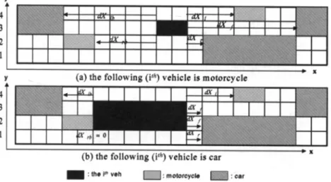
In line with the vehicle dimensions and observed minimum gaps, we define a common cell unit with much finer square grid as 1.25~1.25 meters. Thus, based on the field observation, a motorcycle in our CA models occupies 2x1 cells and a passenger car takes away 6x2 cells while moving. In addition, we consider both “car-following” and “lane-changing’’ behaviors for each particle that changes its positions over time and over a two-dimensional space, in which X-axis indicates the vehicle’s longitudinal movement distance and Y-axis denotes the vehicle’s lateral displacement distance. Each cell can be either empty or occupied at each time step. The time step in updating the related information for all particles is set as one second so that the magnitude of speed (meters per second) is exactly equal to the longitudinal position change (meters). According to the filed survey, the maximum speeds for motorcycle and car are nearly the same, thus we set both with identical maximum speed as 13 cells (about 58kph). The gaps between the following particle (either motorcycle or car) and the front, right-front, left-front, right-behind and left-behind particles, respectively denoted by are illustrated in Figure 1. In Figure l(a), the
th
following particle is a motorcycle, which uses the 3rd lateral cell lane with two motorcycles and two cars in both adjacent lanes. In Figure l(b), the ith following particle is a car, which occupies the 2”d and 3rd lateral cells with the same surrounding traffic situation. Note from Figures l(a) and l(b) that, even with exactly the same surrounding situation, the above-mentioned gaps are different because of the non-identical sizes of328
the following particles.
L. W. Lan and C-W. Chang
Y (a) the following (P) vehicle is motorcycle
I
(b) the following (irh) vehicle is car
: the I# veh : motorcycle : car
Figure 1. An illustration of inhomogeneous particles layout
2.2 Definition of CA rules
Nagel and Schreckenberg [1992] first introduced a prototype CA traffic model, which simulated single-lane (one-dimensional) pure car motions with simple updating rules. In the NaSch model, the road was divided into identical square cells of length 7.5 meters and each cell could either be empty or occupied by one car. The states of all cars at time step t + l were obtained from those at time step t by applying the given rules at the same time. In this paper, we modify the NaSch model to simulate the two-dimensional mixed traffic motions with two different types of particles. We define the CA rules that govern the particles moving logics, including moving forward and lateral displacements from left to right or the reverse. Following the previous CA lane-changing models [Rickert et al. 1996; Chowdhury et al. 1997; Nagel et al. 1998; Knospe et al. 19991, we define a particle can change its “lane” (1.25-m cell in our definition) if both of the following two criteria are satisfied.
The first one is the incentive criterion: the gap in front of particle i at the current lane should be smaller than the current speed of i and the gap in front of i in the adjacent lane(s) should be larger than the current front gap of i. The second one is the safety criterion: any lateral displacement
Inhomogeneous Cellular Automata ... 329
is possible for vehicle i only when its adjacent lane(s) is empty and the speed of the left- or right-behind vehicle is smaller than the gap between vehicle i and the behind vehicle(s). Namely, the front gap of i in the adjacent lane(s) is larger than the current speed of i; and the behind gap of i in the adjacent lane(s) is larger than the current speed of behind vehicle. In fact, the above "lane changing" rules have included both symmetric and asymmetric situations. The particle that uses the intermediate cell(s) can make a symmetric lane change from both sides depending on which side provides larger gap. However, the particle that uses the edge (right-most or left-most) cell can only make an asymmetric lane change from one side in case that the adjacent gap is large enough.
Let &f,
au'r
, dx', ,
d x t b,
d;y'rb and &rb respectively denote the gaps between vehicle i and the front, left-front, ri ht-front, behind, left-behind and right-behind vehicles at time step t; = ( X k y ' i ) ,pf
=(X>)')), P'I = (X',,.Y'l), p r = (x'r,r'r)
,
p b = (X'b,Y'b), p l b = (X 16,y'lb) and P t r b = (X'rb,$rb) respectively denote the positions of vehicle i, front, left-front, right-front, behind, left-behind and right-behind vehicles at time step t. A random enerator is used to determine the vehicles' initial= (x'lb,
O),
and v r b = (x rl,, 0) respectively denote the speed vectors of vehicle i, left-front, right-front] behind, left-behind and right-behind vehicles at time step t; Lj,Lk,
L 1, and Ltr denote the lengths of vehicle i, front, left-front and right-front vehicles at time step t; PC denote thevector of lateral position changed, in which PC = (0,-1) represents vehicle i changing to the right and PC = (0,l) changing to the left. Starting from an arbitrary initial condition with speed V o i = (Voj,O) and
Poi = (x"j,y"i) and position, the states of the particles in our CA models are updated according to the following rules:
F
positions. Let,
Vj
= (X j,o),
V l = (~ ' 1 ,o),
V r = (X'r,01,
V t b = (X'b, 0), v i bEstimate the desired speed VdeSjred and the effective gaps
dx;.,
dx:
,
Check both incentive and safety criteria;Select the largest gap; Update the speeds;
Particle i updates its speed under the following logics:
dx:
9 a b9dx',
and &rb;If
dx;-
> v ;7
then V;+' = Min
[v:
+ (1, 0 ) , ( v m a x , o ) ] .Else, if
au:
'
'i
and d x t b > ' f b ordx:
'
' i
and d x : b >'f.bv;+l
=v,!
+
PC.330 L. W. Lan and C-FY Chang
Else, cannot change lateral position,
v;+1
= @;+I, 0 ) ( 5 ) Update the positions;Particle i moves from
P,
to P?‘ based on the updated speed; namely,p;+1 = pi’
+
v;+1
3. Simulations
The initial conditions in the following simulations are set as follows.
A total of 150 inhomogeneous particles (cars and motorcycles) are
generated according to given traffic mixtures (percentages of car) from 0% to 100%. In the longitudinal direction, particles are equally spaced with distance headway (gap plus length of front particle) of 10 cells; however, in the lateral direction, particles are randomly scattered. Each particle moves at identical speed of 1 cell per second.
The aforementioned CA rules for updating the particle speeds and positions are used to simulate the particles’ movements in the road section without interruptions by curb parking, pedestrian crossing, traffic light, etc. This study attempts five cases with “lane” width of 2 cell units (2.5m), 3 cell units (3.75m), 4 cell units (5m), 5 cell units (6.25m) and 6 cell units (7.5m). In both cases I (2.5m) and I1 (3.75m), it is impossible for any car to move in parallel along with the other car, thus the car has no chance to overtake another car. In other three cases, the car may have chances to overtake another car provided that the empty cells in the adjacent space are good enough. In contrast, it is possible for a motorcycle to move in parallel along with the lateral motorcycle(s). Except for the case I, the motorcycle can also overtake the front car or move in parallel along with the car.
3.1 The eflects of lane widths and traflc mixtures
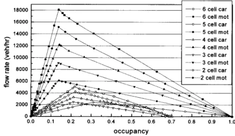
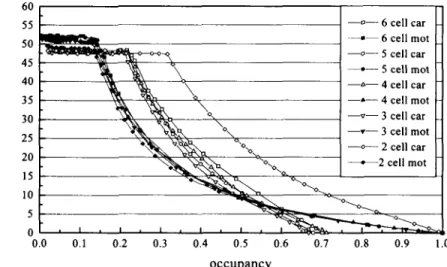
In this paper, cell occupancy (p) is used as a proxy of density, which is defined as p = N o / N, where N is the number of total cells in the study area and No is the number of occupied cells. The flow-occupancy and speed-occupancy diagrams for pure motorcycles and pure cars under various lane widths are displayed in Figures 2 and 3, respectively. We define critical occupancy (critical speed) as the cell occupancy (space-mean-speed) corresponding to the maximum flow rates. With parallel updates, the steady state is reached when the speed of each
Inhomogeneous Cellular Automata ... 331 I 18000
I\
16000 i 0.particle is the same as the speed of the front vehicle. The average speed in steady state equals the number of empty cells divided by the number of particles; hence, the average speed is inversely proportional to the cell occupancy (a proxy of density). Therefore, as the occupancies are smaller than the critical occupancy, the flow rates increase along with the increase of occupancies. However, as the occupancies go beyond the critical occupancy, the flow rates decrease gradually. Both Figures 2 and 3 show that the critical occupancies for pure motorcycles are around 0.13 to 0.18 and for pure cars are around 0.22 to 0.32. The range of critical occupancies for pure cars has concurred with the findings by Nagel [1998]. Both Figures 2 and 3 also show that the jammed occupancies for pure motorcycles can reach 1.0 in the five cases but for pure cars are only about 0.7 with an exception that case I can also reach 1.0. These phenomena are due to the fact that there is lower chance for pure cars to overtake the other particles; as a consequence, the cells utilization efficiency is less than that for pure motorcycles.
Figure 4 shows the relationship between maximum flow rates and traffic mixtures under various lane widths. Note that the maximum flow rates have a sharp decline from zero to 50 percentages of cars and a mild decline from 50 to 100 percentages in case I, implying that 50 percentages of cars could be the least cell utilization efficiency in case I.
-0- 6 cell car -=- 6 cell mot
-0- 5 cell car
14000 -0- 5 cell mot
-A- 4 cell car -A- 4 cell mot
r -v- 3 cell car a, a, -...--'-- 3 cell mot
5
8000-
2 cell car -2 cell mot6
6000 4000 2000 0 h L f 12000 2 10000 c 0.0 0.1 0.2 0.3 0.4 0.5 0.6 0.7 0.8 0.9 1.0 occupancyFigure 2. Flow-occupancy diagrams for pure motorcycles and pure
332 L. W Lan and C- W. Chang 65 60 55
=
50 y 45 -0 h-
5 cell car ---*- 5 cell mot--
4 cell car-A- 4 cell mot
-0- 3 cell car --.- 3 cell mot
-
2 cell car -2 cell mot8
40 35&
30$
25 15 10 5 0.0 0.1 0.2 0.3 0.4 0.5 0.6 0.7 0.8 0.95
20 0 1 ' ' I ' I ' ' I ' -%1 7 occupancyFigure 3. Speed-occupancy diagrams for pure motorcycles and pure cars 0 -v- 5 cell & 6 cell 20000 16000
s
v9
14000 l 8\.
O o 0 32
12000rc5
10000 - A E . . A -----
A.
- __7
v
-1 - - A 4000 2000 --e-:--..
.-
I-r--
1 . 1 . 1 . 1 . 1 . 1 . 1 . 1 . 1 . 0 10% 20% 30% 40% 50% 60% 70% 80% 90% 100%percentage of car (YO)
Inhomogeneous Cellular Automata. .. 333
Furthermore, the maximum flow rates are highly influenced by the width of lane and percentages of car. For example, under the condition of pure motorcycles, the maximum flow rates in cases I1 and V are 50% and 200% higher than that in case I. Under the condition of pure cars, in contrast, the maximum flow rates are the same in both cases I and 11, and case V is only 126% higher than both cases. The results also evidently explain that the following car cannot overtake the front car for both cases I and 11.
3.3 The motorcycle equivalents (me)
Similar to the concept of “passenger car equivalent” (pce), which represents the throughput capability of one vehicle of other types (such as bus, truck) equivalent to the maximum number of car throughputs under identical traffic and environmental conditions, we define the “motorcycle equivalent” (me) as the throughput capability of one car equivalent to the maximum number of motorcycle throughputs under identical conditions. The value of me for any two traffic mixtures under the same speed condition is defined as follows:
where PI , P2 are the percentages of cars; q1 , q2 are the flow rates corresponding to PI and P2. Note that the pce value is equal to 1/ me.
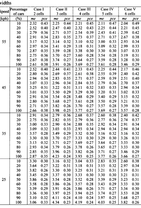
Table 1 summarizes the me and p c e values under different traffic mixtures and lane widths. In case I, for example, the me values can range from 2.32 to 2.61 (at speed 55kph) and from 3.97 to 4.00 (at speed 5kph) with respect to 10% to 100% of cars. For pure cars with speed 55kph, the
me values are from 2.61 to 3.46 as the lane width increases from two to
six cells.
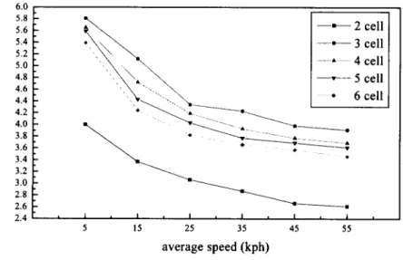
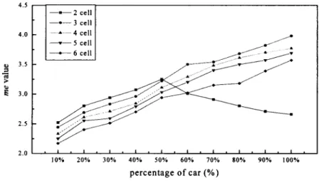
Figure 5 demonstrates the me values with respect to various speeds for pure cars. Note that the me values decrease as the speed increases in all cases. When cars get closer the average speeds would become lower; consequently, the me values should be higher. The lower me values occur in higher speeds, in which the efficiencies of cell utilization for cars and for motorcycles are nearer. Generally, the me values decrease as the lane width increases, indicating that wider roads provide higher degrees of freedom for particles’ moving and overtaking than the narrower ones do.
Figure 6 illustrates the me values with respect to different
334 L. W. Lan and C-W. Chang
values with respect to various car mixtures. It has the highest me values, the worst cells utilization efficiency, as the car percentages are lower than 50%. Nevertheless, it turns out to be the lowest me values, the best cells utilization efficiency, as the car percentages are above 60%. This interesting result reflects the fact that if motorcycles are the majority, once the cars appear, the following motorcycles would have no chance at all to overtake the cars in case I but the overtaking chance becomes higher as the lane width gets larger. In contrast, if cars become the majority in case I, the motorcycles will be grouped into several blocks by any two cars, thus makes the cell utilization better than the other cases.
6.0 5.8 5.6 5.2 5.4
1
*\\ 5 0-
4.8-
4 6-
4 4-
4 2 4 0 3 8 3 6 3 4 3.2 3 0 - 2 8 - 2.6-
2 4l
-
.
1 . I 1 , I I 1 5 15 25 35 45 55 average speed (kph)Inhomogeneous Cellular Automata ... 335
Table 1. The me and pee values under various traffic mixtures and lane widths - Speed - 55 - 45 35 25 'ercentage Case I of cars- (YO) 10 20 30 40 50 60 70 80 90 100 10 20 30 40 50 60 70 80 90 100 10 20 30 40 50 60 70 80 90 100 10 20 30 40 50 60 70 80 90 100 2 cells me pce 2.32 0.43 2.52 0.40 2.79 0.36 2.91 0.34 3.17 0.32 2.97 0.34 2.87 0.35 2.75 0.36 2.67 0.38 2.61 0.38 2.52 0.40 2.80 0.36 2.94 0.34 3.07 0.33 3.25 0.31 3.01 0.33 2.91 0.34 2.80 0.36 2.71 0.37 2.66 0.38 2.91 0.34 2.75 0.36 3.00 0.33 3.09 0.32 3.57 0.28 3.30 0.30 3.13 0.32 2.93 0.34 2.85 0.35 2.87 0.35 3.30 0.30 3.64 0.27 3.82 0.26 3.45 0.29 3.86 0.26 3.58 0.28 3.39 0.29 3.36 0.30 3.10 0.32 3.06 0.33 Case I1 3 cells me pce 2.25 0.44 2.47 0.40 2.71 0.37 2.83 0.35 3.14 0.32 3.41 0.29 3.59 0.28 3.70 0.27 3.74 0.27 3.91 0.26 2.44 0.41 2.69 0.37 2.83 0.35 2.96 0.34 3.22 0.31 3.50 0.29 3.54 0.28 3.68 0.27 3.82 0.26 3.98 0.25 2.79 0.36 2.82 0.35 2.90 0.34 3.03 0.33 3.49 0.29 3.70 0.27 3.71 0.27 3.79 0.26 3.96 0.25 4.23 0.24 3.16 0.32 3.22 0.31 3.30 0.30 3.37 0.30 3.54 0.28 3.86 0.26 3.91 0.26 3.97 0.25 4.1 1 0.24 4.34 0.23 Case I11 4 cells me pce 2.21 0.45 2.32 0.43 2.54 0.39 2.73 0.37 3.10 0.32 3.18 0.31 3.38 0.30 3.60 0.28 3.64 0.27 3.69 0.27 2.33 0.43 2.61 0.38 2.71 0.37 2.84 0.35 3.11 0.32 3.29 0.30 3.48 0.29 3.61 0.28 3.70 0.27 3.77 0.27 2.68 0.37 2.79 0.36 2.88 0.35 2.93 0.34 3.32 0.30 3.33 0.30 3.69 0.27 3.78 0.26 3.82 0.26 3.93 0.25 3.04 0.33 3.18 0.31 3.25 0.31 3.33 0.30 3.52 0.28 3.57 0.28 3.86 0.26 3.94 0.25 4.10 0.24 4.19 0.24 Case IV 5 cells me pce 2.11 0.47 2.25 0.44 2.43 0.41 2.71 0.37 3.00 0.33 3.09 0.32 3.30 0.30 3.54 0.28 3.59 0.28 3.61 0.28 2.25 0.44 2.55 0.39 2.59 0.39 2.79 0.36 3.03 0.33 3.20 0.31 3.40 0.29 3.50 0.29 3.57 0.28 3.69 0.27 2.60 0.38 2.77 0.36 2.92 0.34 2.94 0.34 3.16 0.32 3.29 0.30 3.64 0.27 3.65 0.27 3.71 0.27 3.77 0.26 2.83 0.35 3.15 0.32 3.21 0.31 3.30 0.30 3.39 0.29 3.43 0.29 3.71 0.27 3.74 0.27 3.97 0.25 4.03 0.25 Case V 6 cells me pce 2.04 0.49 2.21 0.45 2.39 0.42 2.67 0.38 2.93 0.34 2.99 0.33 3.07 0.33 3.19 0.31 3.28 0.30 3.46 0.29 2.17 0.46 2.40 0.42 2.51 0.40 2.70 0.37 2.94 0.34 3.02 0.33 3.15 0.32 3.21 0.31 3.39 0.30 3.57 0.28 2.40 0.42 2.74 0.37 2.91 0.34 2.94 0.34 3.16 0.32 3.26 0.31 3.33 0.30 3.33 0.30 3.46 0.29 3.66 0.27 2.60 0.38 2.97 0.34 3.19 0.31 3.21 0.31 3.23 0.31 3.33 0.30 3.34 0.30 3.53 0.28 3.68 0.27 3.82 0.26
336 L. W. Lan and C- W. Chang
Table 1 (continued). The me andpce values under various trafic
mixtures and lane widths
20 30 40 50 60 70 80 90 100 10 20 30 40 50 60 70 80 90 100 Speed 3.81 0.26 4.01 0.25 4.26 0.23 4.30 0.23 3.89 0.26 3.74 0.27 3.66 0.27 3.49 0.29 3.37 0.30 3.97 0.25 4.28 0.23 4.33 0.23 4.50 0.22 4.65 0.22 4.67 0.21 4.47 0.22 4.37 0.23 4.19 0.24 4.00 0.25
&!?L
15 5 Percentage I Case I1 3 cells me pce 3.43 0.29 3.80 0.26 3.94 0.25 3.41 0.29 4.21 0.24 4.29 0.23 4.80 0.21 4.91 0.20 4.97 0.20 5.12 0.20 3.86 0.26 4.00 0.25 4.15 0.24 4.31 0.23 4.54 0.22 5.05 0.20 5.42 0.18 5.52 0.18 5.60 0.18 5.81 0.17 Case I11 4 cells me pce 3.23 0.28 3.59 0.28 3.70 0.27 3.81 0.26 4.15 0.24 4.22 0.24 4.43 0.23 4.49 0.22 4.61 0.22 4.72 0.21 3.63 0.28 3.74 0.27 4.07 0.25 4.21 0.24 4.33 0.23 4.49 0.22 4.85 0.21 5.11 0.20 5.50 0.18 5.65 0.18 Case IV 5 cells me pce 3.09 0.32 3.32 0.30 3.35 0.30 3.36 0.30 3.62 0.28 3.96 0.25 4.07 0.25 4.23 0.24 4.25 0.24 4.43 0.23 3.42 0.29 3.41 0.29 3.52 0.28 3.89 0.26 4.13 0.24 4.21 0.24 4.74 0.21 4.88 0.21 5.36 0.19 5.59 0.18 Case V 6 cells me pce 2.79 0.36 3.27 0.31 3.30 0.30 3.31 0.30 3.46 0.29 3.72 0.27 3.93 0.25 4.03 0.25 4.10 0.24 4.24 0.24 3.18 0.31 3.26 0.31 3.45 0.29 3.74 0.27 3.87 0.26 4.17 0.24 4.47 0.22 4.72 0.21 4.97 0.20 5.39 0.19 4 5 -=- 2 cell -0-3 cell A ~ 4 cell 1- 5 cell - 6 cell I. 4 0-
3 5-
9, m E 3.0 -s
-
2 5 - 2 0 ' l " . l ' l ' l ' l ' l ' l ' l . l . 10% 20% 30% 40% 50% 60% 70% 80% 90% 100% percentage of car (%)Inhomogeneous Cellular Automata ... 33 7
4. Validation
In order to validate the proposed inhomogeneous CA models, we
conducted a two-hour survey (16:30 to 18:30pm) in the T-2 Provincial
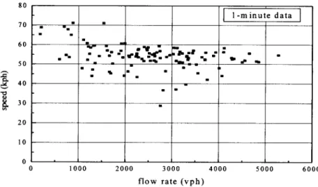
Highway at Chuwei of Taipei County. The southbound mixed traffic scenes in the outer lane of 3.5-meter width were recorded by a video camera and a total of 4,882 vehicles were observed (motorcycles are prohibited in the inner lanes). This survey has obtained 120 one-minute flow rates with corresponding speeds and densities. Figure 7 displays the speed-flow relationship for these 120 samples. Figure 8 further shows the space mean speed distributions for individual motorcycles and cars, which approximately follow normal distributions with mean 55 kph and standard deviation 1 1.8 kph.
Note from Figure 8 that the speeds for motorcycles in the T-2 Highway are slightly higher than the cars. Thus, we further undertake a statistical test and the result (X2 - 81.71 > X2(0.o~,,~, = 18.3) has rejected the null hypothesis that speed is independent of the vehicle type. Therefore, we modify the aforementioned CA parameters by assigning the car with maximum speeds of 12 cell units (54 kph) and the motorcycle with 13 cell units (58.5 kph). The field observed data in T-2
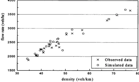
Highway and the simulated data are presented in Figure 9 and Table 3.
Note that most of the discrepancies between the observed and simulated data are less than f 5%, suggesting that our CA rules have been validated by another field observation.
flow rate ( v p h )
338 4000
z
3500 ?? E &2
v 3000 2500 2000 1500 1600 1200 o x-
x >p o x R X 0 8 O n yw ? '
90@:xx x7: 0 3 x Observed data 0 Simulated data I I 1 IL. W. Lan and C- W. Chang
0 c 400 n 0 10 20 30 40 50 60 70 80 90 100 110 120 speed (kph)
Figure 8. Observed space mean speed distributions in T-2 Highway
339
71% 70%
Inhomogeneous Cellular Automata.. .
Table 2. A comparison between observed and simulated data in T-2
54.69 2,362 43.18 56.09 2,450 43.68 3.73% 53.73 2,032 37.81 56.09 2,095 37.36 3.12% Highway 73% 79% Flow rate (%> Observed percentages of motorcvcle 56.66 2,440 43.06 56.09 2,450 43.68 0.42% 55.65 2,290 41.15 56.16 2,359 42.00 3.00% I I
Note: *speed and flow rate are measured from the observed data; density are calculated from dividing flow rate by speed.
**speed and density are measured from the simulated data; flow rate are calculated from the product of speed and density.
340 L. W. Lan and C- W. Chang
5. Stochastic CA models
One of our deterministic CA rules has set the maximum speeds for individual vehicles of the same type with a fixed value. Of course, this assumption is too strict and does not fully fit the real world situations. Therefore, we further allow the deviations of maximum speeds for individual particles by modifying the CA rules with stochastic maximum speed distributions. Take an example that the maximum speeds are normally distributed with mean 13 cells and standard deviation 1 cell,
denoted by N( 13,l). The flow-occupancy and speed-occupancy diagrams
for pure cars and pure motorcycles with stochastic maximum speeds
N(13,l) are shown in Figures 12 and 13. Compared with Figures 2 and 3
obtained from deterministic maximum speeds N (1 3,0), we find that both
maximum flow rates and critical speeds by the stochastic CA models have decreased. It is due to the “slow-vehicle” effects.
In this N(13,l) example, Figure 12 further presents the maximum flow rates with respect to various traffic mixtures. Figure 13 displays the
me values for various maximum speeds under pure car condition. Figure
14 shows the me values with respect to various traffic mixtures at speed
45 kph. Compared with Figures 6, 7 and 8 obtained from deterministic
maximum speeds N (13,0), we find that the corresponding me values for
the stochastic CA models are apparently higher. It explains that with the
variation of maximum speeds, some slow vehicles have reduced the
overall particles moving freedom.
4- 5 cell c a r ~ 5 cell mot -A- 4 cell c a r
--
3 cell c a r---
3 cell m o t 0.0 0.1 0 . 2 0.3 0.4 0.5 0.6 0.7 0.8 0.9 1.0 occupancyFigure 10. Flow-occupancy diagrams for pure motorcycles and pure cars
Inhomogeneous Cellular Automata ... 16000" 341
-.-
2 cell -0- 3 cell ' 60 55 -0- 6 cell car + c^ 14000 !? ~~ --*- 6 cell mot 50 -0- 5 cell car -0- 5 cell mot 45--
4 cell car 4035 -A- 4 cell mot
-v- 3 cell car 30 -v- 3 cell mot 25 -0- 2 cell car 20 15 10 5 0 0.0 0.1 0.2 0.3 0.4 0.5 0.6 0.7 0.8 0.9 1.0 occupancy A 4 cell -v- 5 cell Figure 11. Speed-occupancy diagrams for pure motorcycles and pure
cars
(Stochastic CA models with maximum speeds
-
N(13,l)).j 0 l2000
E
g
10000 G 8000.i
6000 -\1
+ 6 cell1
+
I 0 10% 20% 30% 40% 50% 60% 70% 80% 90% 100% percentage of car (%)Figure 12. Maximum flow rates for various traffic mixtures (Stochastic CA models with maximum speeds
-
N ( 1 3 , l ) )342 4.2 4.0 3.0 3.6 3.4
3
3.2 m 3.0 E 2.0 2.6 2.4 2.2L. W. Lan and C-W. Chang
-
- --
- 1 - --
--
6 . 0 I 5.8 5 . 6 5 . 4 5 . 2 5 .O 4 . 8 4.6 4 . 4 4.2 4 . 0 3.8 3.6 3.4 3.2 3.0 2.8 2.6 2.4 2.2 2.0 5 1 5 25 35 45 average speed (kph)Figure 13. The me values at various speeds under pure car condition (Stochastic CA models with maximum speeds
-
N (13,l))4.4 , 2 cell
--
3 cell -A- 4 cell---
5 cell 2.0 I r l , l , l , l . l r l . l . I , l . 10% 20% 30% 40% 50% 60% 70% 80% 90% 100% percentage of car (%)Figure 14. The me values for various traffic mixtures at speed 45 kph (Stochastic CA models with maximum speeds
-
N (13,l))Inhomogeneous Cellular Automata ... 343
Figures 17 and 18 fbrther compare the simulation results for pure motorcycles and pure cars among different standard deviations of maximum speeds (zero, one and two standard deviations): N (13,0), N
(13,l) and N (13,2). We find that as the maximum speed deviations get larger, the optimal speeds and maximum flow rates have significantly declined. Tables 4 and 5 present the details of maximum flow rates and optimal speeds among different maximum speed deviations. We conclude that the maximum flow rates and critical speeds are negatively influenced by the deviation of maximum speeds; but the influence is less significant as the lane width gets larger.
v-
0 m 4100 m m lmlml4100lmlm
Figure 15.
speed deviations (pure motorcycles)
344 (2.5 m (3.75 m (5 m) (6.25 m
("
7.5 mL. W. Lan and C-W. Chang
a 6,000 9,000 12,000 15,000 18,000 Figure 16.
speed deviations (pure cars)
Speed-flow diagrams of CA models with various maximum
Table 3. Maximum flow rates with various maximum speed deviations
Lane width
k
N 13,O13,400 -10.7% 12,800 -14.7% 4,150 3,520 -15.2% 2,900 -30.1% 16,250 -9.7% 15,950 -1 1.4% 5,200 4,450 -14.4% 3,650 -29.8%
Inhomogeneous Cellular Automata ... 345
Table 4. Critical speeds with various maximum speed deviations
2 cells (2.5 m) 3 cells (3.75 m) 4 cells (5 m) 5 cells (6.25 m) 6 cells (7.5 m) Pure motorcycles (kph) N(13,O) N(13, I ) N(13.2) Lane width 58.5 49.5 42.0 58.5 51.0 44.6 58.5 51.3 47.0 58.5 51.8 47.1 58.5 52.0 48.4 Pure cars (kph) N(13,O) N(I3, I ) N(13,2) 58.5 47.5 39.0 58.5 47.5 39.0 58.5 47.7 39.3 58.5 48.2 40.0 58.5 48.3 40.5 6. Concluding Remarks
Previous works on CA traffic models focused on pure cars only. Some of which defined the cell unit with a rather coarse scale, thus the particles might have unrealistic speed jumps or drops. This is obviously not consistent with what we can observe in the mixed traffic contexts. To overcome these shortcomings, we define a common cell unit with much finer square grid as 1.25~1.25 meters. Based on the field observation, a
motorcycle in our proposed CA models always occupies 2x 1 cells and a
passenger car always takes away 6x2 cells. The maximum speeds for the
motorcycle and car are of the same, which are set as 13 cell units per time step with no deviation in our deterministic CA models. The simulation results have shown reasonable interacting relationships among particles in the mixed traffic environments. To validate the deterministic CA models, we use another set of field data where maximum speeds of motorcycle and car are not the same; thus, the CA rules have been slightly modified to accommodate the distinct maximum speeds between these two vehicle types.
In line with the real world situations, we further develop stochastic CA models by considering the deviations of maximum speeds for individual particles of the same type. Compared with the deterministic CA models, we examine the effects of maximum speed deviations on the maximum flow rates and the corresponding critical speeds. It is found that both maximum flow rates and critical speeds have declined with an increase of maximum speed deviations. It is due to the slow-vehicle effect that deteriorates the cell utilization efficiency; however, such decline effect is less significant as the road (lane) gets wider.
346 L. W. Lan and C- K Chang
The present study does not mark the lane to guide the motorcyclists and car drivers, thus the vehicles may occupy the lateral cells in an inefficient manner. Marking the lanes and revising the CA rules accordingly deserve further investigation. The paper deals only with the interacting movements of two vehicle types, motorcycle and car, on the road section where flows are not interrupted by curb parking, crossing vehicles or pedestrians, traffic signals or the like. Future studies can consider more types of vehicles, such as bus and bicycle, with interruptions or traffic lights on the road section or at intersection. However, it requires introducing more complicated CA rules that can govern the particles stopping, starting, moving or turning behaviors. Special attentions must be paid to control the particles acceleration or deceleration to avoid any unrealistic abrupt speed jumps or drops. Since the motorcyclists and car drivers may act in a different way in other cities or countries, more empirical case studies from different field environments also deserve further explorations.
Acknowledgements
This paper is moderately revised from the original work [Lan and Chang, 2004al presented at the International Conference on Application of Information and Communication Technology in Transport Systems in Developing Countries, Kalutara, Sri Lanka. The research was granted by the National Science Council of ROC (NSC93-2211-E-009-033). The authors are indebted to two reviewers for giving very good suggestions to ameliorate the original paper.
References
Bham, G. H. and Benekohal, R. F., 2004. A high fidelity traffic
simulation model based on cellular automata and car-following concepts. Transportation Research 12C, 1-32.
Bierley, R. L., 1963. Investigation of an inter-vehicle spacing display. Highway Research Record 25,58-75.
Brackstone, M. and McDonald, M., 1999. Car-following: a historical review. Transportation Research 2F, 18 1 - 196.
Chakroborty, P. and Kikuchi, S., 1999. Evaluation of the general motors
based car-following models and a proposed fuzzy inference model.
Inhomogeneous Cellular Automata ... 347
Chowdhury, D., Wolf, D. E. and Schreckenberg, M., 1997.
Particle-hopping models for two-lane traffic with two kinds of
vehicles: effects of lane-changing rules. Physica 235A, 41 7-439.
Daganzo, C. F., 1994. The cell transmission model: a dynamic
representation of highway traffic consistent with the hydrodynamic theory. Transportation Research 28B, 269-287.
Daganzo, C. F., 2002a. A behavioral theory of multi-lane traffic flow. Part I: Long homogeneous freeway sections. Transportation
Research 36B, 131-158.
Daganzo, C. F., 2002b. A behavioral theory of multi-lane traffic flow. Part 11: Merges and the onset of congestion. Transportation Research Evans, L. and Rothery, R., 1977. Perceptual thresholds in car following
-
a recent comparison. Transportation Science 1 1,60-72.
Gipps, P. G., 1981. A behavioral car following model for computer simulation. Transportation Research 15B, 105-1 1 1.
Helbing, D., 2001. T&c and related selfkhiven many-particle systems.
Reviews of Modern Physics 73,1067- 1 14 1.
Herman, R., Montroll, E. W., Potts, R. B. and Rothery, R. W., 1959. Traffic dynamics: analysis of stability in car following. Operations Research 7, 86- 106.
Hermann, M. and Kerner, B. S., 1998. Local cluster effect in different
traffic flow models. Physica 255A, 163-188.
Knospe, W., Santen, L., Schadschneider, A. and Schreckenberg, M., 1999. Disorder effects in cellular automata for two-lane traffic. Physica 265A, 6 14-633.
Kometani, E. and Sasaki, T., 1959. A safety index for traffic with a linear spacing. Operations Research 7,707-720.
Krug, J. and Spohn, H., 1988. Universality classes for deterministic surface growth. Physical Review 83A, 427 1-4286.
Lan, L. W., Wang, J. C. and Chiang, C. I., 1994. On the car following model with fizzy control. Transportation Quarterly 25,43-55.
Lan, L. W. and Yeh, H. H., 2001. Car following behavior for drivers with non-identical risk aversion: ANFIS approach. Journal of the Chinese Institute of Civil & Hydraulic Engineering 13,427-434. Lan, L. W. and Chang, C. W., 2004a. Inhomogeneous particles hopping
models for mixed traffic with motorcycles and cars. International Conference on Application of Information and Communication Technology in Transport Systems in Developing Countries, Kalutara, Sri Lanka, August 5-7.
Lan, L. W. and Chang, C. W., 2004b, Motorcycle-following models of 36B, 159-169.
348 L. W. Lan and C- W. Chang
General Motors (GM) and adaptive neuro-fuzzy inference system
(ANFIS). Transportation Planning Journal 33, 51 1-536.
Lighthill, M. H. and Whitham, G. B., 1955. On kinematic waves: a theory of traffic flow on long crowed roads. Proceedings of the Royal Society, Series A 229,3 17-345.
Liu, G., Lyrintzis, A. S . , and Michalopoulus, P. G., 1998. Improved high-order model for freeway traffic flow. Transportation Research Record 1644,37-46.
May, A. D., 1990. Traffic Flow Fundamentals. Prentice-Hall Inc., New Jersey.
Michaels, R.M. and Cozan, L. W., 1963. Perceptual and field factors causing lateral displacement. Highway Research Record 25, 1
-
13.Nagel, K. and Schreckenberg, M., 1992. A cellular automaton model for freeway traffic. Journal de Physique I France 2,222 1-2229.
Nagel, K., 1996. Particle-hopping models and traffic flow theory.
Physical Review 53E, 4655-4672.
Nagel, K., 1998. From particle-hopping models to traffic flow theory.
Transportation Research Record, 1644, 1-9.
Nagel, K., Wolf, D. E., Wagner, P. and Simon, P., 1998. Two-lane traffic
rules for cellular automata: A systematic approach. Physical Review
Payne, H. J., 1971. Model of &way traf€ic and control. Mathematics of
Public Systems 1,51-61.
Pipes, L. A., 1967. Car following models and the fundamental diagram of road traffic. Transportation Research Record 1 , 2 1-29.
Pottmeier, A., Barlovic, R., Knospe, W. and Schadschneider, A., 2002.
Localized defects in a cellular automaton model for traffic flow with phase separation. Physica 308A, 47 1-482.
Richards, P. I., 1956. Shock waves on highway. Operations Research 4,
Rickert, M., Nagel, K., Schreckenberg, M. and Latour, A., 1996. Two
lane traffic simulation using cellular automata. Physica 23 1 A, Rockwell, T. H. and Treiterer, J., 1968. Sensing and communication
between vehicles. NCHRP Report 5 1, HRB, Washington, D.C. Wang, B. H., Wang, L., Hui, P. M. and Hu, B., 2000. The asymptotic
steady states of deterministic one-dimensioned traffic flow models. Physica 27B, 237-239.
Wei, C. H. and Lin, H. C., 1999. Construction of car-following models
using artificial neural networks and genetic algorithms.
Transportation Planning Journal 28,353-378.
58E, 1425-1437.
42-5 1 .
Inhomogeneous Cellular Automata.. . 349
Wolf, D. E., 1999. Cellular automata for traffic simulations. Physica Wolfram, S., 1986. Theory and Applications of Cellular Automata. Word
Scientific, Singapore.
Wong, G . C. K. and Wong, S. C., 2002. A multi-class traffic flow model - an extension of
L W R
model with heterogeneous drivers. Transportation Research 36A, 827-841.Zhang, H. M., 1998. A theory of nonequilibrium traffic flow.
Transportation Research 32B, 485-498. 263A, 438-45 1.