規則導向式動態投資組合保險決策輔助模型之建構

全文

(1)國立交通大學資訊管理研究所博士論文. 規則導向式動態投資組合保險決策輔助模型之建構 Construction of Rule-Oriented Decision Support Models for Dynamic Portfolio Insurance. 研究生：陳美支指導教授：陳安斌. 博士. 中華民國九十七年四月.

(2) 規則導向式動態投資組合保險決策輔助模型之建構 Construction of Rule-Oriented Decision Support Models for Dynamic Portfolio Insurance. 研究生：陳美支. Student：Mei-Chih Chen. 指導教授：陳安斌. Advisor：An-Pin Chen. 國立交通大學資訊管理研究所博士論文. A Dissertation Submitted to Institute of Information Management College of Management National Chiao Tung University in Partial Fulfillment of the Requirements for the Degree of Doctor of Philosophy in Information Management. April 2008 Hsinchu, Taiwan, the Republic of China. 中華民國九十七年四月.

(3) 規則導向式動態投資組合保險決策輔助模型之建構. 學生：陳美支. 指導教授：陳安斌. 國立交通大學資訊管理研究所博士班. 摘. 要. 現今的投資環境複雜且多變，金融市場經常受許多因素的影響而瞬息萬變，不論對於一般的投資者或機構專業理財者而言都難以掌握其變化趨勢，本研究嘗試以時間不變性投資組合保險策略（Time Invariant Portfolio Protection，簡稱 TIPP）為基礎，採用演化式演算法（Evolution Algorithms，簡稱 EA）建構輔助決策模型，以協助投資者降低投資風險，避免鉅額損失。投資組合保險（Portfolio Insurance）是保本投資策略的一種，其概念是藉由付出少許的保險費用，以鎖定整個市場價格下跌時之風險，將損失控制於一定範圍之內，而市場上漲時卻又不失參與獲利機會。時間不變性投資組合保險策略是投資組合保險常用的策略之一，其中風險乘數（Multiple）及最低交易調整門檻值（Tolerance）是此策略的重要參數，全憑投資者經驗與喜好而設定，然而行為財務學者發現因為框架效應（Framing Effect）所致，投資者經常表現出過度反應或反應不足，因此無法根據市場變動設定適合的參數進行投資。本研究以演化式演算法動態調整風險乘數及最低交易調整門檻值並進行了兩階段式實證研究。實證結果顯示本研究所提之輔助決策模型確實可以尋得有效的參數，其模擬投資結果比傳統的 TIPP 策略及買入持有等策略表現更佳，顯示出本研究建議之模型是更保守且安全的投資組合保險模型。關鍵字：基因演算法、分類元系統、時間不變性投資組合保險、動態投資組合保險、框架效應. -i-.

(4) Construction of Rule-Oriented Decision Support Models for Dynamic Portfolio Insurance student：Mei-Chih Chen. Advisor：Dr. An-Pin Chen. Institute of Information Management National Chiao Tung University. ABSTRACT. Today‘s investment environment is complex and volatile, with numerous factors influencing the financial markets. It is difficult for individual and institutional investors to stay abreast rapid changes in this environment. This study attempts to investigate decision support models using evolution algorithms （EA）to explore the Time Invariant Portfolio Protection（TIPP） policy. Portfolio insurance is a principal-protected strategy that limits the investment portfolio losses to within a certain range when market prices decline, but also allows the portfolios to participate in profits when the market rises. Although Multiplier and Tolerance, concerned as the important parameters of TIPP, can be set up according to the individual's experiences and preferences, but scholars of behavioral finance have discovered that the investors tend to over- or under-react due to framing effect. Therefore, it is difficult for the investors to find out adequate parameters. The proposed models using evolution algorithms dynamically optimizes Multiplier and Tolerance parameters and two-stage experiments are conducted with the proposed models. The evaluation revealed that the evolutionary approaches dynamically identified satisfactory Multiplier and Tolerance parameters. The empirical results also suggested that the proposed models more conservative and safer than the buy-and-hold model and the conventional TIPP model. Keywords：Genetic Algorithms, Classifier Systems, Time Invariant Portfolio Protection, Dynamic Portfolio Insurance, Framing Effect. ii.

(5) 誌. 謝. 六年前有緣重返校園，進入交通大學學術殿堂繼續深造，是個人莫大的榮幸，走過二千多個日子，終於築夢成真，感謝交通大學及資訊管理研究所讓我在人生旅程中增添一段難忘的經歷。首先，要感謝指導老師陳安斌教授在研究上的啟發與鞭策，不論放假與否總是陪著 APC lab 的同學們奮鬥到深夜，本人謹致上最誠摯的感謝之意。此外要特別感謝碩士班學弟黃銘嘉和林昶立，因為你們的幫忙才得以讓我順利完成學業，以及一同奮鬥的博士班同學們，彼此的勉勵與協助讓我有信心繼續走下去，同時也要感謝 APC lab 的其他夥伴們，缺少您們的幫忙，我就無法實現夢想。此外，還有一群明新的同事兼好友們，沒有你們的一路加油打氣和隨時提供協助，我無法順利走完全程。最後，謹將學位獻給我的家人及親朋好友們，因為大家的支持與關懷才能讓我順利完成博士學業，這份榮耀是屬於大家的。. 陳美支謹謝. -iii-.

(6) Contents Abstract(in Chinese) …………………………………………………..…… Abstract(in English) ……………………………………………………..… Acknowledgements ……………………………………………………..… Contents …………………………………………………….……………... List of Tables ……………………………………………………………… List of Figures ……………………………………………………………… Chapter 1 Introduction……………………………………………………… 1.1 Motivation………………………………………………………… 1.2 Problem Description ……………………………………………… 1.3 Research Purpose ………………………………………………… 1.4 Dissertation Organization…………………………………………. Chapter 2 Literature Review ………………………………………….……. 2.1 Portfolio Insurance …………………………………………..…… 2.1.1 Constant Portion Portfolio Insurance …………………………… 2.1.2 Buy-and-hold Strategy ………………………………….…….… 2.1.3 Constant-mix Strategy ………………………………………..… 2.1.4 Stop-loss Strategy ……………………………………………… 2.1.5 Time Invariant Portfolio Protection……………………………… 2.2 Behavioral Finance ………………………………………….……. 2.3 Evolution Algorithms…………………………………………..…. 2.3.1 Genetic Algorithms……………………………………………… 2.3.2 Learning Classifier Systems……………………………………... 2.4 Technical Analysis ……………………………………………….. 2.5 Summary …………………………………………………………. Chapter 3 Design of Decision Support Models ………………..…………… 3.1 Research Framework …………………………………………….. 3.2 GA-based TIPP Models ………………………………………….. 3.3 XCS-based TIPP Models ………………………………………… 3.3.1 Data Preprocessing ……………………………………………… 3.3.2 Use of Genetic Algorithms ……………………………………… 3.3.3 Design of Classifier Condition Portion …….…………………… 3.3.4 Design of Classifier Action Portion …………………………...... 3.3.5 Initialization of The Rule Database …………………………....... 3.3.6 Knowledge-Rule Model ………………………………………… Chapter 4 Experiments Design and Results Analysis ………………..…….. 4.1 GA-based Experiments Design …………………………………... 4.1.1 Experimental Data ………………………………………………. 4.1.2 Parameters Setting ………………………………………………. 4.1.3 Results and Analysis ……………………………………………. 4.2 XCS-based Experiments Design …………………………………. 4.2.1 Experimental Data ……………………………………………….. -iv-. i ii iii iv vi vii 1 1 3 6 9 10 10 11 11 12 12 13 14 15 15 17 20 21 23 23 26 28 31 31 34 36 37 37 39 39 39 40 40 51 51.

(7) 4.2.2 Parameters Setting ………………………………………………. 4.2.3 Results and Analysis ……………………………………………. Chapter 5 Conclusion and Future Works ………………………………….. 5.1 Conclusion ……………………………………………………….. 5.2 Future Works …………………………………………………….. References ………………………………………………………………….. -v-. 51 53 56 56 57 59.

(8) List of Tables Table 3-1. Table 3-2. Table 3-3. Table 4-1. Table 4-2. Table 4-3. Table 4-4. Table 4-5. Table 4-6. Table 4-7 Table 4-8. Table 4-9. Table 4-10. Table 4-11.. Classifier composition.................................................................. Classifier condition portions........................................................ Composition of classifier action portions..................................... Comparative from 1996/09 to 1997/07........................................ Comparative from 2000/01 to 2000/11........................................ Comparative from 2004/07 to 2005/08........................................ Comparative of B&H, TIPP, GA-based models.......................... Comparative of B&H, Contingent, TIPP, GA-based Models...... Comparative of 70% insured from 1997 to 2007......................... Comparative of 80% insured from 1997 to 2007......................... Comparative of 90% insured from 1997 to 2007......................... Comparative of 70% insured XCS-based and GA-based models Comparative of 80% insured XCS-based and GA-based models Comparative of XCS-KRTIPP model and GA-TIPP model......... -vi-. 35 35 37 43 43 43 45 46 47 48 49 53 54 54.

(9) List of Figures Figure 1-1. Dow Jones Industrial Average of “Black Monday”..................... Figure 1-2. Floor of TIPP versus Floor of CPPI............................................. Figure 1-3. ROI Probability distribution of TIPP........................................... Figure 1-4. Research Flowchart...................................................................... Figure 2-1. A summary of a general Genetic Algorithm................................ Figure 2-2. Operation diagram of extended classifier systems....................... Figure 3-1. Research architecture................................................................... Figure 3-2. Principal Protected Investment Cycle.......................................... Figure 3-3. Example of portfolio insurance adjustment.................................. Figure 3-4. XCS-based TIPP model................................................................ Figure 3-5. Prediction model........................................................................... Figure 4-1. GA-based experiments................................................................. Figure 4-2. TAIEX from 1996/09 to 1997/07................................................. Figure 4-3. TAIEX from 2000/01 to 2000/11................................................. Figure 4-4. TAIEX from 2004/07 to 2005/08................................................. Figure 4-5. Floor of 80% insured GA-DTIPP model ( 1996/09~1997/07)..... Figure 4-6. Floor of 80% insured GA-DTIPP model ( 2000/01~2000/11).... Figure 4-7 Floor of 80% insured GA-DTIPP model ( 2004/07~ 2005/08).... Figure 4-8. TAIEX from 1989/06/22 to 1989/10/14...................................... Figure 4-9. TAIEX from 2005/01/06 to 2005/11/10...................................... Figure 4-10. 70% insured return on invest from 2004/07 to 2005/08............... Figure 4-11. 80% insured return on invest from 2004/07 to 2005/08............... Figure 4-12. 90% insured return on invest from 2004/07 to 2005/08................ -vii-. 4 5 7 9 16 18 23 24 25 30 30 40 41 42 42 44 44 44 45 46 47 48 49.

(10) Chapter 1 Introduction The purpose of this study is to construct decision support models for dynamic portfolio insurance. First, this chapter introduces the research motivation and the problem we want to solve. Then, it explains our research purpose and the organization of this dissertation.. 1.1 Motivation Today’s investment environment is complex and volatile,. with numerous factors. influencing the financial market. It is hard for individual and institutional investors to stay abreast rapid changes in the environment. It is therefore difficult to obtain steady profits from the financial market. The risks faced by investors can be classified as systematic and non-systematic risks. Non-systematic risks can be dispersed through the investment portfolios, while systematic risks cannot be avoided this way. Instead, systematic risks must be avoided through some types of portfolio insurance. The essential concept behind portfolio insurance is to pay a relatively small amount of insurance in order to obtain protection for one's underlying investment portfolio. The main goal of portfolio insurance is to eliminate or avoid all risk factors that may cause investment loss. A number of approaches can be used to protect principal, including futures hedging, options hedging, stop-loss approach, and so on. Apart from passively avoiding risk, portfolio insurance can also actively pursue returns [8]. Investors are inevitably more interested in protecting their wealth than increasing wealth during times of economic downturn. Portfolio insurance seeks to avoid excessive losses due to large-scale market fluctuations, without losing opportunities for returns when the market rises. Portfolio insurance also constitutes a dynamic asset allocation strategy. For example, the type of principal guaranteed fund that was popular in Taiwan in recent years mainly invested in fixed income financial commodities such as government bonds, treasury bills, corporate 1.

(11) bonds, ordinary CDs, and securitized asset products. When the fund comes to maturity, this amounts invested in fixed income financial commodities is roughly equivalent to the initially invested principal. In addition, another small amount is selectively invested in stocks, derivatives such as highly-leveraged futures and options, or foreign exchange in order to obtain the market profit during the investment period. This type of fund protects the investor's principal while it also provides the investor an opportunity to participate in the rises and falls of the stock market.. And so, portfolio insurance, which had been used overseas as an asset. allocation strategy for many years, are especially useful for this type of professional fund manager. In addition, individual investors with large amounts, government pension fund managers, insurance company public funds, and various types of trust funds, can also select one portfolio insurance strategy and perform assets allocation with reference to the characteristics of their funds in order to obtain maximum returns with limited risk. Taiwan's securities companies have gradually adopted this mechanism in recent years in order to ensure their assets decrease never below a guaranteed amount due to the drops of stock market. Modern financial economics assume that investors behave with extreme rationality. Rational investors trade only when the expected gains exceed transaction costs. But Brad and Terrance [23] provide strong experiments support for the behavioral finance model. The manager of the principal guaranteed fund depends entirely on personal experience in allocating funds and trading. Behavioral finance researches [22] found that Individuals and mutual funds have similar turnover rates. Individual investors and even professional fund managers allow their emotions to get in the way of rational investment decision-making [62]. Behavioral finance focuses upon how investors interpret and act on the information to make investment decisions [36]. Furthermore, it releases the traditional assumptions of financial economics and varies human departures from rationality into standard models of financial markets [23]. The financial market is a complex and continuously changing environment. Odean [64] found that the stocks individuals subsequently bought, they almost underperform 2.

(12) what they have sold. They also found that the more people traded, the worse they did [23]. Furthermore, the framing effect of the prospect theory [27] proposed that risk aversion choice is preferred in a gain situation whereas the risk seeking choice is preferred in a loss situation. Stock market investment requires decision-making in an uncertain situation. The framing effect is considered a very important psychological bias in the study of behavioral finance. This effect referring to that spot under bounded knowledge, the ordinary investors are invariably direct reactions to the received information the reality behind which they are unable to scrutinize [53].. Therefore, a portfolio insurance decision support model is needed. to prevent investors from over- or under-reaction, and help investors control downside risk and enhance investment return.. 1.2 Problem Description Portfolio insurance strategies can be classified into two types depending on trading methods. One type is based on options and is usually termed as an option-based portfolio insurance (OBPI). This strategy uses the Black-Scholes option pricing model to calculate option premiums needed by the investment portfolio, such as for European protective puts and European fiduciary call. When there is no options market, the options replication methods such as synthetic put option [51] can be used as insurance. The other type of portfolio insurance strategy involves the setting of certain parameters to provide insurance reflecting the investor's risk preferences. Examples include constant portion portfolio insurance (CPPI), time invariant portfolio protection (TIPP), constant mix strategy, and so forth. Yang and Liu [66] completed experiments which employed constant portion portfolio insurance (CPPI) and synthetic protective put (SPP) in Taiwan’s stock market from February, 1990 to October, 1990 and found that CPPI outperforms SPP strategy. They both are better than the strategy without insurance program. The researchers [68] also found that when the stock market continues to rise, OBPI strategy’s performance is stronger than CPPI strategy’s 3.

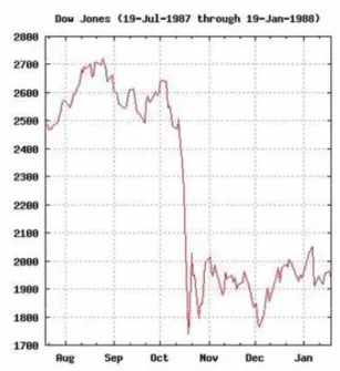
(13) performance; meanwhile, in other market conditions, CPPI strategy is better than OBPI strategy. The OBPI approaches are calendar-time dependent. A drawback of the OBPI strategy is that the long-term investors whose horizon is usually beyond the horizon specified in this strategy. In addition, the asset mix just experied is possible vastly different the mix as reset just after expiration because this approach is sensible to circumstances change. Consequently, one must utilize a relatively complex option pricing formula to find a set of rules when the strategy expires at the horizon [18].. Figure 1-1. Dow Jones Industrial Average of “Black Monday”. On October 19, 1987, a date known as “Black Monday,” the Dow Jones Industrial Index plummeted 508 points as shown in Figure 1-1(http://en.wikipedia.org). The S&P 500 dropped 20.4%. The Brady Commission Report [54] imputes the market crash to the mechanism of portfolio insurance strategy. The stock market volatility increases accompanying the increasing portion of CPPI insurers [20, 33]. Nietert [21] presents that portfolio insurance cannot protect minimum investment goals because it overlooks a real world phenomenon – “model uncertainty”. However, Nietert suggests that a more 4.

(14) sophisticated strategy is possible with CPPI. Rubinstein [50] examines “Black Monday” and suggests portfolio insurance should modify the buying strategy, while the remaining dynamic strategy should be unchanged. Moreover he also proposes conservative programs are probably outperform more aggressive programs. Time invariant portfolio protection is a derivative of CPPI. As shown in Figure 1-2, the black line represents the floor of CPPI and the blue line is floor of TIPP. TIPP not only protects principal but also locks in profits, it is more conservative than CPPI strategy.. Figure 1-2. Floor of TIPP versus Floor of CPPI Financial researchers traditionally use statistical methods to establish models for forecasting financial market trends. Decision support system must have an ability to process both quantitative and qualitative data and use reasoning to transform data into opinions, judgments, evaluations and advice. Statistical techniques have rarely been used to build intelligent support system in fields that have weak domain models [41]. In recent years, more sophisticated computer techniques have been applied to analyze financial problems [15, 16, 19, 31, 32, 39, 42, 47]. Artificial intelligence techniques have been used most frequently. 5.

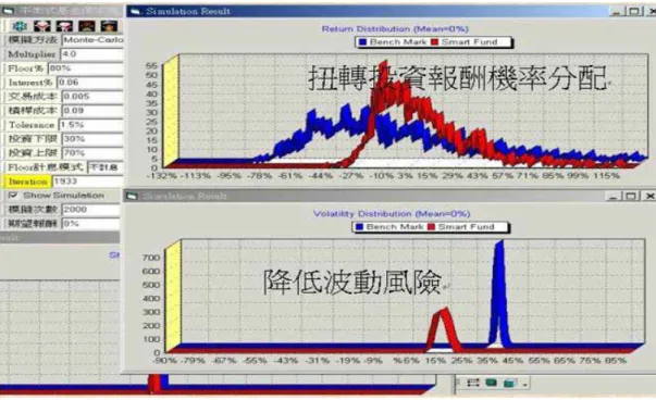
(15) Artificial intelligence methods include neural networks, decision trees, genetic algorithms, and so on. What these methods have in common is the use of large quantities of historical data to generate forecasting models through repeated learning and training. Nevertheless, the models established using conventional artificial intelligence and statistical methods [14] all constitute static models. When a static model is used to predict the future in an environment that will change, the model certainly cannot provide appropriate solutions when current phenomena are completely different from that of the training period. In view of the fact that the financial market is a dynamic environment, this research has consequently employed evolutionary algorithms and based TIPP to develop dynamic decision support models to perform asset allocation and invest with insurance for investors.. 1.3 Research Purpose The Black-Scholes formulas assume that the volatility of the underlying asset remains constant over the option’s horizon. This is not a realistic assumption [8]. Some researchers discovered that only when the stock market keeps rising, OBPI strategies outperform the CPPI strategies; however, in other stock market scenarios, OBPI was not as good as CPPI [66, 68]. After “Black Monday,” the researcher still proposes a more sophisticated insurance strategy with CPPI that is possible [21]. In addition, parameter-setting programs have the advantage of no fixed expiration date. The program can be left for as long as clients wish [8]. Therefore, this research is focused on the second type of portfolio insurance strategies and base on TIPP to develop a dynamic portfolio insurance model. TIPP [65] is mainly a modification of the CPPI strategy. CPPI employs a fixed insured principal amount, while TIPP takes the greatest of the original insured amount and the current floor. Thus, the floor will only rise and will not fall, which makes a very conservative portfolio insurance strategy. In Figure 1-3, we can also discover that the ROI probability distribution is no longer a normal distribution, the probability of loss is less than 27% and the 6.

(16) volatile is lower than the bench market. On the other hand, because parameters are set up according to the investors’ preferences, this type of insurance strategy may not achieve the protection of principal. For instance, setting the Multiplier parameter too high may cause excessive risk, and setting the Tolerance parameters too low may cause over trading and poor returns [2]. For this reason, to find out the adequate Multiplier and Tolerance parameters is the main purpose of our research.. Figure 1-3. ROI Probability distribution of TIPP. Although “time invariant” is part of the TIPP designation, its performance is connected to the time of initial investment. According to the findings of Choice and Seff [43] using the S&P 500 as an example, the rates of return on TIPP strategies from 1986 until 1987 and only invested in 1987 would be 3.6% and 13.45% respectively. This extreme disparity in rates of return shows clearly that TIPP strategies are connected to time. Many empirical studies from the last few years have shown that stock market behavior possesses certain characteristics and is predictable [17]. In view of the time-dependence of TIPP strategies and the predictability of 7.

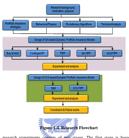
(17) stock market behavior, this study attempts to use an evolution-based TIPP strategy to construct dynamic portfolio insurance strategy models. In the insured investment process, forecasts of future stock market trends will help fund managers dynamically adjust their trading and find appropriate Multiplier and Tolerance parameters for the TIPP strategy. Finally, this study uses Sharpe ratio and rates of return on investment as performance assessment standard, and compares the evolutionary TIPP model with the buy-and-hold model and the conventional TIPP strategy model. Although the opening of Taiwan's financial markets in recent years has led to the gradual diversification of commodities, the benefits of most investors and suppliers were damaged due to “Information Asymmetry”. Ordinary investors are usually concerned about how to take advantage of market opportunities, but have no ideas to protect their principal in decline market. Generally investment management consists of three phases which are strategic asset allocation, tactical asset allocation, and stock picking [10]. Strategic asset allocation is a long-term allocation strategy to assemble an asset level allocation after evaluating the risks of each asset class and considering the investor’s preferences. Tactical asset allocation is a short-term allocation, which regularly adjusts the portfolio according to the market timing. Overall, stock selection is the most time-consuming stage [10] and has a greater impact on the return of portfolio [25]. Therefore, our study is focused on the market timing in order to select the optimal parameters under the insured period. The criticism of portfolio insurance is that it reduces return as well as reducing risk. But Leland and Rubinstein [8] describe that portfolio insurance can be used aggressively rather than simply to reduce risk when insurance program is applied to more aggressive active assets. For that reason, our research models are aggressive to maximize return and keep downside risk under controlled. Our research flowchart is as shown in Figure 1-4.. 8.

(18) Figure 1-4. Research Flowchart This research experiments consists of two stages. The first stage is based on GA construction decision support models by proving the result analysis absorbed from the experiments. The second stage is based on the learning classifier systems (LCS) and also faces to the input factors of technical indicators as to complete the construction, provement, and result analysis.. 1.4 Dissertation Organization The dissertation contains Chapter I , an introduction explaining research motivation and goals; Chapter II, a review of. the literature concerning portfolio insurance, evolution. algorithms, behavioral finance, and technical analysis; Chapter III, an explanation of the research model’s design; Chapter IV, the experiment’s design and results analysis; and Chapter V, the conclusion of the study and direction of future research. 9.

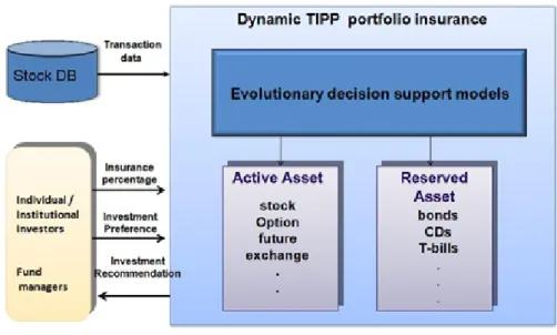
(19) Chapter 2 Literature Review This chapter examines that the previous research concerning relevant issues, including portfolio insurance strategies, behavioral finance, evolutionary algorithms, and technical analysis. The portfolio insurance strategies are at first reviewed to setup the background knowledge for developing our novel decision support models. The rest are reviewed subsequently.. 2.1 Portfolio Insurance The earliest portfolio insurance was introduced in 1956 in Britain when a commercial organization sold insurance to investors to protect their investment from possible losses. The initial financial product is known as portfolio insurance in the US was introduced in 1976; at that time the two insurance companies Harleysville and Prudential provided investment insurance to individual investors. Portfolio insurance strategies consist of asset allocation. Generally asset is classified two kinds as active assets (also known as risky assets) and reserved assets (also known as non-risky assets). Active assets constitute the high-risk, high-return assets. In contrast, reserved assets are relatively a low risk. The two types of assets are allocated on the basis of their relative risk. For instance, assets may be allocated as stocks and bonds; in this case stocks are the active assets and bonds are the reserved assets. If assets are consisted of stocks and futures; futures are the active assets and stocks are the reserved assets. Fluctuations in risky asset will cause the value of portfolio to change. Thus, dynamic strategies must decide how to rebalance the portfolio in response to such changes [18]. The following is going to review parameter-setting portfolio insurance strategies.. 10.

(20) 2.1.1 Constant Portion Portfolio Insurance The constant portion portfolio insurance [30] strategy uses simple parameter settings to achieve the goal of constant portion principal protection. This type of portfolio insurance can be expressed as the following equations (1) (2): c= A – Floor. (1). e = M*c. (2). Where: e : Exposure (amount in active assets) c : Cushion (portfolio value minus Floor) M : Multiplier A : Total value of assets Floor : the lowest insured value for the portfolio and T : Tolerance (Percentage move that triggers a trade) In the simple terms, this insurance strategy involves the setting of insurance ratio, Multiplier and Tolerance parameters reflecting the greatest risk that investors can tolerate. Risky asset position is constantly monitored throughout the investment process. Trading is implemented whenever risky asset position exceeds the Tolerance level, and total assets are recalculated. As a result, when total assets are varying during the investment period, the insured amount (Floor) does not change throughout the investment period. CPPI strategy sells stocks as the market fall and buys stocks as the market rise. Such a strategy, the portfolio might be worse than the Floor if the market drops precipitously before the investors have the chance to rebalance [18].. 2.1.2 Buy-and-hold Strategy This strategy is a “do-nothing” solution [18]. In investment period, rebalancing will not 11.

(21) be performed until exits the market. For instance, we put 70% in stock and 30% in cash. No matter what happens, no rebalancing is done. Finally, we calculate the return at the end of investment period.. Buy-and-hold is a type of CPPI strategy with Multiplier which equals to. one and a Floor equals to the value invested in bills. Some features of this strategy [18] are the portfolio value is linearly related to the stock market, the portfolio value will never fall below the value of investment in bills, and upside return potential is unlimited. As a result, the greater the initial percentage invested in stocks, the better the performance when the market is raise.. 2.1.3 Constant-mix Strategy This strategy sets a constant proportion of the portfolio to be invested in risky asset. When asset values change, the investors have to do rebalance in order to revert the fixed proportion. The constant-mix strategy is a special case of CPPI strategy which has a zero Floor and Multiplier with value between zero and one. In raise market, this strategy is constantly selling stock, and vice versa. Perold and Sharpe [18] described that whether the stock market is up or down, the buy-and-hold strategy dominates the constant-mix strategy, nevertheless the stock market is reversing itself, the constant-mix strategy capitalizes on reversals. Therefore, a constant-mix strategy outperforms the buy-and-hold strategy in a flat market and greater volatility will accentuate this effect.. 2.1.4 Stop-loss Strategy In this strategy, a downside threshold is setting at the beginning. All the assets are invested in an equity portfolio. When the asset value falls to the setting-threshold, the risky assets are exchanged for risk-free asset. This strategy always ensures the floor. But after then, if the price raises, stop-loss strategy is impossible take part in to get the profit gain. There are also a modified version of stop-loss approach be proposed [59]. The modified stop-loss 12.

(22) strategy is more gradual movement of funds from stock market to bills. After simulation, Ron , et al.[59] discovered that both the stop-loss and modified stop-loss strategies perform worse than most of synthetic puts in terms of their ability to protect against negative returns over the insured period.. 2.1.5 Time Invariant Portfolio Protection The TIPP [65] strategy chiefly amends the characteristic of the CPPI strategy that the insured amount (Floor) does not change with fluctuation of assets. CPPI and TIPP dynamically adjust active and reserved assets in the investment portfolio in order to achieve the goal of portfolio insurance. The main difference between these two strategies is that the Floor remains unchanged in the CPPI strategy. The TIPP strategy, at adjustment times, takes the larger of the amount of current asset insured percentage (A*λ, which is the current Floor) and the previous insured amount (previous Floor). As a result, the Floor can only rise, it never falls to lock that the investment profits. The TIPP strategy can be expressed as the following equation: e =M* (At ﹣Ft). (3). Ft+1 =max(Ft, At+1*λ). (4). t : adjustment time points λ : insured percentage Since the TIPP strategy based on the investor's current wealth, and it does not on a past wealth, the required insured amount gradually increases with growing wealth during the investment period. Even when the opposite situation occurs, and wealth decreases, the insured amount can never less than the previous Floor. As a consequence, TIPP is a highly conservative portfolio insurance strategy, and is therefore also referred as a dynamic double principle protection insurance strategy. Dynamic portfolio insurance strategies require constant and continuous adjustment in 13.

(23) order to achieve their theoretical effectiveness [29]. Generally speaking, commonly used adjustment methods include the fixed-time adjustment method, market fluctuation adjustment method, gap adjustment method, technical analysis adjustment method, and risk preference adjustment method. But when continuous adjustments are made, trading costs will dramatically erode investment performance [58], and portfolio insurance performance will be less than ideal when the market is fluctuating. When a bull market prevails, portfolio insurance will cause opportunity cost losses [24], but portfolio insurance will be effective to protect active asset from losing in a bearish market. When the market is fluctuating, it can’t perform well because transaction cost will affect the return.. 2.2 Behavioral Finance Efficient Market Hypothesis (EMH) has dominated financial market more than 3 decades. Nevertheless, many empirical anomalies, e.g., price earning ratio effect, size effect, intraday effect, overnight effect, weekend effect, January effect and etc., have been discovered that invalidate efficient Market Hypothesis. Arthur [67] indicated ”As the situation is replayed regularly, we look for the patterns, and we use these to construct temporary expectation models or hypothesis to work with. ” Kahneman and Tversky wanted to build a parsimonious theory to fit a number of violations of classical rationality that they had uncovered in empirical work. Expected utility theory which concerns with “how” uncertainty decision should be made, but Prospect Theory concerns with “how” decisions are actually made. Expected utility theory says that the expected utility is the sum of the probability weighted outcomes measured in terms of utility as formula (5).. ∑ P U(x t. t. (5). ). Prospect Theory thought the weights are not the true probability, and the utilities are. 14.

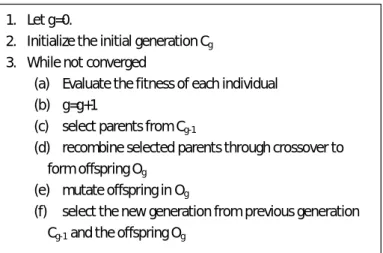
(24) determined by a value function as formula (6) rather than a utility function :. ∑ π (P )V(x t. t. (6). - r). Where π is non-linear weighting function, r is the reference point which is value function to be evaluated. For example, people are not looking at the levels of final wealth they can attain but also gain and loss relative to some reference points, which may vary from situation to situation, and display a loss aversion [3]. Prospect Theory is a descriptive theory of choice under uncertainty. There are many patterns about cognitive biases. For instance, there are certainty effect, overconfidence, framing, mental accounting, isolation etc. A behavioral finance research Ritter [38] also found Overconfidence, framing effect, and mental accounting, three common effects affecting investment decisions. People often predict future uncertain events by taking a short history of data and asking what broader picture history is representative. They often do not pay enough attention to the possibility that the recent history is generated by chance rather than by the “model” they are constructing.. 2.3 Evolutionary Algorithms Evolutionary algorithms simulate the model of natural evolution. The basic idea of evolutionary algorithms is survival of the fittest, the weak was die. Subsequently we overview two well known evolutionary algorithms: genetic algorithms and learning classifier systems.. 2.3.1 Genetic Algorithms Genetic Algorithms are evolutionary search algorithms that simulate the basic principles of natural evolution such as selection, inheritance, mutation, and population dynamics. The basic concepts of GA’s are introduced by Holland [7]. GA’s have been 15.

(25) successfully applied to various domains, such as electrical devices [37, 55], pattern recognition [70], business [28,78, 79], parameters optimization [26, 74, 75] and performed the best on various evolutionary algorithms [69]. Genetic algorithms are global optimization techniques that avoid many of the shortcomings exhibited by local search techniques on different search spaces [40]. In addition, Grefenstete showed that the standard GA, GAs outperform several classical optimization techniques on task environment. Therefore, a genetic algorithm based parameter optimization approach is proposed in the first stage of this study. The pseudo codes ( see Figure 2-1) is a summary of a general Genetic Algorithm [4].. 1. Let g=0. 2. Initialize the initial generation Cg 3. While not converged (a) Evaluate the fitness of each individual (b) g=g+1 (c) select parents from Cg-1 (d) recombine selected parents through crossover to form offspring Og (e) mutate offspring in Og (f). select the new generation from previous generation Cg-1 and the offspring Og. Figure 2-1. A summary of a general Genetic Algorithm Genetic algorithms model genetic evolution. The characteristics of individuals are therefore expressed by using genotypes. Financial markets are dynamic environments, and investors invariably to find it’s difficult by judging the state of the investment environment. Under such circumstances, Genetic algorithms can provide suitable solutions to questions. Genetic algorithms have the following basic operating procedures [13]: Step 0: initialize population. Step 1: evaluate（compute fitness） Step 2: select 16.

(26) Step 3: crossover Step 4: mutate Step 5: update population Step 6: return to step 1 while not reaching terminated condition. Economic behavior is a kind of adaptive behavior [73]. While scholars were proposed that human beings adjust themselves to adapt the environmental changes, the use of standard quantitative tools to create models of human economic decision-making has proved difficulty. It would greatly facilitate the optimization of decision-making quality if economic decision-making could be expressed as a set of simple rules. Chan, et al. [47] proposed a fuzzy rule-base stock selection model with rate of return, current ratio, and yield rate as input factors. This model uses Genetic algorithm to find each company's appraisal grade and employs a multi-period random capital allocation model; empirical results indicate that investment portfolios constructed by using this method perform well in terms of predicted rate of return, variance, and utility value. Venugopal, et al. [57] proposed a Genetic Algorithm Model for portfolio selection. This model considers both equity and debt securities and vice versa. The computerized dynamic portfolio has outperformed the SENSEX throughout the testing period.. 2.3.2 Learning Classifier Systems Learning classifier systems is more often apply to forecast in dynamic environments than genetic algorithms (GAs) because of their use of spatial search methods in generate rational solutions adapted in environmental conditions and their abilities to constantly engage in self-aware learning to provide real-time strategic information appropriate to the environments. In addition, classifier systems evolve accurate, maximally general classifiers that efficiently cover the state-action space of the problem and allow the system’s 17.

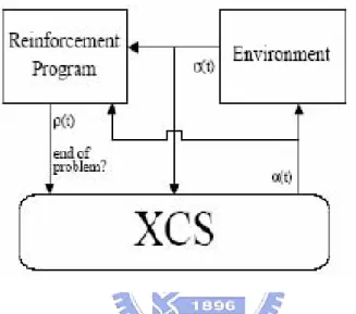
(27) “knowledge” to be readily seen [48] . Financial markets are dynamic environments. Under such circumstances, learning classifier systems can provide the suitable solutions to questions. Learning classifier system technology has been applied in many areas in recent years. For instance, in robotics and automatic driving systems [49], learning classifier systems have been used to develop learning robots. In the area of physician database knowledge access, Holmes [6] proposed the EpiCS platform with the goal of correctly assessing disease risk.. Figure 2-2. Operation diagram of extended classifier systems (Butz & Wilson, 2002) Extended classifier systems (XCS; see Figure 2-2) have the following basic operating procedures: Step 0: Initialization of the classifier population. Step 1: The detector obtains binary environmental state values consisting of (0,1) values from the environment. Step 2: Information is obtained from the detector and used in comparison with the classifier population. If there are no classifiers meeting appropriate conditions in the classifier population, a rule discovery mechanism is used to establish and screen classifiers meeting conditions to a match set. Classifiers meeting the appropriate conditions must incorporate the information obtained by the detector.. 18.

(28) Step 3: Classifiers in the match set are classified according to their action. The predictive value and fitness value of classifiers with identical actions are weighted, yield a prediction array containing prediction values in various states of action. Step 4: Select the prediction values in various states in the prediction array that have the greatest predictive value, and replicate them in the action set. Step 5: The effector is converted according to the action set to another state that can be recognized by the external environment, and performs actions and operations on the external environment. Step 6: The compensation allocation mechanism updates the parameters of all classifiers in the action set with the actual rewards obtained when the effector acted on the environment; actual rewards are used to update the original prediction values, prediction error values, and fitness value parameters. Step 7: A GA operation caused the classifier population to evolve is performed once every fixed interval. After evaluating each classifier's accuracy and experience, inappropriate classifiers are discarded.. Following continuous improvement by many researchers, Wilson proposed an extended classifier system (XCS) in 1995 [63]. Wilson's XCS model strives to achieve accuracy in forecasting returns, eliminates message list, adds prediction arrays and action sets in order to improve classifier system effectiveness, and uses niche-genetic algorithms to implement evolution of rules. Beltrametti, et al. [45] used an LCS model to study the foreign exchange market, the empirical results of this research showed that classifier systems can classify external information and generate suitable predictions, while evolving appropriate trading rules in response to environmental changes. Furthermore, other scholars have used classifier systems to analyze the trading of individual stocks by using price indicators as inputs and 19.

(29) individual stocks sell signals as outputs. For instance, Liao and Chen [76] used price and volume indicators including closing prices, 6-day average prices, and the OBV indicator as input factors, while Schulenburg and Ross [60] used average price and volume as input factors; both obtained experimental results significantly are better than both buy-and-hold and random trading strategies. Multi-agent extended classifier systems use multiple extended classifier systems operating in coordination to achieve even better results from decision-making assistance. Homogeneous or heterogeneous extended classifier systems can individually sense the state of the environment, and the integration of the learning results different extended classifier systems sensing the environment can yield sound recommendations. For instance, a multi-agent extended classifier systems applied to urban traffic congestion providing route recommendations in accordance with news, the weather forecast, and levels of road congestion [46] yield an excellent result. Furthermore, multi-agent extended classifier systems have been applied to air transportation and financial applications. For example, airlines use a heterogeneous multi-agent extended classifier system to solve aircraft route problems [77], and a multi-agent extended classifier system has been used to perform securities research involving many different types of investment targets [71].. 2.4 Technical Analysis Technical analysis is a method of stock price trend analysis that uses statistics or other quantitative methods to convert data consisting chiefly of historical prices and trading volume to charts or indicators with different implications and forecast future stock price trend according to cyclic tendencies to achieve excess returns. Technical analysis is using the “buy-sell” holder historical information to figure out long-short term reflection under the stock market and psychology [16]. After converting historical price and volume data to various indicators, technical analysis can forecast the direction of stock price fluctuations and 20.

(30) trading times. Although many market factors can disturb price trends, technical analysis can still improve the quality of investor decisions. Blume, et al. [44] incorporated trading volume to examine the relationship between price and volume. Their results verified that the signal transmitted by trading volume can reveal price fluctuation information, which implies that the use of trading volume as an auxiliary signal can significantly increase performance. Technical analysis is not a way to accurate the stock price, but it really helps the success probability [5]. Such as CRISMA system [61] used Cumulative Volume, Relative Strength Index, Moving Average to do “ buy and sell decision” With transaction cost or not, CRISMA outperformed the Buy & Hold strategy. Gencay and Stengos adopted Price and Volume Moving Averages, investigated Dow Jones index, explored that Volume can improve predicting ability [56]. Mark used 9K, 9KD, 18ADX, 18MACD, and S&P500 etc. as neural network input factors, this model also predict well [52]. Our study reference those above mentioned input factors, using moving average (MA), stochastic indicators (KD), moving average convergence divergence (MACD), relative strength index (RSI) and Williams %R (WMS %R) as this research model input factors. Kendall and Su [72] used particle swarm optimization to find the best proportion of risk assets. This method, which was based on the mean-variance model and used the Sharpe ratio as its fitness function; although the performance was slightly different, the Kendall and Su method dramatically shortened solution time. Huang and et al.[42] proposed an optimal portfolio capital allocation model, input factor including RSI, BIAS, Psychological Line, Volume Ratio, which employed recurrent neural network to generate decision information and the result discovered about 90% related with the rules extracted by Full-RE algorithm.. 2.5 Summary This study attempts to use evolutionary algorithms to perform research and constructs portfolio insurance decision support models prevent investors from over- or under-reaction, 21.

(31) and reduce common investment mistakes and achieving investment goals. In first stage, we construct decision support model using GAs with stock market raw data as input factors, and using extended classifier systems in second stage with technical indicators as input factors to improve performance of decision support models. Both decision support models are based on TIPP which protects principal and locks in profits is more conservative strategy than other strategies.. 22.

(32) Chapter 3 Design of Decision Support Models This chapter discusses the approach taken by this research. First, it’s an overview of the research framework and the following two sections explain the design of decision support models based on genetic algorithms and extended classifier systems respectively.. 3.1 Research Framework. Figure 3-1.. Research architecture. Conventional economics and financial management research models assume that investors are rational, and consistently take maximization of their own gain as their foremost consideration. Nevertheless, scholars of behavioral finance have recently discovered that people frequently make erroneous decisions due to the isolation effect, framing effect, and so on. In view of the fact that bounded rationality [34] factors often cause people to have decision-making biases, this study has therefore sought to construct a dynamic portfolio insurance decision support model as shown in Figure 3-1. This model is proposed to prevent people from making poor decisions due to the influence of their cognitive biases. 23.

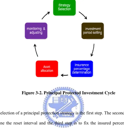
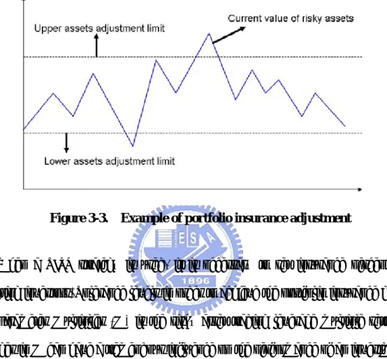
(33) Most principal protected investment employs the five basic operating steps [2] as shown in Figure 3-2.. Figure 3-2. Principal Protected Investment Cycle. Selection of a principal protection strategy is the first step. The second step is to determine the reset interval and the third step is to fix the insured percentage. The fourth step is to allocate the assets which apart from selection financial commodities constituting risky and non-risky assets. The final step is constantly monitoring the state of investment portfolio and adjusting the proportion of risky and non-risky assets. We notice that the above steps as principal protected investment cycle. When the investment period comes to term or adjustment is invalid, we restart a new cycle again. The portfolio insurance adjustment example is shown in Figure 3-3. It reveals that when the current value of assets in an investment portfolio exceeds the upper assets adjustment limit, profit taking will be performed and the assets in the investment portfolio will be adjusted. When the current value of assets in an investment portfolio exceeds the lower assets adjustment limit, assets will be sold at a 24.

(34) loss and the asset allocation in the investment portfolio adjusted. A series of appropriately-timed asset adjustments thus serves to achieve the goal of TIPP strategy.. Figure 3-3.. Example of portfolio insurance adjustment. When a TIPP strategy is used, it is necessary to set insurance percentage reflecting investors' Tolerance levels in order to achieve the portfolio insurance goal. The parameter Multiplier (M) is the risky asset trading leverage multiple setting. Changes in M can have a tremendous influence on the performance of an investment portfolio. It may impossible to protect the principal when M is too large, and market participation will be very low when M is too small [2], which will preclude maximization of returns. Because of this, dynamic adjustment of M which respect to the environment is the only way to achieve the goals of principal protection and maximum returns. Tolerance (T) provides a basis for adjustment exposure to total assets. Trading must be performed to adjust the proportion of risky assets whenever this threshold is exceeded. For instance, if T=5%, trading will be performed when the change in the net value of risky assets exceeds 5%. If, at the time, M=4, no action will be taken when risky assets are in the 3.8-4.2 range. The investment portfolio will be 25.

(35) adjusted again if it exceeds this range. Major factors that affect portfolio insurance performance include trading cost [66]; when trading costs are taken into consideration, the frequency of trades is seen to influence returns on the invested assets. As a consequence, if the T is too small, too many unnecessary trades may be performed during periods of consolidation, and the performance of the portfolio insurance will suffer. Because of this, it is necessary to dynamically select appropriate T values in view of overall market trends in order to avoid needless trading costs. Framing effect is considered a very important psychological bias in the study of behavioral finance. Framing bias notes the tendency of decision maker is respond to various situations differently based on the context in which a choice is presented (framed) [9]. The framing effect refers to when, under circumstances of limited knowledge, investors' reactions to information are invariably reactions directly to the received information, the reality behind which they are unable to scrutinize [53]. Financial investment requires the making of decisions in an uncertain situation. Hence, framing influences decisions. In today's complex financial investment environment, a principal protection investment strategy decision-making assistance model is needed to prevent investors from over- or under-reaction, and help investors to avoid risk and achieve stable return.. 3.2 GA-based TIPP Models Genetic Algorithms (GAs) model genetic evolution. It was first introduced by John Holland [7]. The original GAs are bit string representation, proportional selection and crossover as the primary method to produce new individuals. Up to now, several changes have been developed to the original GAs, which are different representation schemes, selection, crossover, mutation and elitism operators. In this study, each chromosome consists of gene Multiplier and Tolerance. The 26.

(36) relative parameters setting in GA is listed as following. Multiplier：a real number between 0 and 5 Tolerance：a real number between 0 and 10 Population size : 200 Crossover rate : 0.5 Mutation rate : 0.001 Fitness value : Return on Invest(ROI) Termination condition : (1) difference between offspring and parent < 0.000001. or. (2) 1000 generation Training period : 1 year. This research model of TIPP a new portfolio insurance model is based on Continuous Genetic Algorithm (CGA). The objective of proposed model is going to find out an adequate Multiplier, Tolerance for trade and rebalance operating. In this study, we first generate individuals of two times population size, and then select the better 50% of individuals to form the initial population. According to crossover rate, remain the previous generation (1-Pc)*P individuals to the next generation continuously evaluated. The rest individuals are randomly selected from parent individuals, and then mating offspring. The mating process [11] is randomly select nth gene to crossover. For example, consider the two parents to be Parent1 = [Pm1 Pm2 …… PdNpar] Parent2 = [Pd1 Pd2 …… PmNpar] where the m and d subscripts discriminate between the mom and the dad parent. Pm1 represents first gene in mom chromosome, and so forth. Two new genes are generated by following operations. 27.

(37) Pnew1 = Pmn-β（Pmn-Pdn）. (7). Pnew2 = Pdn+β（Pmn-Pdn）. (8). which P represents gene m stands for mom d stands for dad n represents nth gene β is a random value between 0 and 1 and then combine to form new children chromosomes : offspring1 = [Pm1 Pm2 …Pnew1…Pd] offspring2 = [Pd1 Pd2 …Pnew1…Pm]. The next step is mutation operation. Mutation mechanism is avoided evolution converge procedure from the local optimized solution. In this research, we generate a random value, if it is less than mutation rate, mutation operation will be performed. We choose randomly a chromosome and then replace it’s one gene among others by a new value. There are two GA-based models in our research, one is GA optimized TIPP model (GA-TIPP model), another one is GA dynamic optimized TIPP model (GA-DTIPP model). The difference between GA-TIPP and GA-DTIPP models is GA-DTIPP must to find out a new suitable Multiplier and Tolerance after rebalance operation. GA-TIPP keeps two parameters unchanged in investment period. Nevertheless, each Multiplier and Tolerance are generated by GAs after one year training period.. 3.3 XCS-based TIPP Models This model used a TIPP strategy in conjunction with an extended classifier 28.

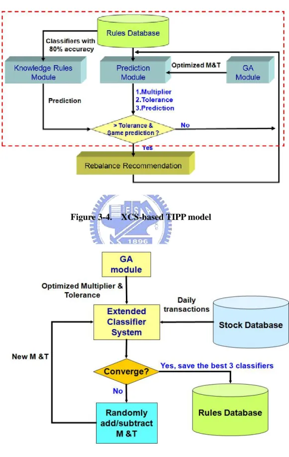
(38) system and genetic algorithms to provide a new portfolio insurance strategy model, investigate the dynamic optimal values of the two variables Multiplier and Tolerance in a changing environment, and to achieve the goal of dynamically adjusting risky asset positions via trend analysis. This module seeks to attain maximum compensation, minimum risk, and minimum trading frequency. This model is as shown in Figure 6. The initial Multiplier and Tolerance values used in this model are optimal values obtained via a GA. The environment rule database is needed by the extended classifier system consists of daily trading data from the Taiwan Stock Exchange input after preprocessing. As shown in Figure 3-4, the extended classifier system model (XCS-based TIPP model) used in this study consists of an environmental rules database and two modules, the prediction extended classifier system module (prediction model) and knowledge rules extended classifier system module (knowledge model). These two modules have different operating mode reflecting their differing goals, and will be described more fully as follows. The XCS-based TIPP model decides whether to make adjustments on the basis of information provided by the prediction module and knowledge model. This study uses the Wilson XCS methodological framework. As for the parameter settings needed in this methodology, settings motivated by differing experimental goals and methods may yield differing results. The parameter settings used in this study are based on the XCS parameter settings employed by Butz and Wilson [48]. Although this study expanded population size to 3,000 in order to accommodate the relatively complex classifier situations in this research.. 29.

(39) Figure 3-4. XCS-based TIPP model. Figure 3-5.. Prediction model 30.

(40) The prediction module performs fine-tuning of M and T via the learning classifier system follow genetic algorithm optimization. Classifier design, data preprocessing, use of genetic algorithms, and the rule database initialization process are explained as follows in accordance with Figure 3-5. The explanation of knowledge model is in Section 3.3.6. 3.3.1 Data Preprocessing Among the technical indicators used in this model, market trading volume and closing index both reveal the state of the environment. The goal of preprocessing is chiefly to convert daily TAIEX trading data to individual technical indicators. The indicators used included 5-day, 22-day, and 60-day MA, 9-day KD, 9-day MACD, and 5-day and 22-day RSI. 3.3.2 Use of Genetic Algorithms Genetic algorithms are employed at two points in this model. One point is outside the XCS-based TIPP model, where a genetic algorithm is used to find optimal Multiplier and Tolerance values as initial inputs in the research model. If Multiplier and Tolerance values are not optimized, it might be necessary to find all possible Multiplier and Tolerance value combinations, or employ random combinations of Multiplier and Tolerance values. These two approaches may result in poor convergence and poor model performance. In this way, this model uses a GA to optimize Multiplier and Tolerance at first, and then it uses these values as the initial inputs in the extended classifier system. The extended classifier system is then subjected to find an adjustment. A genetic algorithm is also used within the extended classifier system. This GA is implicit under the extended classifier system, and chiefly serves as a rule discovery 31.

(41) mechanism and means of optimizing the classifier population. The goal of the external genetic algorithm is to generate the optimal multiple and Tolerance values as initial input values. Evolution to a state of convergence came to a standstill when the population size set at 500. The standard for convergence is under the value generated by one generation which is less than 1/100,000th of that generated by the previous generation. Chromosomes were composed of the two genes Multiplier and Tolerance. The crossover rate was 0.5 the mutation rate was 0.005, and the fitness value was the Sharpe ratio. In accordance with the crossover rate, parent chromosomes meeting conditions (i.e. chromosomes with relatively high fitness value) were retained and paired randomly. The crossover process employed a two-point operation: The locations of two parent genes were switched, yielding two new offspring. The mutation mechanism involved the random change of chromosome and gene locations in accordance with the mutation rate to produce mutation values within the preset range. This study employed a training period of five years. The following is a detailed description of the genetic algorithm process: Steps 0: Multiplier and Tolerance were converted to chromosome gene values. Multiplier: {1.0~10.0}; the corresponding gene values were encoded as {10, 11, 12, 13 ~97, 98, 99, A0} Tolerance: {1.00~10.00}; the corresponding gene values were encoded as {100, 101, 102, ~998, 999, A00} If M was 2.5 and T was 4.68, the encoding would be 25468 Steps 1: Initialization of the population: Randomization was employed to produce 100 first-generation chromosomes. Steps 2: Assessment: The fitness of each chromosome during the training period was assessed by using the Sharpe ratio as a fitness value. The higher the fitness value is, the greater the probability of return during 32.

(42) a cycle. Steps 3: Sorting: Chromosomes were sorted in accordance with chromosome fitness value. Steps 4: Selection: Chromosomes used to produce the next generation were selected accordance with fitness value and the crossover rate. Steps 5: Replication: Members of the chromosome population were paired randomly to produce the next generation. Crossover and mutation were then performed as follows: Crossover: Two random numerical values were generated and used to determine the loci of the genes to be exchanged when parent chromosomes were paired, yielding a new generation of offspring chromosomes. For instance, if the father chromosome was 15482 and the mother 27392, and the random numbers were 1 and 3, then the genes at locations 1 and 3 on the parent chromosomes were exchanged, yielding offspring chromosomes with the values of 25382 and 17492. Mutation: Mutation was implemented in accordance with the mutation rate. The method used was the same by the crossover mechanism. Chromosomes to undergo mutation were randomly selected. One random number determined the location of the gene to mutate, and the second random number was the mutated value. For instance, if the first random number was 2, then the mutation occurred at the second gene, such as the 5 position of the chromosome 15482. The mutated value was also derived from a random number; if the random number was 9, then the mutated chromosome would be 19482. 33.

(43) Regarding the implicit Genetic algorithms, it chiefly serves as a rule discovery mechanism and means of optimizing the classifier population in learning classifier systems. When the model uses a detector to determine the state of the environment, if no classifiers are conforming to that state, it can be found within the classifier population, and then the rule discovery mechanism will be triggered. At that time, the genetic algorithms generate new rules in accordance with the state of the environment to use by the classifier system. With regard to optimization of the classifier population, when the total number of classifiers exceeds the present threshold value or the system model's present implementation interval is over, the genetic algorithm steps of crossover, reproduction, and mutation are employed to cause the classifiers to evolve. Classifiers that are least fit in terms of accuracy and experience are discarded, achieving optimization of the classifier population and improving the system's efficiency. Relevant genetic algorithm design and parameter settings are entirely as defined by Butz and Wilson [48].. 3.3.3 Design of Classifier Condition Portion Each classifier (or rule) is composed of two parts--a condition and an action. As shown in Table 3-1, a classifier's condition portion represents the current state of the environment, and its action portion represents the classifier systems recommendation. In this study, classifier conditions consisted of price indicators (closing price, 5-day MA, 22-day MA, 60-day MA, 9-day KD, 9-day MACD, 5-day RSI, and 22-day RSI) and volume indicators (trading volume). These conditions were converted to binary strings. Classifier action consisted of prediction of the rise or fall of the Taiwan Weighted Stock Index on the next day, with a value of 1 indicating rise and 0 indicating fall.. 34.

(44) Table 3-1. Classifier composition Condition. Action. Condition is composed of technical indicators, closing prices, and trading volume. Prediction of the rise or fall of the Taiwan Weighted Stock Index on the next day. Table 3-2. Classifier condition portions Bit location First bit Second bit Third bit Fourth bit Fifth bit Sixth bit Seventh bit. Eighth and ninth bits. Condition. Value. If xC(t)> x5MA(t). 1. If xC(t)<= x5MA(t) If xC(t)> x22MA(t). 0 1. If xC(t)<= x22MA(t) If x5MA (t)> x22MA(t). 0 1. If x5MA (t)<= x22MA(t) If x5MA (t)> x60MA(t). 0 1. If x5MA (t)<= x60MA(t) If x9K (t)> x9D(t). 0 1. If x9K (t)<= x9D(t). 0. If x5RSI (t)> x22RSI(t). 1. If x5RSI (t)<= x22RSI(t) If xDIF (t)> x9MACD(t). 0 1. If xDIF (t)<= x9MACD(t). 0. If xC(t)> xC(t-1) and v(t)>v(t-1). 11. If xC(t)<= xC(t-1) and v(t)<=v(t-1). 10. If xC(t)> xC(t-1) and v(t)<=v(t-1). 01. If xC(t)<= xC(t-1) and v(t)>v(t-1). 00. 35.

(45) Classifier conditions in the rule database are converted as shown in Table 3-2. The condition portion is composed of nine bits, of which t indicates the date, v(t) indicates trading volume on day t, xC(t) indicates the closing price on day t, and x5MA(t), x22MA(t), and x60MA(t) respectively indicate the 5-day, 22-day, 60-day moving averages on day t, x5RSI(t) and x22RSI(t) respectively indicate the five-day and 22-day RSI on day t, and the remaining items are self-explanatory. With regard to the conversion method, taking the first bit as an example, when xC(t)> x5MA(t), the first bit is set as 1 to express a buy signal; otherwise the first bit is 0. The remaining bits are dealt with in a similar fashion. Table 2 lists the judgment conditions determining bit values. Supposing a certain classifier has a condition portion of 111111111, this conveys the meaning of xC(t)> x5MA(t), xC(t)> x22MA(t), x5MA (t)> x22MA(t), x5MA (t)> x60MA(t), x9K(t)> x9D(t), x5RSI (t)> x22RSI(t), xDIF (t)> x9MACD(t), xC(t)> xC(t-1), and v(t)>v(t-1), all of which are buy signals. The classifier conditions of the Prediction-XCS module and KR-XCS module used in this study employ this design method.. 3.3.4 Design of Classifier Action Portion The chief goal of this model is to predict the rise or fall of the Taiwan Weighted Stock Index on the next day and generate Multiplier and Tolerance values adapted to the current state of the environment. As a consequence, the five-bit action portion of each classifier consists of a stock market rise/fall prediction plus M and T values (see Table 3-3). The first bit of the action portion indicates market rise when it is 1 and fall when it is 0; the second and third bits indicate the M value, and the fourth and fifth bits indicate the T value. For instance, the action portion is 15235 when the market is predicted to rise, the M value is 5.2, and the T value is 3.5%.. 36.

(46) Table 3-3. Composition of classifier action portions First bit Prediction of rise/fall (0/1). Second bit First digit of M value. Third bit Decimal digit of M value. Fourth bit First digit of T value. Fifth bit Decimal digit of T value. 3.3.5 Initialization of The Rule Database The primary goal of this process is to generate an initial population in the rule database. The population size was set as 3,000, and the condition portion consisted of various indicators derived from the actual state of the environment via preprocessing and converted into classifier conditions in accordance with Table 2. The M and T values comprising the action portion were made to evolve via a genetic algorithm to generate optimal input values. In order to investigate possible optimal solutions under different environmental conditions, the model gives the M and T values random weights (0.1, 1.0) during each round of training, until the convergence occurs. The three best classifiers selected on the basis of accuracy (number of profitable trades/total number of trades) are saved in the rule database. When it is more than one classifier has the same accuracy, then returns are used as the basis for selection. If the returns are the same, then roulette wheel method is used to select one classifier. The end of training yields the initial population of the rule database; this population is used during the subsequent testing period.. 3.3.6 Knowledge Rules Model The knowledge model (see Figure 6) is responsible for replicating classifiers with accuracy which greater than 80% that means using this rule(classifier) trading to make profits ten out of eight. We store those rules in the rule database of knowledge rules model. This model is also in charge of backup storage of classifiers representing as the known knowledge rules [17]. Because each classifier is adapted to a certain 37.

(47) environmental state, classifiers with a high accuracy may be discarded due to low triggering probability when the environmental state changes. This model is therefore responsible for uncovering and storing sound knowledge rules for auxiliary decision-making use. With regard to the design of the classifiers in this model, the condition is composed of converted technical indicators as described above, but the action portion constitutes only the prediction of the rise or fall of Taiwan Weighted Stock Index on the next day.. 38.