國 立 交 通 大 學
光 電 工 程 研 究 所
碩士論文
利用 RF 頻譜量測搭配波長掃描調變光源來量測
群速度色散之研究
Novel group velocity dispersion measurement method
by RF spectral analyzer with modulated
wavelength-swept light source
研究生:何姿媛
指導教授:賴暎杰博士
利用 RF 頻譜量測搭配波長掃描調變光源來量測群速
度色散之研究
Novel group velocity dispersion measurement method
by RF spectral analyzer with modulated
wavelength-swept light source
研究生:何姿媛 Student : Zih-Yuan Ho 指導教授:賴暎杰 老師 Advisor : Yin-Chieh Lai
國立交通大學 光電工程研究所
碩士論文
A Thesis
Submitted to Institute of Electro-Optical Engineering College of Electrical Engineering and Computer Science
National Chiao-Tung University
In Partial Fulfillment of the Requirements for the Degree of Master in Electro-Optical Engineering
November 2011
I
摘要
論文名稱:利用 RF 頻譜量測搭配波長掃描調變光源來量測群速度色 散之研究 校所別:國立交通大學光電工程研究所 頁數:1 頁 畢業時間:一百學年度第一學期 學位:碩士 研究生:何姿媛 指導教授:賴暎杰教授 在此光纖通訊日益普遍和被廣泛應用的時代,如何在長距離的光 纖傳輸中保持訊號不失真是一個重要的課題。因為傳輸光纖本身的群 速度色散能影響頻寬和可傳輸的距離,所以群速度色散的經濟有效量 測方法一直也是研究開發上的重點。本論文針對此需求提出一個非干 涉式光纖群速度色散量測方法,僅需 RF 頻譜分析儀而不需更昂貴之 網路分析儀。我們首先利用振幅調變器被加載弦波訊號來調變寬頻光 源的輸出光並透過可調光濾波器來進而得到一個波長掃描式的調變 光源,此光源具有 10GHz 高調變頻率,其中心波長呈慢速的周期性變 化。然後藉由 RF 頻譜分析儀觀察此光源的輸出光經過待測光纖前後 的 RF 頻譜差異,透過進一步地理論分析可以成功得出待測光纖之群 速度色散值,所得結果與已知的光纖規格有很好的吻合。II
ABSTRACT
Title:Novel group velocity dispersion measurement method by RF spectral analyzer with modulated wavelength-swept light source
Pages:1 Page
School:National Chiao Tung University
Department: Institute of Electro-optical Engineering
Time:November, 2011 Degree:Master
Researcher:Zih-Yuan Ho Advisor:Prof. Yin-Chieh Lai Fiber communication has played a major role in the information age nowadays due to the vast advantages of optical fibers over existing copper wires. Since the transmission distance or bandwidth is impacted by the fiber dispersion, the measurement of fiber dispersion has been an important R&D focus. In the thesis, an economic non-interferometric method is developed to measure the group velocity dispersion of optical fibers. A modulated wavelength-swept light source is created with a broadband source followed by an EO modulator and a tunable optical filter. The source is intensity-modulated at the 10GHz high frequency with a slow periodic central wavelength variation. By measuring the RF spectra before and after the light propagates through the test fiber, the group velocity dispersion coefficient of the test fiber can be experimentally determined through the developed theory.
III
ACKNOWLEDGEMENT
關於本篇論文的完成,首先很感謝賴暎杰老師在實驗上鉅細靡遺 地指導,不斷地引導和給意見。使我在專業知識上有很多的進步與提 升,在碩士班兩年的實驗室生涯中,也從老師身上學習到許多研究相 關的經驗。 很感謝陳智弘、鄒志偉老師出借本研究須要用到相關儀器設備, 讓實驗可以順利進行。也很感謝黃淑惠小姐在生活上的照顧及建議, 讓我可以安心地在學校當中完成我的學業。另外,研究中也受到鞠曉 山學長、許怡蘘學姐、徐桂珠學姐、郭立強學長、甘立行學長、王聖 閔學長、吳尚穎學長的指教及關心,還有學弟良愉、國豪、耀德、和 仕斌的支持與幫助。此外,也感謝陳智弘老師實驗室的學長們在本研 究進行中給的資源和熱情的支持,謝謝所有對本研究表達關注與建議 的所有同學及師長們。 最後,特別感謝我的父母和哥哥姊姊對我付出地一切,以及在生 活中包容接納我的教會的姊妹們,希望這份努力的成果可以與你們一 同分享。IV
Contents
Chinese Abstract……….I
English Abstract………....II
Acknowledgement………III
Contents………...……….…IV
List of Figures………..………VI
List of Tables……….….VII
Chapter 1 Introduction
1.1 Overview………...……….………1
1.2 Motivation………...……….………..5
1.3 Thesis organization………...……….………5
References………...…7
Chapter 2 Principles of the GVD Measurement
2.1 ASE broadband light source………..9
2.2 Intensity modulation………10
2.3 The wavelength scanning of a Fabry-Perot tunable filter…14
2.4 Sinusoidal swept-wavelength light source………...18
V
Reference……….…25
Chapter 3 Experimental setup and results
3.1 Experimental setup of the measurement system……..……26
3.2 Analyses with different lengths of fibers…………..……...30
3.2.1 Calculation with first order peak………37
3.2.2 Calculation with second order peak………39
3.3 Discussions………...………...43
3.3.1 The measurement sensitivity………..………43
3.3.2 The measurement limitation………...……45
R
eference……….…47
Chapter 4 Conclusions and Future work
4.1 Summary………..48
VI
LIST OF FIGURES
Fig. 2-1 Generation of amplified spontaneous emission in EDF……….10
Fig. 2-2 An integrated-optical intensity modulator………..13
Fig. 2-3 The transmittance of the Fabry-Perot interferometer varies periodically with the applied voltage V………...14
Fig. 2-4 Fabry-Perot scan to determine the differences in wavelength of two closely spaced wavelength components of the input field………...………16
Fig. 2-5 The fiber-type Fabry-Perot tunable filter………18
Fig. 2-6 The sinusoidal timing position variation……….20
Fig. 2-7 The RF Spectrum of the wavelength-swept light source………22
Fig. 2-8 The scanning range of wavelength induced by applied signal...24
Fig. 3-1 Experiment setup of the dispersion measurement system……..26
Fig. 3-2 The sensitivity of the Fabry-Perot filter………28
Fig. 3-3 The GVD identification process……….30
Fig. 3-4 The optical spectrum around central wavelength 1550nm…….31
Fig. 3-5 The RF spectrum around 10 GHz peak………...32
Fig. 3-6 The RF spectrum with 20m SMF-28 fiber….……….32
Fig. 3-7 The RF spectrum with 100m SMF-28 fiber………33
Fig. 3-8 The RF spectrum with 200m SMF-28 fiber………33
Fig. 3-9 The RF spectrum with 300m SMF-28 fiber………34
Fig. 3-10 The RF spectrum with 500m SMF-28 fiber…..………34
VII
Fig. 3-12 The RF spectrum with 2 km SMF-28 fiber………...35 Fig. 3-13 The RF spectrum with 5 km SMF-28 fiber………...36 Fig. 3-14 The RF spectrum with 10 km SMF-28 fiber……….36 Fig. 3-15 The relation between the length of single mode fiber and the solution of Bessel function………...37 Fig. 3-16 The relation between long fibers and corresponding timing jitter………...38 Fig. 3-17 The relation between short fibers and corresponding timing jitter………...39 Fig. 3-18 The relation between the length of single mode fiber and the solution of Bessel function………...40 Fig. 3-19 The relation between long fibers and corresponding timing jitter………...41 Fig. 3-20 The relation between short fibers and corresponding timing jitter………...41 Fig. 3-21 The peak differences related to fiber length………..44 Fig. 3-22 The peak differences of short SMFs……….45 Fig. 3-23 System original timing variation related to wavelength-swept range……….46
LIST OF TABLES
Table 1-1 Comparison of measurement methods………...4 Table 3-1 The optical devices and instruments ………....29 Table 3-2 The group velocity dispersion coefficient computation……...42
1
Chapter 1
Introduction
1.1 Overview
Group velocity dispersion (GVD) causes a short pulse to spread in time as a result of the fact that different frequency components travel with different group velocities. Large chromatic dispersion may limit the transmission distance and cause the detection errors at the receiver. It is thus important to monitor and control the fiber group velocity dispersion for optical communication applications. In the literature, many GVD measurement methods have been developed and improved continually [1.1]. These include the time-of-flight (TOF) techniques, modulation phase-shift (MPS) methods, temporal/spectral interferometric techniques, and optical time/frequency-domain reflectometric techniques.
The conventional dispersion measurement techniques are categorized and described below. The time-of-flight technique can be used to determine the chromatic dispersion coefficient either by measuring the relative temporal delay between pulses at different wavelengths or by measuring the pulse broadening itself. One of the main problems with the TOF technique is that it generally requires several kilometers of fiber to accumulate an appreciable difference in time for different wavelengths [1.2]. The modulation phase-shift method utilizes the continuous-wave optical signal intensity-modulated by a radio-frequency generator. The optical signal is injected into the fiber under test and the phase of its modulation is measured relative to the electrical modulation driver. The
2
RF phase measurement is repeated at intervals across the wavelength range of interest because the phase difference of the intensity modulation between two wavelengths gives the time delay difference after
propagation. By taking the derivative of the time delay with respect to the
wavelength, the dispersion parameter can be determined [1.3]-[1.5].
Some other precise chromatic dispersion measurement methods are the interferometric methods, which can be categorized into temporal interferometric and spectral interferometric types. Interference fringes in temporal interferometry are produced by two laser beams, one transmitting through the fiber and the other through the air. By superposing two beams coming from the same light source, the interference fringes are obtained. The group delay time difference depends on the optical path lengths through which two beams propagate and can be observed from the coherence term. The spectral phase variation can be extracted from the temporal interferogram if a Fourier Transform is applied to it. The spectral phase contains the dispersion information which can be indirectly obtained by taking the second derivative of the spectral phase. From another point of view, a scan of the wavelength domain in spectral interferometry is performed to produce a spectral interferogram. Two transmitted optical signals are combined to form a cross-correlation interferogram. The chromatic dispersion of a sample fiber can be obtained by measuring the wavelength dependent phase obtained from the spectral interferogram. Because there is no moving part in the experimental setup, the spectral interferometry method is invulnerable to external environments. It has been demonstrated that
3
short fibers can be well characterized by both the temporal and spectral interferometric methods [1.6]-[1.9]. The reflectometric methods of GVD measurement can be briefly described below. The optical frequency domain reflectometry (OFDR) has been proposed to measure the GVD coefficient. A frequency-chirped light source is used and the GVD value is computed directly from the variance of the frequency-chirp rate of the light after propagation through the optical fiber. Owing to two frequency-chirped light sources with a delay time, information of the frequency-chirp rate can be obtained from the beat signal between the light sources. The optical beat signals before transmission in the fiber and after the round-trip transmission are measured. Long-distance measurement can be accomplished only at the input end of the fiber under test [1.10]. Finally a versatile method for the characterization of most types of optical fiber is the optical low-coherence reflectometry (OLCR) technique.The OLCR technique can also be applied to modal chromatic dispersion determination in a system comprising a variety of guided modes with vastly different GVD values [1.12]. An OLCR is basically a Michelson interferometer illuminated by a broadband source where the device under test is inserted in one of the two arms, with the sample arm containing the test fiber, and with a translating mirror in the other arm (the reference arm). Scanning the entire length of the fiber yields two major interferograms (also called reflectograms) due to the reflections at the front and rear cleaved facets of the fiber. The output interferogram is broader than the input one owing to the chromatic dispersion of the fiber. The group delay is simply obtained by differentiating the facet
4
reflectivities in the spectral domain [1.11].
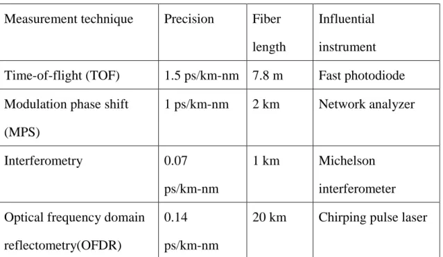
The time-of-flight methods require high peak power pulses and fast pulse detection. Interferometric measurements are not suitable for long fibers for communication uses. In conventional techniques the utilized optical sources have restricted measurable spectral ranges, the continuity of spectral ranges or time resolution. Based on the research in the past, convenient configuration and less measuring time are interesting issues for engineers to reduce cost. The MPS method is a standard non-interferometric technique used in most of the optical fiber manufacturing companies, since the method allows accurate and simple measurement of the fiber chromatic dispersion. However, an expansive network analyzer is needed to determine the RF modulation phase. In this thesis work we want to develop a new non-interferometric method that does not require the expansive network analyzer.
Table 1-1 Comparison of measurement methods
Measurement technique Precision Fiber
length
Influential
instrument
Time-of-flight (TOF) 1.5 ps/km-nm 7.8 m Fast photodiode
Modulation phase shift
(MPS) 1 ps/km-nm 2 km Network analyzer Interferometry 0.07 ps/km-nm 1 km Michelson interferometer
Optical frequency domain
reflectometry(OFDR)
0.14
ps/km-nm
5
1.2 Motivation
In this work we propose a novel group velocity dispersion measurement method with a frequency swept light source. The measurement system consists of an amplified spontaneous emission (ASE) C-band light source which output beam is modulated by a Mach-Zehnder EO modulator driven by a sinusoidally varying electric voltage from a synthesizer. Complex laser pulse sources and numerous optical components are not required in the experiment setup. It also eliminates nonlinear effects that may be resulted from the laser cavity. A fiber-type Fabry-Perot tunable filter plays an important role for this experimental setup. Based on the frequency scanning characteristics of the filter, a periodically wavelength-swept light source is obtained by tuning the piezoelectric control of the filter etalon spacing. By measuring the frequency sub-components of the modulated light on the RF spectrum analyzer before and after connecting the test single mode fiber, the fiber group velocity dispersion can be determined, as to be explained below. We put simple physical concepts to new uses in this method without requiring complex mathematical modeling.
1.3 Thesis organization
This thesis is consisted of four chapters. Chapter 1 is an overview of the group velocity dispersion measurement techniques. Chapter 2 describes the theory of frequency swept mechanism and the mathematical analysis. Chapter 3 explains the experimental setup and results which
6
demonstrate the conditions that this new method can be used. Finally Chapter 4 presents the conclusion and summary which indicate the possible applications. Future work that can be explored is also discussed.
7
References
[1.1] L. G. Cohen, “Comparison of Single-Mode Fiber Dispersion Measurement Techniques,” J. Lightwave Technol. LT-3, 958-966, 1985. [1.2] J. M. Wiesenfeld and J. Stone, “Measurement of Dispersion Using Short Lengths of an Optical Fiber and Picosecond Pulses from Semiconductor Film Lasers,” J. Lightwave Technol. LT-2, 464-468, 1984.
[1.3] M. A. Galle, “Single-arm three wave interferometer for measuring dispersion in short lengths of fiber,” a thesis submitted in conformity with the requirements for the degree of Master of Applied Science at the Graduate Department of Electrical & Computer Engineering, University of Toronto, 2007.
[1.4] L. Cherbi, M. Mehenni, and R. Aksas, ”Experimental Investigation of the Modulation Phase-Shift Method for the Measure of the Chromatic Dispersion in a Single-Mode Fiber Coiled on a Covered Spool,” Microw Opt. Techn. Let. 48, 174-178, 2006.
[1.5] K. Mori, T. Morioka and M. Saruwatari, “Ultra-wide Spectral Range Group Velocity Dispersion Measurement of Single-Mode Fibers Using LD-Pumped Supercontinuum in an Optical Fiber,” IEEE Instrumentation and Measurement Technology Conference 1994, Hamamatsu, Japan, May 10-12, 1994, paper THAM 9-4.
[1.6] M. Tateda, N. Shibata, and S. Seikai, ”Interferometric Method for Chromatic Dispersion Measurement in a Single-Mode Optical Fiber,” IEEE J. Quantum Elect. QE-17, 404-407, 1981.
8
measurement using the Fourier transform of an interferometric cross correlation generated by white light,“ Opt. Lett. 15, 393-395, 1990.
[1.8] P. Böswetter,* T. Baselt, F. Ebert, F. Basan, and P. Hartmann, “Evaluation of a time-frequency domain interferometer for simultaneous group-velocity dispersion measurements in multimode photonic crystal fibers,” Appl. Opics. 50, 32-37, 2011
[1.9] J. Y. Lee and D. Y. Kim, ” Versatile chromatic dispersion measurement of a single mode fiber using spectral white light interferometry,” Opt. Express 14, 11608-11615, 2006.
[1.10] M. Yoshida, T. Miyamoto, K. Nakamura, and H. Ito, “A New Technique for Measuring Dispersion of Optical Fibers Using a Frequency-Shifted Feedback Fiber Laser. Part I: Measurement of Group Velocity Dispersion,” Electron. Comm. Jpn. 1, 85, 1-7, 2002
[1.11] R. Gabet, P. Hamel, Y. Jaouën, A.-F. Obaton, V. Lanticq, and G. Debarge, “Versatile Characterization of Specialty Fibers Using the Phase-Sensitive Optical Low-Coherence Reflectometry Technique,” J. Lightwave Technol. 27, 3021-3033, 2009.
[1.12] P. Hamel, Y. Jaouën, and R. Gabet, ” Optical low-coherence reflectometry for complete chromatic dispersion characterization of few-mode fibers,” Opt. Lett. 32, 1029-1031, 2007.
9
Chapter 2
Principles of the GVD Measurement
2.1 ASE broadband light source
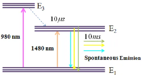
An ASE source usually uses rare earth-doped optical fibers such as Erbium doped fibers (EDFs) to be the optical amplification media. For EDFs, There are two commonly-used pumping-bands, 980nm and 1480 nm, characterized by different absorption cross-sections. The combinational usage of both 980 nm and 1480 nm pumping is also often seen today. The excitation processes of 980 nm and 1480 nm pumping system are both three-energy-level-like. The energy levels of Erbium ions are depicted in Fig. 2-1 and the mechanism of amplified spontaneous emission of 980 nm pumping is explained below [1].
When a laser gain medium is pumped by a laser diode, population inversion is produced with Erbium ions aggregating in the higher energy level E3. The stimulated electrons will rapidly fall into the lower energy
state E2 via non-radiative transition in 10
s . Since the energy states, E1and E2, are affected by internal coupling, the energy states are unevenly
split due to the Stark effect. Finally some photons spontaneously drop to the ground state E1 owing to the 10 ms life time of the energy state E2.
The output spontaneous emission with a broadband range approximately from 1530 nm~1565 nm is generated. The ASE broadband light therefore has random emission phases and directions. The ASE light sources typically feature high output power, wide spectral range and high stability against temperature change.
10
Fig. 2-1 Generation of amplified spontaneous emission in EDF
2.2 Intensity modulation
Optical fiber is the most common type of channel for optical communication and the way of signal encoding is typically simple intensity modulation. Since it may be difficult to directly modulate the amplitude or phase of the semiconductor lasers at a high rate with good signal quality, an external modulator using the electro-optic effect may be necessary [2]. A phase modulating electro-optic modulator (EOM) can also be used as amplitude modulator by incorporating a Mach-Zehnder interferometer setup. A beam splitter divides input light into two paths, and one of the light paths has an EOM driven by external voltage. Since the phase of the light exiting an EOM is controlled by changing the electric field in the EO crystal, changing the electric field on the phase modulating path will then determine whether the two beams interfere constructively or destructively at the output, and thereby control the amplitude or intensity of the exiting light.
11
where the refractive index of an electro-optic medium such as LiNbO3 is
a function of an applied steady electric field E. It can be expanded in a Taylor series about E 0,
...
2
1
)
(
E
n
a
1E
a
2E
2
n
(2. 1)where the coefficients of expressions are
n
n
(
0
)
,a
1
(
dn
dE
)
E0 ,and 0
2 2
2
(
d
n
dE
)
Ea
. We define two electro-optic coefficients3 1 2a n
ands
a
2n
3 , so that.
2
1
2
1
)
(
E
n
n
3E
sn
3E
2
n
(2.2)Terms higher than the third can safely be neglected.
In a Pockels medium, the third term in (2.2) is negligible in comparison to the second. Hence
E n n E n 3 2 1 ) (
(2.3)The coefficient is called the Pockels coefficient or the linear electro-optic coefficient. Clearly it could be shown that the Pockles cell can play the role as a phase modulator. When a beam of light is traveling through the Pockels medium of length L to which an electric field is applied, it undergoes a phase shift
n
(
E
)
k
0L
2
n
(
E
)
L
0, where0
is the free space wavelength. By substituting Eq. (2.3) we have, 0 3 0 n EL (2.4)
12
where
0 2
nL
0. If a voltage V is applied to induce the electric filed E across two faces of the medium separated by d, then E V d . Eq. (2.4) becomes,
0
V
V
(2.5) where.
3 0n
L
d
V
(2.6) The parameterV
, known as the half-wave voltage, is the applied voltage at which the phase shift changes by
. It is obvious that we can modulate the phase of light by changing the applied voltage across the EO material through which the beam of light passes.Electro-optics can be constructed as integrated-optical devices which operate at higher speeds and lower voltages than bulk devices do. The transverse configuration especially lowers the aspect ratio d L and makes the maximum operation speeds in excess of 100 GHz, where light can be easily coupled into, or out of, the modulator by use of standard single mode fibers.
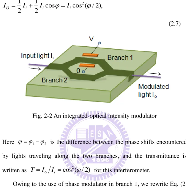
We will then explain how the Mach-Zehnder intensity modulator is formed by simply incorporating the phase modulator described above into one path of the Mach-Zehnder interferometer as in Fig. 2-2. It is known that a beam of light is directed into the Mach-Zehnder interferometer through the fiber pigtail with its power divided equally in each path. The output intensity is given by
13 ), 2 / ( cos cos 2 1 2 1
2
i i i O I I I I (2.7)Fig. 2-2 An integrated-optical intensity modulator
Here 1 2 is the difference between the phase shifts encountered
by lights traveling along the two branches, and the transmittance is written as T IO Ii cos2(
/2) for this interferometer.Owing to the use of phase modulator in branch 1, we rewrite Eq. (2. 5) as
1
10
V V and substitute it into 1 . Finally
1 2 0 V V is obtained, where the constant
0
10
2depends on the optical path difference. Therefore transmittance of the Mach-Zehnder interferometer is a function of applied voltage,
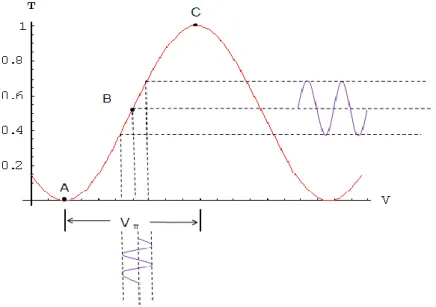
) 2 2 ( cos ) ( 2 0 V V V T , (2.8)
where it is plotted in Fig. 2-3 with an arbitrary 0.
14
linear region of the device. The goal is achieved by adjusting the optical path length to satisfy the initial condition
0
2.Fig. 2-3 The transmittance of the Fabry-Perot interferometer varies periodically with the applied voltage V
The sinusoidal modulation of the MZM produces high order side peaks presenting at two sides of the central carrier frequency. By adjusting the external bias voltage, even or odd sidebands will appear on the RF spectrum analyzer [3]. The modulation frequency is at 10GHz in our case to ensure that distinct side peaks can be observed and higher sensitivity is achieved. Further analysis will be discussed in later sections.
2.3 The wavelength scanning of a Fabry-Perot tunable filter
We will consider the conventional Fabry-Perot interferometer setup to understand how a fiber-type Fabry-Perot tunable filter can provide wavelength selection. For our purpose, it is used to scan wavelengths in a
15
specific range periodically.
The Fabry-Perot interferometer consists of an external source and two parallel plates, which form a cavity. And the mirror separation can be controlled by means of a piezoelectric spacer. The length of air gap between the two surfaces in the Fabry-Perot interferometer decides the round-trip phase shift of the light traveling in the cavity and thus also the transmittance spectrum in the steady-state. For example, the transmittance reaches the maximum for a scanning Fabry-Perot interferometer whenever [4]
.
2
2
2
2
kd
d
m
m 0,1,2... (2.9) Rearrangement gives the condition for a maximum as.
2
m
d
m
(2.10) Accordingly, the free “spatial” range in this mode of operation is.
2
1
m m fsrd
d
d
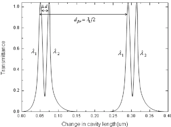
(2.11) Eq. (2.11) is usually used to calibrate the cavity length change in order to determine the difference in wavelength of two closely spaced wavelength components in the input to the Fabry-Perot cavity. An example of a record that would result when light of two different but closely spaced wavelengths
1and 2 are simultaneously input into a16
Fig. 2-4 Fabry-Perot scan to determine the differences in wavelength of two closely spaced wavelength components of the input field
If
1 and 2 are very near to a nominal wavelength
, thisrecord can be used to accurately decide the wavelength difference of the two input wavelengths. If it is known that the adjacent peaks in Fig. 2-4 have the same mode number m, then the wavelengths must satisfy the relations
,
2
1 1
d
m
.
2
2 2
d
m
The wavelength difference is then,
,
)
2
(
2
)
(
2
1 1 1 2 1 2d
d
d
d
m
17 and thus
.
1 1d
d
(2.12) Although the absolute length of the cavity is unlikely to be known toa high degree of accuracy, we can use the nominal length d d1 of the
cavity in this expression. And we typically replace the wavelength
1 inEq. (2.12) by its nominal value
. Eq. (2.12) also demonstrates the limiting level which the Fabry-Perot interferometer can ultimately resolve. In other words, the goal of transmission wavelengths scanning can be achieved by periodically changing the separating distance of Fabry-Perot etalon. Furthermore the mirror separation is tunable by an AC signal from an arbitrary function generator, which will be particularly explained in next section.The piezoelectric effect is the major mechanism to understand the foregoing concepts of Fabry-Perot filter tunability. Piezoelectric effect is the linear electromechanical interaction between the mechanical and the electrical state in some crystalline materials. The piezoelectric crystal experiences mechanical deformation when an external voltage is applied while the internal generation of electrical charge results from an applied mechanical force. Piezoelectric material is installed in a piezo controller and functions as a flexible material in order to fine tune the separating distance between the reflecting surfaces of the filter cavity. We have used a fiber-type Fabry-Perot filter with fundamental characteristics of the original invention to replace the old, bulk-optic Fabry-Perot
18
interferometers. The advanced technical attributes are shown as follows. By adding a segment of optical fiber within the original Fabry-Perot
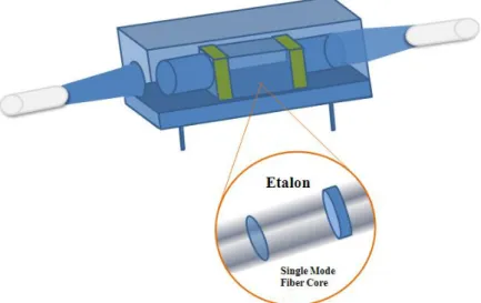
etalon in our case, a fiber-type Fabry-Perot filter can be created and developed as shown in Fig. 2-5. The all-fiber etalon contains no lenses or collimating optics, and thus has superior beam guiding technique by avoiding vibration sensitivities. When an electric field is applied to the fiber Fabry-Perot filter, the cavity length in etalon will change so that the transmission wavelength difference is induced according to Eq. (2.12).
Fig. 2-5 The fiber-type Fabry-Perot tunable filter
2.4 Sinusoidal swept-wavelength light source
Different frequency components traveling in the dispersion media such as optical fibers experience distinct velocities and we will choose a suitable light source in order to demonstrate obvious physical quantity of variation on the radio-frequency spectrum analyzer. In this case, a fast sinusoidal intensity-modulated signal with slow periodical wavelength
19
variation is generated from a broadband light source. The optical intensity is transformed into photocurrent by the fast photodiode and becomes the electrical power on the RF analyzer. The optical intensity going through the fiber under test (FUM) can be expressed by
] )) ( ( cos[ 2 1 2 1 ) ) sin( cos( 2 1 2 1 cos 2 1 2 1 0 0 t s t I I t s t I I I I I p i i f p p i i i i O (2.13) where Eq. (2.7) is utilized and simplified based on some assumptions. Here
p is the angular frequency of Mach-Zehnder modulator outputlight,
s
is the half peak-to-peak displacement of the slow sinusoidal timing variation,s
(
t
)
s
sin(
ft
)
, which is induced by the centerwavelength scan after passing through a section of test optical fiber connected after this light source. Finally,
f stands for the angularfrequency of the slow modulating sinusoidal signal. The device may be operated as a linear intensity modulator when the Mach-Zehnder modulator works in the linear region in Fig. 2-3 with the external modulating sinusoidal function V biased at the point B from signal generator. The slow periodical center wavelength scan of the narrowband output light is created via a Fabry-Perot tunable filter. The photocurrent from the fast photodiode can therefore be written by:
20
,
)
(
)
exp(
)
exp(
4
1
)
(
)
exp(
)
exp(
4
1
2
1
]
))
(
(
cos[
2
1
2
1
)
(
2 0 2 0 0
n in t in p n n p i n in t in p n n p i i p i i oe
e
s
J
i
t
j
j
I
e
e
s
J
i
t
j
j
I
I
t
s
t
I
I
t
I
f f
(2.14)where
J
n(
)
represents the Bessel function of first kind of order n [5].The periodic sinusoidal modulation effects can be illustrated as shown in Fig. 2-6.
21
Other variables like temperature, humidity and pulse energy variation can be safely eliminated due to the fact that only the intensity ratio is utilized and the experiment can be finished in short time. The assumption is reasonable due to the variation of those variables only contributing very small percentage in total.
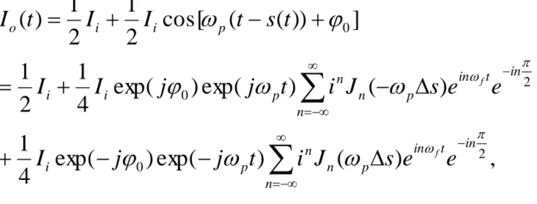
The signal is observed on the RF spectrum analyzer after Fourier transform and can be written as
,
)
(
)
(
)
(
)
exp(
4
1
)
(
)
(
)
(
)
exp(
4
1
)
(
2
1
)
(
2 0 2 0
n f in p n n p i n f in p n n p i in
e
s
J
i
j
I
n
e
s
J
i
j
I
I
I
(2.15) where () is the Dirac delta function. The first term can be regarded as a DC bias signal, and the third major term of negative frequency components can be ignored since it is just the conjugate of the positive frequency term. We can merely consider the second term and it is a Dirac delta distribution over the whole frequency domain. The function characterizes a central frequency
p with evenly expanded sub-components of interval
f caused by slow periodic sinusoidalmodulation. The side peaks have unique power ratios proportional to the square of Bessel functions as shown in Fig. 2-7. The half peak-to-peak displacement of the slow sinusoidal timing variation
s
is determined by the intensity ratio between the zero-th order and first order from the22 experimental data,
. 2 1 0 2 1 0 s J s J s J s J p p p p (2.16)Fig. 2-7 The RF Spectrum of the wavelength-swept light source
2.5 Sinusoidal variation of the center wavelength
The deformation of cavity length d in the Fabry-Perot filter is driven by the sinusoidal voltage signal of the signal generator, and the periodic variation of separating distance d leads to sinusoidal wavelength scanning
of the light which passes through the Fabry-Perot filter.
contributes to the signal timing variation through the dispersion effect of the test optical fiber and we can rewrite s(t) in Eq. (2.13) as)
sin(
)
(
t
DL
t
23
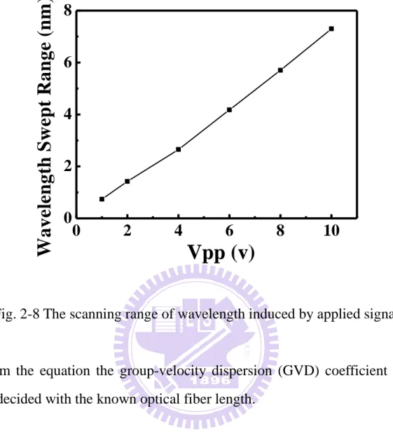
coefficient of test fibers, and L is the length of fibers used. In order to achieve higher resolution of the observation, it is essential to increase the range for wavelength scanning. It is thus important for this experiment to calibrate the wavelength change when an external voltage signal is applied.
The fitting line in Fig. 2-8 shows how the tuning range of wavelength depends on the applied voltage, and the scattering experimental data points of
exhibit a high degree of linear relation. It reveals that the larger the AC signal becomes, the wider the scanning wavelength range gets. To improve the resolution for the experiment, we choose the max applied voltage to ensure the widest scanning range. According to the discussion above, the peak power intensity ratio in Eq. (2.16) can be rewritten as
. 2 1 0 2 1 0 DL J DL J DL J DL J p p p p (2.17) We assume that the peak power of the zero-th and the first order are respectively IA and IB, and the differences between them are equal to
DL
J DL J s J s J I I p p p p B A 1 0 10 1 0 10 10 log 20 log 20 log 10 (2.18)24
0
2
4
6
8
10
0
2
4
6
8
W
a
v
e
le
n
g
th
S
w
e
p
t
R
a
n
g
e
(
n
m
)
Vpp (v)
Fig. 2-8 The scanning range of wavelength induced by applied signal
From the equation the group-velocity dispersion (GVD) coefficient can be decided with the known optical fiber length.
25
References
[1] 陳威廷,“寬頻摻鉺光纖放大器之優化研製”,台灣科技大學碩 士論文 , 2007.
[2] B. E. A. Saleh, and M. C. Teich, “Fundamentals of photonics,” second edition, John Wiley &Sons, New Jersey, 2007.
[3] C. T. Lin, P. T. Shih, J. H. Chen, W. J. Jiang, S. P. Dai, P. C. Peng, Y. L. Ho, and S. Chi, “Optical Millimeter-Wave Up-Conversion Employing Frequency Quadrupling Without Optical Filtering,” IEEE T. MICROW. THEORY. 57, 2084-2092, 2009
[4] F. L. Pedrotti, L. M. Pedrotti, and L. S. Pedrotti, “Introduction to Optics, “third edition, Person Prentice Hall, New Jersey, 2006
[5] E. Kreyszig, “Advanced Engineering Mathematics, “eighth edition, John Wiley &Sons, New York, 1999
26
Chapter 3
Experimental setup and results
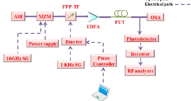
3.1 Experimental setup of the measurement system
The detailed statement of group-velocity dispersion measurement principles has been adequately discussed in previous sections. We will explore the working mechanism and achievements of the measurement system further in this section. The schematic setup of our novel dispersion measurement system is shown in Fig. 3-1, which can be divided into two parts. Firstly, the wavelength swept light source has the slow periodic wavelength variation of intensity-modulated light and the light goes through the fiber under test which will induce timing variation of the signal through the dispersion effects. Secondly, the optical signal is detected by a fast photodiode followed by a RF spectrum analyzer so that the group-velocity dispersion coefficient of the test optical fiber can be obtained by directly analyzing the frequency spectrum.
27
The wavelength-swept light source utilizes slow sinusoidal wavelength filtering to an originally broadband signal with fast intensity modulation. A Mach-Zehnder modulator provides the white light beam with amplitude modulation and operates at a speed around 10 GHz in order to enhance the detection sensitivity. The external modulation method is relatively expensive but reduces chirp quite substantially. It is constructed as transverse integrated-optical devices with lower operating voltages. The light can be conveniently coupled into, and out of, the modulator by the use of optical fibers. The waveguide is fabricated in an electro-optical substrate (often LiNbO3) by diffusing materials such as
titanium to increase the refractive index. When the electro-optic modulator is biased by a DC power supply at half-wave voltage, we ensure that this device works in the linear region. A bias tee is a three port network used for setting the DC bias point of some electronic components without disturbing other components. The low frequency port is used to set the bias by the a piezo controller; the high frequency port passes the radio frequency signals but blocks the biasing levels; the combined output port is connected to the Fabry-Perot filter, which sees both the bias and RF [1]. The sinusoidal signal of 1kHz is therefore applied through the bias-tee device.
An Erbium doped fiber amplifier (EDFA) is put before the fiber under test to function as a power amplifier to provide enough optical power. An amplified spontaneous emission light source typically has high output power, wide spectral range, large spectral bandwidth, and high stability against temperature change.
28
The fiber-type Fabry-Perot tunable filter (FFP-TF) generates wavelength-tunable narrowband signals and its lensless fiber construction allows high finesse and low loss transmission profile. The filter is applied to the light passing through the Mach-Zehnder modulator so as to induce a slow varying sinusoidal wavelength scanning. The piezo controller is driven by the LABVIEW software of the computer to change the etalon length of FFP-TF for periodic wavelength scanning.
The temperature test of the fiber-type Fabry-Perot filter is shown in figure 3-2. When the Fabry-Perot filter is heated by a hot plate, its center wavelength is shifted to the longer wavelength. From the fitting line, we can discover that center wavelength approximately increases 0.57 nm while temperature rises by 1℃.
26
28
30
32
34
36
1550
1552
1554
1556
C
e
n
te
r
W
a
v
e
le
n
g
th
(n
m
)
Temperature (
C)
Data C.W.=1536.094+0.57* temperature29
Table 3-1 The optical devices and instruments
1. ASE light source : maximum output power : 17.17 mW 2. Mach-Zehnder modulator
3. Signal generator 2
4. Fiber Fabry-Perot tunable filter : central wavelength : 1520~1570 nm 5. Bias T
6. Piezo controller : 0~150V
7. Erbium doped fiber amplifier : signal gain : 25dB 8. Photo detector
9. Receiver 10. Hot plate
The broad band light ASE source is indirectly modulated and output a periodically sinusoidal wavelength-swept light beam. The gradual scanning of the selected wavelength bandwidth will induce timing variation owing to the dispersion effect of the added section of single mode fiber. There are two steps in Fig. 3-3 which explain the process for dispersion measurement. First, the output light of the wavelength-swept light source displays spectrogram on the optical spectrum analyzer, and the scanning range of wavelength is variable by adjusting amplitude of the low frequency signal generator. The value of
is then calibrated for certain applied signal and DC bias. Secondly, the light passes through a single mode fiber and produces a frequency spectrum on the RF30
spectrum analyzer. The specific timing jitter
s
is therefore obtained, and the group-velocity dispersion coefficient of the test fiber is inferred with the known
.Fig. 3-3 The GVD identification process
3.2 Analyses with different lengths of fiber
The different lengths of single mode fiber introduce different magnitudes of dispersion effects. By making use of the periodic swept-wavelength light source, the group-velocity dispersion coefficient can be efficiently identified within minutes. The optical spectrum of the light source output is depicted in Fig. 3-4. The optical spectrum exhibits an inverse parabolic shape because the spectral edges have longer integration time than the central part due to the sinusoidal swept operation of the tunable filter. The scan speed of central band is faster than two edges. The largest wavelength scanning band that can be achieved with our current ASE source is selected to enhance the measurement sensitivity for the following measurements. The periodic wavelength-swept range is about 7 nm, and its half peak-to-peak value,
31 1540 1545 1550 1555 -48 -46 -44 -42 -40 -38 -36 -34
In
te
n
si
ty
(d
B
m
)
wavelength(nm)
7 nm
Fig. 3-4 The optical spectrum around central wavelength 1550nm
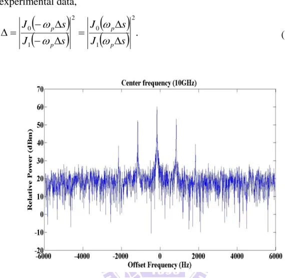
The RF spectrum of the light source output is shown in Fig.3-5. The magnitude of sinusoidal timing variation will be changed when different types of external fibers are added. The frequency of sinusoidal timing variation is 1 kHz, which is set at first. The slow sinusoidal wavelength filtering applied onto the output light of the Mach-Zehnder modulator produces high order peaks around the central peak on the RF spectrum.
Spectra of different lengths of single mode fiber are plotted in Fig. 3-6 to Fig. 3-14. The timing jitters induced by these external fibers are calculated by Eq. (2.18) and from them the experimental value of group velocity dispersion parameter D is obtained. It obviously shows excellent consistency with the known value of standard SMF fibers, 17 ps/km-nm [2].
32 9.996 9.998 10.000 10.002 10.004 -100 -80 -60 -40 -20 Sapn 10kHz RBW 10Hz
In
te
n
si
ty
(
d
B
m
)
RF spectrum (GHz)
1kHz
Fig. 3-5 The RF spectrum around 10 GHz peak
9.996 9.998 10.000 10.002 10.004 -120 -90 -60 -30
In
te
n
si
ty
(
d
B
m
)
Frequency (GHz)
33 9.996 9.998 10.000 10.002 10.004 -120 -90 -60 -30
In
te
n
si
ty
(
d
B
m
)
Frequency (Hz)
Fig. 3-7 The RF spectrum with 100m SMF-28 fiber
9.996 9.998 10.000 10.002 10.004 -120 -90 -60 -30
In
te
n
si
ty
(
d
B
m
)
Frequency (Hz)
34 9.996 9.998 10.000 10.002 10.004 -120 -90 -60 -30
In
te
n
si
ty
(
d
B
m
)
Frequency (Hz)
Fig. 3-9 The RF spectrum with 300m SMF-28 fiber
9.996 9.998 10.000 10.002 10.004 -120 -90 -60 -30
In
te
n
si
ty
(
d
B
m
)
Frequency (GHz)
35 9.996 9.998 10.000 10.002 10.004 -120 -90 -60
In
te
n
si
ty
(
d
B
m
)
Frequency (GHz)
Fig. 3-11 The RF spectrum with 1 km SMF-28 fiber
9.996 9.998 10.000 10.002 10.004 -120 -90 -60
In
te
n
si
ty
(
d
B
m
)
Frequency (GHz)
36 9.996 9.998 10.000 10.002 10.004 -120 -90 -60
In
te
n
si
ty
(
d
B
m
)
Frequency (GHz)
Fig. 3-13 The RF spectrum with 5 km SMF-28 fiber
9.996 9.998 10.000 10.002 10.004 -120 -90 -60
In
te
n
si
ty
(
d
B
m
)
Frequency (GHz)
37
3.2.1 Calculation with first order peak
The Fig. 3-15 adopts the peak power difference of the zero-th order component and first order component in the RF spectra shown in figure 3-5 to 3-14. The almost linear relation between lengths of fibers and the Bessel function solutions demonstrate the consistency of the measured group velocity dispersion coefficient.
0
2
4
6
8
10
0
5
10
15
20
25
30
35
40
B
e
ss
e
l
fu
n
c
ti
o
n
s
o
lu
ti
o
n
(
r
a
d
ia
n
)
Fiber length (km)
Fig. 3-15 The relation between the length of single mode fiber and the solution of Bessel function
Because the slope above has slight discrepancy in the short and long lengths separated by 1km, we divide the measurements into short and long fiber lengths in Fig. 3-16 and Fig. 3-17. The timing jitter is directly obtained from Bessel function solution, and the original data D is very
38
close to the fitting straight line. The experimental value of group velocity dispersion coefficient can be approximately evaluated from slope of the fitting lines in these figures. The GVD value of the long fiber class is 16.95 ps/km-nm, and the GVD value of the short fibers is 16.67 ps/km-nm. When there is no fiber connected, the system still has 0.48 ps timing jitter as detected, which should be due to the detection noises and the fiber dispersion of the light source.
0 2 4 6 8 10 0 100 200 300 400 500 600
s
(p
s)
SMF Length (km)
Data s=-17.8+59.32* SMF length39
0.0
0.1
0.2
0.3
0.4
0.5
0 5 10 15 20 25 30
s
(p
s)
SMF Length (km)
Data s=0.45+58.35*SMF Length 0.48 psFig. 3-17 The relation between short fibers and corresponding timing jitter
3.2.2 Calculation with second order peak
According to the power spectra of different lengths of single mode fiber presented above, the peak power difference of the zero-th order and the second order peak can also be computed to identify the feasibility of this method when higher order peaks are utilized. The linear relation between fiber lengths and the Bessel function solutions demonstrates stability of the experiment system.
40 0 2 4 6 8 10 0 5 10 15 20 25 30 35 40
B
e
ss
e
l
fu
n
c
ti
o
n
s
o
lu
ti
o
n
(
r
a
d
ia
n
)
Fiber length (km)
Fig. 3-18 The relation between the length of single mode fiber and the solution of Bessel function
Based on the above-mentioned reasons, these fibers are again classified in the cases of the second order peak. The timing jitter becomes larger as the fiber length gets longer in figure 3-19 and 3-20. A straight line fits the scattering data points and the believable slope is given. The GVD value of the long fibers is estimated to be 16.75 ps/km-nm, and the GVD value of the short fibers is 16.45 ps/km-nm.
41 0 2 4 6 8 10 0 100 200 300 400 500 600
s
(p
s)
SMF Length (km)
Data s=-18.94+58.64*SMF lengthFig. 3-19 The relation between long fibers and corresponding timing jitter
0.0 0.1 0.2 0.3 0.4 0.5 0 5 10 15 20 25 30
s
(p
s)
SMF Length (km)
Data s=0.83+57.57* SMF length 1.09 psFig. 3-20 The relation between short fibers and corresponding timing jitter
When there is no extra fiber added, little timing jitter is still found. The original timing jitter verifies the experiment limitation of this system,
42
and it may be resulted from the detection noises. It will be discussed in the next section. Besides, a message is revealed from the observation of the timing jitter relation when different lengths of fiber are used. When L is small, the Bessel function values at higher order peaks are much smaller than the lower order. It means that the signals are more degraded by noises at higher order peaks and thus the value of original timing jitter 1.09 ps is bigger than 0.48 ps of the first order peak. The D of the first order peak is thus more close to standard value of single mode fiber than that of the second order peak, which is arranged in table 3-2.
Table 3-2 The group velocity dispersion coefficient computation
Fiber length (km ) D (ps/km-nm) 0.02~0.5 1~10 2 1 0 ) ( ) ( s J s J p P 16.67 16.95 2 2 0 ) ( ) ( s J s J p p 16.45 16.75
The group velocity dispersion coefficient can be evaluated from the theoretical value of slope in the relation between timing jitter and fiber length. From the arrangement in table 3-2, group velocity dispersion coefficients from different lengths and different orders are listed, and all the estimated values are close to the standard D of single mode fiber, 17 ps/nm-km. There is small difference of the D values between short and
43
long fibers since the short fibers are Corning SMF while the long fibers are SMF from POFC. The results demonstrate the precision of the novel dispersion measurement method.
3.3 Analyses
3.3.1 The measurement sensitivity
The difference between zero order peak and other order peaks changes as the fiber length increases from 20 m to 10 km, shown in Fig. 3-21. It shows the sensitivity of the GVD measurement method by the data directly observed from RF spectrum. The string oscillations due to the oscillating shapes of Bessel functions appear in the long fiber region of theoretical calculations from Eq. (2-18) and degrade the coincidence between the experimental and ideal cases. However, the peak difference of the experimental data does match the computation accurately in the short fiber region. It may explain the timing jitter of short fibers is more centered on the fitting line than long fibers in the previous section.
44 0 2 4 6 8 10 -80 -60 -40 -20 0 20 40 60 80 100 120 P o w er s p ec tr u m p ea k s d if fe re n ce ( d B ) SMF length (km)
ratio of zero to 1st order (experiment) ratio of zero to 2nd order (experiment) ratio of zero to 1st order (ideal) ratio of zero to 2nd order (ideal)
Fig. 3-21 The peak differences related to fiber length
The data of the short fiber from 20 m to 500m is magnified from Fig. 3-21 and the detailed information is shown in Fig. 3-22. The sensitivity of the first order curve is -0.065 dB/m and the sensitivity of the second order curve is -0.111 dB/m. It demonstrates that higher order peak has better sensitivity than lower order peak. This also indicates that it may be better to use the initial short fiber region for measurement if constant measurement sensitivity is preferred. And it explains why the timing jitter measured from short fibers is more centered in the fitting straight line compared to those of long fiber in section 3-2. Data of the first order peak is closer to the ideal curve than second order peak, which means that more precise results are obtained from the first order peak measurement. This also proves the inference in section 3.2.2.
45
0.0
0.2
0.4
0
30
60
P
o
w
e
r
s
p
e
c
tr
u
m
p
e
a
k
s
d
if
fe
r
e
n
c
e
(
d
B
)
SMF length (km)
ratio of zero to 1st order (experiment) ratio of zero to 2nd order (experiment) ratio of zero to 1st order (ideal)
ratio of zero to 2nd order (ideal)
Fig. 3-22 The peak differences of short SMFs
3.3.2 The measurement limitation
Since there is original timing jitter detected without additional fiber, we also need to explore the possibility of reducing the original timing jitter to a minimum. A section of dispersion compensation fiber (DCF) is used to test the reduction of the system original timing jitter as shown in Fig. 3-23. The inset displays the optical spectrum before and after the dispersion compensation fiber connected to the measurement setup. The entire test has been finished in ten minutes and the optical spectrums are similar to each other except imperceptible displacement of the central wavelength. The center wavelength is randomly drifted under room temperature as time passes, but the total change is not obvious. Since the test fiber is a wideband device, the factor is safely ignored. The fiber-type
46
light source has some residual dispersion which will induce larger timing variation when the wavelength swept range is increased. However, the tendency line is not linear and the slope becomes small when the wavelength swept range is small. This indicates that there should be also contributions from noises of the measurement setup. The DCF has large negative group velocity dispersion coefficient and offers the measurement system sufficient negative dispersion equivalently. Intrinsic timing jitter is effectively reduced no matter what the wavelength swept range is. An intensity-modulated wavelength-scan-filtered light source has been developed to improve the minimum measureable timing variation down to the 0.1 ps order. 0 1 2 3 4 5 6 7 8 0.0 0.2 0.4 0.6 0.8 1.0
s
(p
s)
Wavelength Swept Range (nm)
No fiber DCF 1.3m D=-111.7 1544 1552 1560 -35 -30 -25 In te n sit y ( d B m ) Wavelength (nm)
Fig. 3-23 System original timing variation related to wavelength-swept range
47
Reference
[1] H. C. Chang, “Laser Dynamics of Asynchronous Mode Locked Fiber Soliton Lasers,” a thesis submitted in conformity with the requirements for the degree of Master of Photonics and Optoelectronics at the Institute of Electro-optical Engineering, National Chiao Tung University, 2008. [2] S. F. Liu, “Single-arm three wave interferometer for measuring dispersion in short lengths of fiber,” a thesis submitted in conformity with the requirements for the degree of Master of Photonics and Optoelectronics at the Institute of Electro-optical Engineering, National Chiao Tung University, 2009.