在生態學上的資源預算模型之數值模擬與分析

國立交通大學

應用數學系

碩 士 論 文

在生態學上的資源預算模型

之數值模擬與分析

Numerical Simulations and Analysis of

the Generalized Resource Budget Model in Ecology

研 究 生：吳冠緯

指導教授：張書銘

博士

在生態學上的資源預算模型之數值模擬與分析

Numerical Simulations and Analysis of

the Generalized Resource Budget Model in Ecology

研 究 生：吳冠緯

指導教授：張書銘 博士

Student: Kuan-Wei Wu

Advisor: Dr. Shu-Ming Chang

國 立 交 通 大 學

應 用 數 學 系

碩 士 論 文

A Thesis

Submitted to Department of Applied Mathematics

College of Science

National Chiao Tung University

in Partial Fulfillment of the Requirements

for the Degree of

Master

in

Applied Mathematices

May 2012

Hsinchu, Taiwan, Republic of China

在生態學上的資源預算模型之數值模擬與分析

學生：吳冠緯

指導教授：張書銘

博士

國立交通大學應用數學系（研究所）碩士班

摘

要

本論文運用數學理論和電腦輔助來決定系統是否會具有混沌現象，使用拓樸熵 (topological entropy) 以及黎阿普諾夫指數 (lyapunov exponents)，還有運用穩定性分析找出產生週期 解的參數的分界。系統擁有正拓樸熵則具有李-約克定義中的混沌，而正黎阿普諾夫指數 則表示系統具有德瓦尼 (Devaney) 混沌定義中的敏感性。在生態學上，佐竹曉子 (Akiko Satake) 和巖佐庸 (Yoh Iwasa) 於 2000 年修改了井鷺裕司 (Yuji Isagi) 等人的資源預算模 型 (resource budget model)，建立更一般化的資源預算模型 (generalized resource budget model)。本論文從數學和數值的角度去分析佐竹曉子 (Akiko Satake) 和巖佐庸 (Yoh Iwasa) 的資源預算模型，找出該模型產生同步的充分條件以及找出在某些情況下具有正拓樸熵與 正黎阿普諾夫指數，再利用拓樸熵去證明此模型會有李-約克定義的混沌現象。

Numerical Simulations and Analysis of

the Generalized Resource Budget Model in Ecology

Student: Kuan-Wei Wu

Advisors: Dr. Shu-Ming Chang

Department (Institute) of Applied Mathematics

National Chiao Tung University

Abstract

In our work, we use mathematical theorem and computer-assists to determine whether maps or systems are chaotic. We use topological entropy and lyapunov exponents, and use stability analysis to find the boundary of parameters that has periodic solution. If a system have positive topological entropy means that system is chaotic according to the definition of Li and Yorke and if system have positive Lyapunov exponent means sensitivity in Devaney’s chaos. In ecology, Satake and Iwasa’s generalized resource budget model that modified from Isagi et al.’s resource budget model in 2000. In this work, mathematical views and numerical analysis are presented to discover the suffi-cient condition that synchronicity will happened and to discover the conditions that the system have positive topological entropy and positive Lyapunov exponent on Satake and Iwasa’s generalized resource budget model. Subsequently, topological entropy are utilized to prove that the model is chaotic in Li and Yorke’s sense.

誌

謝

本篇論文的完成，首先感謝我的指導老師張書銘 博士，在這三年間的悉心教

誨，不只是指導我在學術上面遇到的所有問題，也教導我人生規劃及做人處事的道

理，希望我們能學習遇到困難時都能持有積極面對問題以及勇敢解決問題的心態，

在此獻上我最誠摯的感謝。同時感謝我的口試委員莊重 教授和彭振昌 教授，於口

試期間的建議以及對疏漏處的提醒和指正。

在 論 文 撰 寫 過 程 中，感 謝莊重 教 授、林文偉 教 授、巖佐庸(Yoh Iwasa) 教

授在研究上的指點，讓我的論文內容能夠更加完備，當我遇到困難時，老師也不吝

指教。而在交大應數的這兩年，無論是在課堂上，亦或是參與各種演講和研討會，

都讓我學習到做研究的精神與態度，在此感謝所有我修過課的老師們以及我所參加

過的演講的所有教授們。

再 來 我 要 感 謝 所 有 在 碩 班 認 識 的 同 學、學 長 姐 和 學 弟 妹。感 謝柏任 學

長在我學術上遇到問題時給予建議。以及在系壘認識的各位，在我的研究生生涯

中，因為有你們的陪伴，我的生活才得以充實，充滿歡笑與快樂，謝謝你們。

在 這 邊，我 要 特 別 感 謝 我 的 家 人，一 直 在 背 後 支 持、陪 伴 和 鼓 勵 著 我，

謝謝爸爸和媽媽提供給我很好的環境和資源，讓我在我的學生生涯能夠無後顧之

憂，在我的求學的路上也沒有給我任何壓力，並尊重我做的任何決定。能夠順利完

成這篇論文，這份榮耀我要與你們分享，也希望我能成為你們的驕傲。

Contents

1 Introduction 1

1.1 Definitions of Chaos . . . 1

1.2 Topological Entropy . . . 2

1.3 Lyapunov Exponents . . . 4

2 Ecological Models and Numerical Simulation 5 2.1 Isagi’s Resource Budget Model . . . 5

2.2 Coupling of Trees Through Pollen Availability . . . 7

2.3 Two Trees’ Model . . . 9

2.4 Synchronized of N Trees’ Model . . . . 11

3 Mathematical Analysis 13 3.1 Stability Analysis . . . 13

3.2 Topological Entropy of the Model . . . 19

4 Numerical Analysis 22

List of Figures

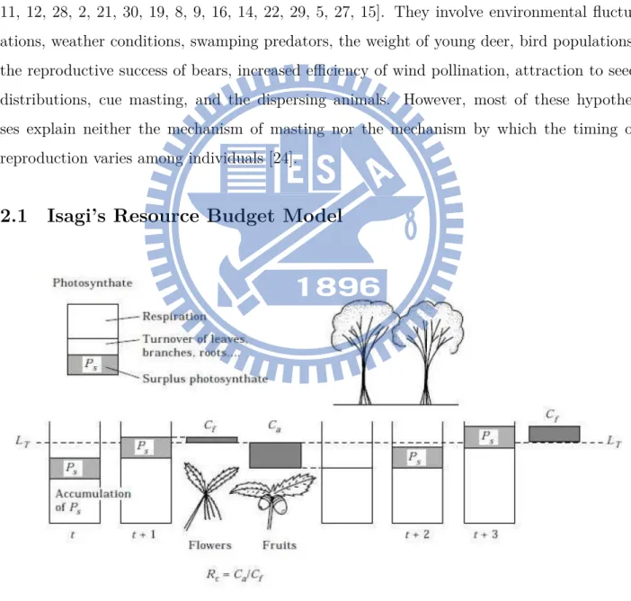
1 Resource budget model of an individual plant. . . 5

2 Phase plane for model (4). . . 8

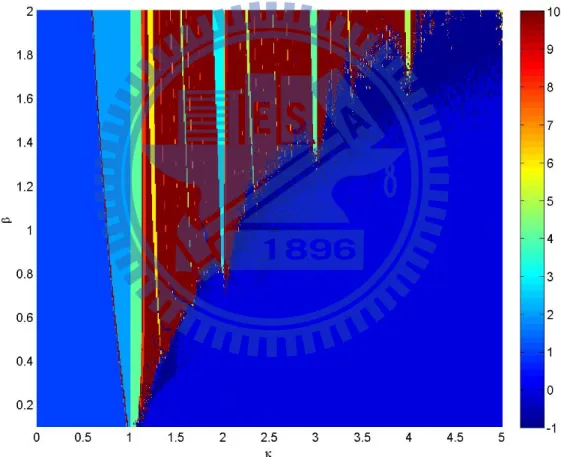
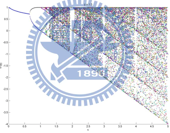
3 Bifurcation diagram for model (6). . . 9

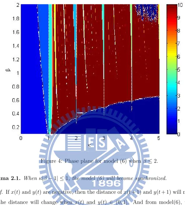
4 Phase plane for model (6) when β ≤ 2. . . 10

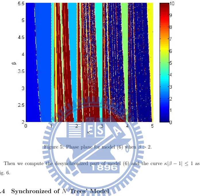
5 Phase plane for model (6) when β > 2. . . . 11

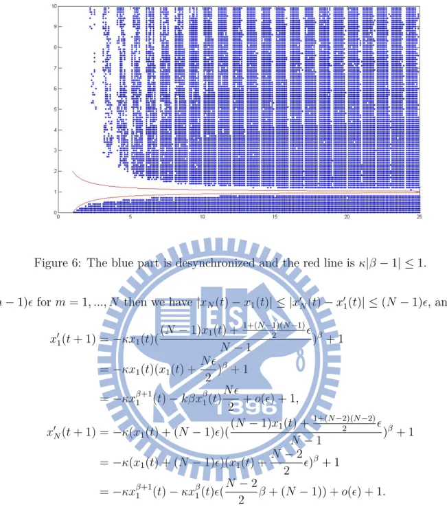
6 The blue part is desynchronized and the red line is κ|β − 1| ≤ 1. . . 12

7 The desynchronized part and curve for 3 trees. . . 13

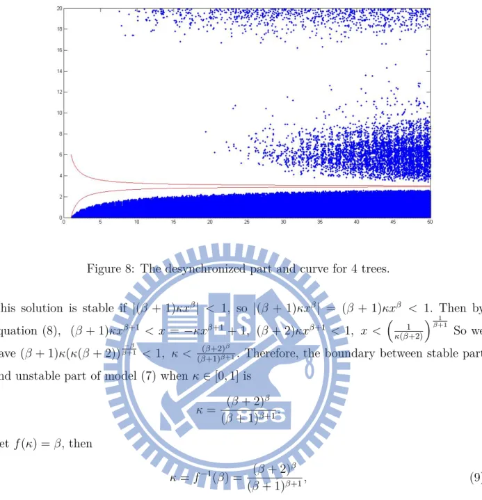
8 The desynchronized part and curve for 4 trees. . . 14

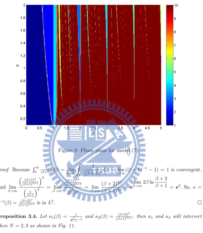
9 Phase plane for model (7). . . 15

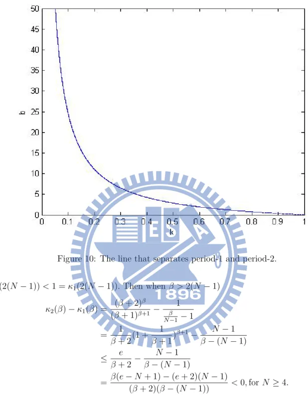
10 The line that separates period-1 and period-2. . . 16

11 The blue line is κ2, and the others are κ1, red is N = 2, cyan is N = 3, green is N = 4, yellow is N = 5. . . . 17

12 The stability for a pair of κ and β. . . . 18

13 The graph of tent map when coefficient is 2. . . 20

14 The graph of model (7). . . 21

15 Lyapunov Exponents of model (6) when β = 2. . . . 23

16 First Lyapunov exponents for a pair of κ and β. . . . 24

17 Second Lyapunov exponents for a pair of k and β. . . . 25

18 Lyapunov exponents and the phase plane of the model (6). . . 26

19 Lyapunov exponents of model (7). . . 27

1 Introduction

In ecology, Satake and Iwasa’s generalized resource budget model that modified from Is-agi et al.’s resource budget model in 2000 [24]. They do many analysis and explaination for the simulation of the model generalized resource budget model. But, there is a strange phe-nomenon that the result will become periodic when depletion coefficient κ is cross to positive integer except for other places when κ > 1. So we guess that is happened by simulation’s conuting error.

In recent decades, chaotic theory has advanced rapidly. Many mathematical tools can be used to measure or describe the “chaotic” conditions. In [4], they has proved that General-ized Resource Budget Model [24] has Devaney’s chaos when the depletion coefficient κ _{∈ N} by snapback repellers. It is contradiction with numerical simulation because of conuting er-ror, like use Matlab to simulate tent map when coefficient is 2. In this thesis we use two mathematical tools, topological entropy and lyapunov exponent, with numerical simulation by Matlab to analysis the generalized resource budget model.

1.1

Definitions of Chaos

The definitions of chaos of Devaney and of Li and Yorke are considered herein because they are fundamental and widely accepted:

Definition 1.1 (Devaney [6]). Let X be a metric space. A continuous map f : X _{→ X is}

said to be chaotic on X if

(i) f is topologically transitive. That is, for any pair of nonempty open sets U, V ⊂ X there

exists k > 0 such that fk_{(U )∩ V ̸= ∅;}

(ii) periodic points are dense in X;

(iii) f has sensitive dependence on initial conditions,meaning that, there exists δ > 0 such

that, for any x∈ X and any neighborhood U of x, there exists y ∈ U and m ∈ N such that _|fm_{(x)− f}m_{(y)| > δ.}

Definition 1.2 (Li and Yorke [18]). Let I be an interval of the real line and f : I → I a

continuous function. f is chaotic if f has an uncountable scrambled set S _{⊂ I which satisfies} the following condition:

(i) for every p, q_{∈ S with p ̸= q,}

lim sup

m→∞ |f m

(p)− fm(q)| > 0 and lim inf

m→∞ |f m

(p)− fm(q)| = 0;

(ii) for every p∈ S and periodic point q ∈ I,

lim sup

m→∞ |f

m_{(p)− f}m_{(q)| > 0.}

The following are two ways to measure the chaos, which is “topological entropy” and “Lyapunov exponents.”

1.2

Topological Entropy

Topological entropy is a quantitative measurement of how chaotic the map is. In fact, it is determined by how many “different orbits” there are for a given map (or flow). To get an intuitive idea of the concept, assume that you cannot distinguish points which are closer together than a given resolution ϵ. Then, two orbits of length n can be so distinguished provided there is some iterate between 0 and n for which they are distance greater than ϵ apart. Let r(n, ϵ, f ) be the number of such orbits of length n that can be so distinguished. The entropy for a given ϵ, h(ϵ, f ), is the growth rate of r(n, ϵ, f ) as n goes to infinity. The limit of h(ϵ, f ) as ϵ goes to 0 is the entropy of f , h(f ). The key idea in this sequence of limits is the growth rate of the number of orbits of length n that are at least ϵ apart [23].

Definition 1.3 ([23]). Let f : X → X be a continuous map on the space X with metric d.

A set S _{⊂ X is called (n, ϵ)-separated for f for n a positive integer and ϵ > 0 provided that} for every pair of distinct points x, y ∈ S, x ̸= y, there is at least one k with 0 ≤ k < n such that d(fk_{(x), f}k_{(y)) > ϵ. Another way of expressing this concept is to introduce the distance}

dn,f(x, y) = sup

0≤j<n

d(fk(x), fk(y)).

Using this distance, a set S ⊂ X is (n, ϵ)-separated for f provided dn,f(x, y) > ϵ for every pair

of distinct points x, y_{∈ S, x ̸= y.}

The number of different orbits of length n (as measures by ϵ) is defined by

r(n, ϵ, f ) = max{#(S) : S ⊂ X is a (n, ϵ)-separated set for f},

where #(S) is the number (cardinality) of elements in S.

We want to measure the growth rate of r(n, ϵ, f ) as n increases, so we define

h(ϵ, f ) = lim sup

n→∞

log(r(n, ϵ, f ))

If r(n, ϵ, f ) = enτ_{, then h(ϵ, f ) = τ ; thus, h(ϵ, f ) measures the “exponent” of the manner in}

which r(n, ϵ, f ) grows with respect to n.

Note that r(n, ϵ, f )_{≥ 1 for any pair (n, ϵ), so 0 ≤ h(ϵ, f) ≤ ∞. Finally, we consider the way} that h(ϵ, f ) varies as ϵ goes to 0 ,and define the topological entropy of f as

h(f ) = lim

ϵ→0,ϵ>0h(ϵ, f ).

Theorem 1.4 ([17]). If a continuous map of the interval has positive topological entropy,

then it is chaotic according to the definition of Li and Yorke.

Definition 1.5 ([33]). Let f (x) be a real-valued function which is defined and finite for all x

in a closed bounded interval a≤ x ≤ b. Let

Γ = x0, x1, ..., xm

be a partition of [a, b]; that is, Γ is a collection of points xi, i = 0, 1, ..., m. With each partition

Γ, we associate the sum

SΓ = SΓ[f ; a, b] =

m

∑

i=1

|f(xi)− f(xi−1)|.

The variation of f over [a, b] is defined as

V = V [f ; a, b] = sup

Γ

SΓ,

where the supremum is taken over all partitions Γ of [a, b]. Since 0 ≤ SΓ < +∞, we have

0≤ V < +∞. If V < +∞, f is of unbounded variation on [a, b].

Example 1.6 ([33]). Suppose f is monotone in [a, b]. Then, clearly, each SΓ equals |f(b) −

f (a)|, and therefore V = |f(b) − f(a)|.

Example 1.7. The total variation of tent map for k = 2 on [0, 1].

t(x) =    kx, if x < 1 2, k(1− x), if x ≥ 1₂. (1)

The invariant set is [0, 1]. And f is monotone in [0,1

2] and [ 1

2, 1], so V (t; [0, 1]) = V (t; [0, 1 2]) +

V (t; [1₂, 1]) = 2. It, together with all its iterates, has constant absolute value of the slope

which therefore gives the variation, that is,

V (tn) = 2n.

Corollary 1.8 ([13]). If f : I _{→ I is a piecewise-monotone continuous map, then} lim n→∞ 1 nlog V (f n_{) = h} top(f ),

where V (fn_{) is total variation of f}n _{in an invariant set I.}

Example 1.9. We use Corollary 1.8 to compute topological entropy of tent map (1) for k = 2.

From Example 1.7 we obtain V (tn_{) = 2}n_{, so}

htop(t) = lim n→∞ 1 n log 2 n_{= log 2.}

1.3

Lyapunov Exponents

In discussing chaos, we referred to Lyapunov exponents which measure the (infinitesimal) exponential rate at which nearby orbits are moving apart.

We want to give an expression for determining the growth rate of the derivative of a function

f : R → R as the number of iterates increases. If |(fn₎′_(x

0)| ∼ Ln, then log(|(fn)′(x0)|) ∼

log(Ln_{) = n log(L), or (}1

n) log(|(f n₎′_(x

0)|) ∼ log(L). In the best situations, the limit of this

quantity exists as n goes to infinity. If we take the limsup, then it always exists as n goes to infinity [23].

Definition 1.10 ([23]). Let f : _{R → R be a C}1 _{function. For each point x}

0, define the

lyapunov exponents of x0, λ(x0), as follows:

λ(x0) = lim sup n→∞ 1 nlog(|(f n )′(x0)|) = lim sup n→∞ 1 nΣ n−1 j=0 log(|f′(xj)|),

where xj = fj(x0). (The first and second limits are equal by the chain rule.) Note that

the right-hand side is an average along an orbit (a time average) of the logarithm of the derivatives.

Remark 1.11. Assume λ(x0) > 0 which implies that

log(|(fn₎′_(x

0)|) ≈ nλ(x0) or |(fn)′(x0)| ≈ enλ(x0) = L(x0)n,

where L(x0) = eλ(x0) > 1, and

|fn

(x0+ δ)− fn(x0)| ≈ |(fn)′(x0)|δ → ∞, as n → ∞.

Therefore, a positive Lyapunov exponent means sensitive dependence on initial conditions, this result is very important and useful since it enables a single quantity to be computed to determine whether a chaotic process is highly sensitive to initial conditions [23, 34].

2 Ecological Models and Numerical Simulation

Many trees in forests reproduce intermittently, rather than at a constant rate [24]. A number of flowers and fruits are produced in a particular year (called a mast year) but very little reproductive activity occurs during several subsequent years until the next mast year. This “synchronous production of highly variable amount of seeds from year to years by a population of plants” is called masting [24]. Perfect periodicity in reproduction is rarely observed, and the intervals between masting are rather irregular.

Several explanations of the masting phenomenon have been proposed [3, 25, 26, 31, 14, 11, 12, 28, 2, 21, 30, 19, 8, 9, 16, 14, 22, 29, 5, 27, 15]. They involve environmental fluctu-ations, weather conditions, swamping predators, the weight of young deer, bird populfluctu-ations, the reproductive success of bears, increased efficiency of wind pollination, attraction to seed distributions, cue masting, and the dispersing animals. However, most of these hypothe-ses explain neither the mechanism of masting nor the mechanism by which the timing of reproduction varies among individuals [24].

2.1

Isagi’s Resource Budget Model

Figure 1: Resource budget model of an individual plant.

that was based on the resource budget of an individual tree [10]. As in Figure 1. From photosynthesis, a mature tree gains net production PS per year, which is accumulated in the

trunk or branches. When the energy reserve exceeds a critical level for reproduction, the tree sets flowers and produces seeds and fruits. Let S(t) be the amount of energy reserve at the beginning of year t. If the sum S(t)+Psis below a critical level Lt, the tree does not reproduce

and saves all the energy reserve for the following year.However, if the sum exceeds Lt, the tree

uses energy for flowering. They assumed that the energy expenditure for flowering is exactly as same as the excess [10], a(S(t) + Ps− LT), in which a is a positive constant. Flowering

plants may be pollinated and set seeds and fruits. It is assumed that the cost for fruits is proportional to the cost of flowers, and is expressed as Rca(S(t) + Ps− LT), in which Rc is

the ratio of fruiting cost to flowering cost. After the reproductive stage, the energy reserves of the tree falls to S(t) + Ps− a(Rc+ 1)(S(t) + Ps− LT). Hence, we have

S(t + 1) =    S(t) + Ps, if S(t) + Ps ≤ LT, S(t) + Ps− a(Rc+ 1)(S(t) + Ps− LT), if S(t) + Ps> LT, (2) (S(t + 1) + Ps− LT) Ps =    (S(t)+Ps−LT) Ps − 1, if S(t) + Ps ≤ LT, (1−a(Rc+1))(S(t)+Ps−Lt) Ps + 1, if S(t) + Ps > LT.

Then introduce a non-dimensionalized variable Y (t) = (S(t)+Ps−LT)/Ps. Then equation (2)

is rewritten as Y (t + 1) =    Y (t) + 1, if Y (t)≤ 0, −κY (t) + 1, if Y (t) > 0, (3)

in which κ = a(Rc+ 1)− 1. The parameter κ indicates the degree of resource depletion after

a reproductive year divided by the excess amount of energy reserve before the year. We call

κ the depletion coefficient, and assume that κ > 0. From equation (3), Y (t) ≤ 1 holds. We

also note that the quantity Y (t) is positive if and only if the tree invests some reproductive activity in year t.

After this rescaling,the dynamics of equation (3) include only a single parameter κ. Other parameter such as the annual productivity Ps or the critical level of reproduction LT do not

affect the essential features of the dynamics if κ remains the same. In [24] and [4], authors proposel many theoretical and numerical results for the model (3). In this thesis , we will focus on the models of two or more trees and introduce the model later.

2.2

Coupling of Trees Through Pollen Availability

In the model described above, when κ > 1, small initial differences in energy reserves between individuals increase with time. This makes it difficult for different trees to synchronize their reproduction. However, synchronized reproduction of trees is often reported in many forests. Fruiting efficiency may depend on the flowering activity of the other trees in a forest because pollination efficiency changes with the number of plants flowering in a population [20]. This effect can lead to the intermittent flowering of trees to become synchronized as shown by the Isagi et al. (1997) computer simulation. Using our notations, pollen coupling can be formalized as follows: consider a forest including N individuals with index i (i = 1, 2, . . . , N ). To model the pollen limitation of reproduction, we replace κ in equation (3) by κPi(t). Pi(t)

is a factor smaller than or equal to 1, and it indicates pollen availability for the i-th tree. Then the non-dimensionalized energy reserve of the i-th tree is

Yi(t + 1) =    Yi(t) + 1, if Yi(t)≤ 0, −kYi(t)Pi(t)β+ 1, if Yi(t) > 0, (4) in which Pi(t) is given by Pi(t) = ( 1 N − 1 ∑ j̸=i [Yj(t)]+ ) , (5)

where [Y ]+ = Y if Y > 0; [Y ]+ = 0 if Y ≤ 0. Pi(t) = 1 holds when all the other trees

reproduce at full intensity (Yj(t) = 1 for all j ̸= i). The smallness of factor Pi(t) indicates the

strength of pollen limitation in seed and fruit production. In calculating pollen availability, Isagi et al. [10] summed up over all the individuals in the forest, but we exclude tree i itself from the sum in equation (5) because only outcrossed pollen is assumed to contribute seed and fruit sets.

The parameter β determines the shape of the function Pi(t) in equation (5) and controls

the degree of dependence of fruit production on outcross pollen availability. If β is close to zero, fruit production is almost independent of the reproductive activity of the other trees in a forest. Small β corresponds to either a high pollination efficiency or a high density of trees because a small fraction of flowering in the rest of the forest is sufficient to achieve good fruiting success. In contrast, a large β implies a strong dependence of seed and fruit production on the reproductive activity of other trees in the forest. Consider a tree that flowers in a year in which only a small fraction of other trees flower. The tree will fail to produce many fruits because of pollen limitation, and it will not experience a heavy resource

depletion. The tree will continue to flower in the following years, until the year comes in which many other trees in the forest also flower at a high blooming intensity. Then they all experience a large fruit set and resource depletion, which gives a mechanism to make different individual trees synchronized in the face of chaotic tendency of each individual. Hence we call β the coupling strength [10].

Then we compute the phase plane of this model as shown in Fig. 2. First we iterate the model for 1500 steps, then to see the situation of the next 1000 steps. Every parts depends on colors according to the color bar indicates the period, and the navy blue part is desynchronized, between the synchronized part and desynchronized part, there is black blue part represents clustering, and red part is high period.

2.3

Two Trees’ Model

In order to analyze this model, first we consider two trees, this way there are not clustering part. So, the model becomes

(Y1(t + 1), Y2(t + 1)) =                (Y1(t) + 1, Y2(t) + 1), if Y1(t)≤ 0, Y2(t)≤ 0, (Y1(t) + 1, 1), if Y1(t)≤ 0, Y2(t) > 0, (1, Y2(t) + 1), if Y1(t) > 0, Y2(t)≤ 0,

(−κY1(t)Y2β(t) + 1,−κY2(t)Y1β(t) + 1), if Y1(t) > 0, Y2(t) > 0.

(6) And the bifurcation diagram of these two trees is shown as Fig. 3. It looks like period doubling, but when k close to nature number, it will become periodic.

Figure 3: Bifurcation diagram for model (6).

Then we compute the phase plane of this model (6) as shown in Fig. 4 and Fig. 5. First we iterate the model for 1500 steps, then to see the situation of the next 1000 steps. In this pair of figures, Every parts depends on colors according to the color bar indicates the period, and the navy blue part is desynchronized. We can see that the model will go into a period cycle when κ cross to _{N. And the width of these periodic parts will become wider when β} become bigger, the first Lyapunov exponent on these parts are also negative.

Figure 4: Phase plane for model (6) when β ≤ 2.

Lemma 2.1. When κ|β − 1| ≤ 1, the model (6) will become synchronized.

Proof. If x(t) and y(t) are negative, then the distance of x(t + 1) and y(t + 1) will not change.

So, the distance will change when x(t) and y(t) ∈ (0, 1]. And from model(6), there exist time t such that y(t), x(t) _{∈ (0, 1]. This way, we suppose in time t, we have x(t) < y(t)}

y(t), x(t) ∈ (0, 1] and they are close. And in time t + 1 they become synchronized. That is,

let x(t) = m, y(t) = m + ϵ, _{|x(t) − y(t)| = ϵ, ϵ is small. Then,}

x(t + 1) =−κm(m + ϵ)β+ 1 =−κm(mβ+ C₁βmβ−1ϵ + o(ϵ)) + 1 =−κmβ+1− κβmβϵ− κm ∗ o(ϵ) + 1, y(t + 1) =−κ(m + ϵ)mβ+ 1 =−κmβ+1− κϵmβ+ 1, |x(t + 1) − y(t + 1)| = |(−κmβ+1_{− κβm}β ϵ− κm ∗ o(ϵ) + 1) − (−κmβ+1− κϵmβ + 1)| =| − κ(β − 1)mβϵ− κm ∗ o(ϵ)| ≈ | − κ(β − 1)mβ ϵ| = κ|β − 1|mβϵ

because mβ _{< 1, we can find a sufficient condition κ|β −1| ≤ 1 such that |x(t+1)−y(t+1)| ≈}

Figure 5: Phase plane for model (6) when β > 2.

Then we compute the desynchronized part of model (6) and the curve κ_{|β − 1| ≤ 1 as} Fig. 6.

2.4

Synchronized of N Trees’ Model

Theorem 2.2. When κ_{|1 −} β

n−1| < 1, the resource budget model (4) with N-trees will

syn-chronized.

Proof. Suppose there are N trees at time t, x1(t), x2(t), ..., xN(t) ∈ (0, 1] such that x1(t) ≤

x2(t) ≤ · · · ≤ xN(t), N ≥ 2. Let ϵ = max

m=2,··· ,N{|xm(t)− xm−1(t)|}, and let xm(t) ′ _{= x}

Figure 6: The blue part is desynchronized and the red line is κ|β − 1| ≤ 1.

(m− 1)ϵ for m = 1, ..., N then we have |xN(t)− x1(t)| ≤ |x′N(t)− x′1(t)| ≤ (N − 1)ϵ, and

x′₁(t + 1) =−κx1(t)( (N − 1)x1(t) +1+(N−1)(N−1)₂ ϵ N− 1 ) β_{+ 1} =−κx1(t)(x1(t) + N ϵ 2 ) β_{+ 1} =−κxβ+1₁ (t)− kβxβ₁(t)N ϵ 2 + o(ϵ) + 1, x′_N(t + 1) =−κ(x1(t) + (N− 1)ϵ)( (N − 1)x1(t) + 1+(N−2)(N−2)₂ ϵ N − 1 ) β_{+ 1} =−κ(x1(t) + (N− 1)ϵ)(x1(t) + N − 2 2 ϵ) β _{+ 1} =−κxβ+1₁ (t)− κxβ₁(t)ϵ(N − 2 2 β + (N − 1)) + o(ϵ) + 1.

Because model (4) is strictly decreasing so _|xN(t + 1)− x1(t + 1)| ≤ |x′N(t + 1)− x′1(t + 1)| ≤

|κxβ 1(t)ϵ(N − 1 − β) + o(ϵ)| ≈ |κx β 1(t)ϵ(N − 1 − β)| = κ|N − 1 − β|x β 1(t)ϵ. And x β 1(t) ≤ 1,

so we can find a sufficient condition κ_{|1 −} β

N−1| < 1 such that |xN(t + 1)− x1(t + 1)| ≤

|x′

N(t + 1)− x′1(t + 1)| ≈ κ|N − 1 − β|x

β

1(t)ϵ < (N− 1)ϵ.

This way we compute the desynchronized part of model (4) and this curve for N = 3, 4 as Fig. 7 and Fig. 8.

So, in order to analyze the behavior of model (4), we rewrite the model as

Y (t + 1) =    Y (t) + 1, if Y (t)_{≤ 0,} −κY (t)β+1_{+ 1, if Y (t) > 0.} (7)

Figure 7: The desynchronized part and curve for 3 trees.

After we rewrite the model, the phase plane become Fig. 9. Instead of Fig. 2’s desynchronized part, the behavior of these two models are almost identical.

3

Mathematical Analysis

The following are some mathematical analysis of Isagi’s resource budget model. We sup-pose the trees are synchronized as model (7).

3.1

Stability Analysis

Suppose F (x) has a period-n solution. If _|(F(n)₎′_{(x)| < 1, then the solution is stable. If}

|(F(n)₎′_{(x)| = 1, then the solution is unstable.}

Corollary 3.1 ([7]). Suppose x0, x1, ..., xn lie on a cycle of period n for F with xi = Fi(x0).

Then

(Fn)′(x0) = F′(xn−1)· · · F′(x1)· F′(x0).

For κ ≤ 1 on the Fig. 2, we can see that this part is fulled by period-1 and period-2. And in the period-1’s district, the solution satisfies

Figure 8: The desynchronized part and curve for 4 trees.

This solution is stable if _{|(β + 1)κx}β_{| < 1, so |(β + 1)κx}β_{| = (β + 1)κx}β _{< 1. Then by}

equation (8), (β + 1)κxβ+1 _{< x = −κx}β+1 _{+ 1, (β + 2)κx}β+1 _{< 1, x <} ( 1 κ(β+2) ) 1 β+1 So we have (β + 1)κ(κ(β + 2))β+1−β < 1, κ < (β+2) β

(β+1)β+1. Therefore, the boundary between stable part

and unstable part of model (7) when κ∈ [0, 1] is

κ = (β + 2) β (β + 1)β+1. Let f (κ) = β, then κ = f−1(β) = (β + 2) β (β + 1)β+1, (9)

f−1(0) = 1, and we show the equation (9) as Fig. 10.

Question 3.2. Does f−1(β) belong to L1_?

Proof. Because ∫₀∞ 1

β+1dβ = lim_t→∞

∫ t

0

1

β + 1dβ = limt→∞(ln(t + 1)− ln 1) = limt→∞ln(t + 1) is

diver-gent. And lim

β→∞ (β+2)β (β+1)β+1 1 β+1 = lim β→∞ (β + 2)β (β + 1)β = e lim β→∞β ln β + 2 β + 1 , lim β→∞β ln β + 2 β + 1 = limβ→∞ lnβ+2 β+1 β−1 = lim β→∞ β+1 β+2 β+1−(β+2) (β+1)2 −β−2 = limβ→∞ β2

(β + 1)(β + 2) = 1, that is, limβ→∞

(β+2)β (β+1)β+1 1 β+1 = e. So, κ = f−1(β) = (β+2)β (β+1)β+1 is not in L 1_.

Figure 9: Phase plane for model (7). Proof. Because ∫₀∞ 1 (β+1)2dβ = lim t→∞ ∫ t 0 1 (β + 1)2dβ = lim_t→∞((t + 1) −1_{− 1) = 1 is convergent.} And lim β→∞ ( (β+1)β (β+1)β+1 )2 ( 1 β+1 )2 = lim_β→∞ (β+1)2β (β+1)2β+2 1 (β+1)2 = lim β→∞ (β + 2)2β (β + 1)2β = e lim β→∞2β ln β + 2 β + 1 = e2 . So, κ = f−1(β) = _(β+1)(β+2)β+1β is in L2. Proposition 3.4. Let κ1(β) = β1 N−1−1 and κ2(β) = (β+2)β

(β+1)β+1, then κ1 and κ2 will intersect

when N = 2, 3 as shown in Fig. 11.

Proof. We know κ1(2(N− 1)) = 1, and (κ2)′(β) =

(β+2)β (β+1)β+1(ln( β+2 β+1)− 2 β+2), because ln( β+2 β+1) = log(1 + 1 β+1) < 1 β+1, so (κ2)′(β) < (β+2)β (β+1)β+1( 1 β+1 − 2 β+2) < 0. And κ2(0) = 1, so we have

Figure 10: The line that separates period-1 and period-2. κ2(2(N − 1)) < 1 = κ1(2(N − 1)). Then when β > 2(N − 1) κ2(β)− κ1(β) = (β + 2)β (β + 1)β+1 − 1 β N−1 − 1 = 1 β + 2(1 + 1 β + 1) β+1₋ N − 1 β− (N − 1) ≤ e β + 2 − N − 1 β− (N − 1) = β(e− N + 1) − (e + 2)(N − 1) (β + 2)(β− (N − 1)) < 0, for N ≥ 4.

(i) When N = 2, choose β = 4, we have κ2(4)≈ 0.4147 > κ1(4)≈ 0.3333.

(ii) When N = 3, choose β = 20, we have κ2(20)≈ 0.1207 > κ1(20)≈ 0.1111.

Therefore, κ1 and κ2 have an intersection on [2,∞) when N = 2, 3 and has no intersection

when N ≥ 4.

In order to look the stability for other κ and β, we use MATLAB to make a figure to show the stability for a pair of κ and β by Corollary 3.1 which is,

|(F(n)

Figure 11: The blue line is κ2, and the others are κ1, red is N = 2, cyan is N = 3, green is

N = 4, yellow is N = 5.

and the equation

F′(x) =    1, x < 0, −(β + 1)κxβ_{, x > 0.}

Then we get a figure as shown in Fig. 12. In Fig. 12, green part represents stable, cyan part represents high period, and navy blue part represents unstable.

Now we let Y (t) = ϵ be the initial value of deviation from Y (t) = 0, and assume that these are small in magnitude. In the next step, Y (t + 1) are slightly smaller or equal to 1, which leads to the conclusion that Y (t + 2) are slightly larger or equal to 1− κ. In the following steps, Y (t + 2) is simply added by 1 per unit time. Hence Y (t + κ + 1) is close to 0 but is positive. This implies that starting from any value close to 0, after κ + 1 steps, Y (t + κ + 1) is small positive.

So, if Y (t) = ϵ, then Y (t + κ + 1) = −κ(−κϵβ+1_{+ 1)}β+1_{+ κ =} −κ(1 + Cβ+1

1 (−κϵβ+1) +

o(ϵβ+1) + κ = κ2(β + 1)ϵβ+1.

And the ratio of |Y (t + κ + 1)| and |Y (t)| is

|Y (t + κ + 1)|

|Y (t)| =

κ2_{(β + 1)ϵ}β+1

ϵ = κ

2_{(β + 1)κϵ}β _{→ 0 as ϵ → 0.}

Figure 12: The stability for a pair of κ and β.

solution (_{−κ + 1, −κ + 2, . . . , 0, 1). From this, we can conclude that this periodic solution is} stable as long as β > 0.

When κ is close to but not the same as an integer, we consider κ is close to 2. The exact periods of these cycles are 3, 6, 12 or still longer one. But the numerical values of all of these cycles are close to a cycle of period 3, being close to 0, 1,-1 and close to 0 again. To examine the exact location of these branches and their local stability, we must calculate each candidate cycle and its stability condition.

So, we first consider period 3 cycle starting from a small positive value. Let Y (t) = ϵ, where ϵ is small positive value. Then Y (t + 1) =_−κϵβ+1_{+ 1, which is close to 1. Y (t + 2) =}

−κ(−κϵβ+1 _{+ 1)}β+1

+ 1, which is close to -1. Y (t + 2) = −κ(−κϵβ+1 + 1)β+1 + 2, which is close to 0. So the period 3 cycle satisfy ϵ = _{−κ(−κϵ}β+1 _{+ 1)}β+1

+ 2, and this equation has positive solution ϵ > 0 if 1.881 < κ < 2 [24]. And this cycle’s stability condition is

| − (β + 1)κϵβ_{|| − (β + 1)κ(−κϵ}β+1 _{+ 1)}β_{| = κ}2_{(β + 1)}2_ϵβ_(−κϵβ+1_{+ 1)}β _{< 1 as ϵ sufficiently}

small.

where ϵ is small positive value. Then Y (t + 1) = _{−ϵ + 1, which is close to 1. Y (t + 2) =}

−κ(−ϵ + 1)β+1

+ 1, which is close to -1. Y (t + 3) = −κ(−ϵ + 1)β+1 + 2, which is close to 0. So the period 3 cycle satisfy_{−ϵ = −κ(−ϵ + 1)}β+1

+ 2, and this equation has positive solution

ϵ > 0 if κ > 2, no positive solution ϵ > 0 if κ ≤ 2. And this cycle’s stability condition is | − (β + 1)κ(−ϵ + 1)β_{|, which cannot be satisfied whether (β + 1)κ(−ϵ + 1)}β _{is bigger or less}

than 1 if ϵ is small because κ is close to 2. So, it is unstable.

And consider period 3 cycle starting from a small positive value Y (t) = ϵ+, comes back

to a small negative Y (t + 3) =−ϵ₋ after 3 steps, and then comes back to the starting small positive value after another 3 steps Y (t + 6) = ϵ+. And this cycle’s stability condition is

| − (β + 1)κϵβ

+|| − (β + 1)κ(−κϵ

β+1

+ + 1)β|| − (β + 1)κ(1 − ϵ−)β|, according to the numerical

analysis, the branch of period 6 is stable for 1.982 < κ < 2.018 but unstable outside of this range [24].

In a similar manner, we can calculate the periodic cycles and its local stability for a longer period.

3.2

Topological Entropy of the Model

By corollary 1.8, if f : I → I is a piecewise-monotone continuous map then lim

n→∞(

1

n log V (f

n_{)) =}

htop(f ) [13].

V (fn_{) is total variation of f}n _{in an invariant set I. In order to compute the total variation,}

we first cut the invariant set into m disjoint parts, and these parts will exactly cover another part or union of some parts through the function. Then we count the number of these parts as the total length of the iteration.

Example 3.5. The total variation of n times iterated of tent map 1 for k = 2.

t(x) =    2x, if x < 1 2, 2− 2x, if x ≥ 1₂.

The invariant set is [0, 1], then we separate I = [0, 1] to I1 = [0,1₂] and I1 = [1₂, 1], t(I1) = I,

t(I2) = I,

V (t(I1)) = V (I) = I1+ I2, V (t(I2)) = V (I) = I1+ I2.

So, V (t0_{) = V (I) = I}

1 + I2, the total length is generated by the length of I1, I2.

the total length is generated by the length of 2I1, 2I2,

V (t2) = 2V (t(I1)) + 2V (t(I2)) = 4I1+ 4I2,

the total length is generated by the length of 4I1, 4I2.

Follow this way, then we distribute a matrix that represent the transition of the quantity of every parts. That is, let T =



 1 1

1 1 

, so we can compute the total variation by

V (tn) = [ V (I1) V (I2) ]  1 1 1 1   n  1 1   =[ 1 2 1 2 ]  1 1 1 1   n  1 1   = 2n_.

From this example, we can see that if we define the graph of the model (as Fig. 13), then we can use this graph to distribute the transition matrix to compute the total variation.

Figure 13: The graph of tent map when coefficient is 2.

Consider the model (7) for κ∈ N, κ ≥ 2, the invariant set is [−κ + 1, 1]. Now we separates this set into κ parts, that is,

I = [−κ + 1, 1] = [−κ + 1, −κ + 2] ∪ [−κ + 2, −κ + 3] ∪ · · · ∪ [−1, 0] ∪ [0, 1] =

κ

∪

m=1

Im,

and by the definition of this model, f (I_m−1) = Im, for m = 1,· · · , κ − 1, f(Iκ) = I,

V (f (Im−1)) = V (Im), for m = 1,· · · , κ − 1, V (f(Iκ)) = V (I) = V (I1) + V (I2) +· · · + V (Iκ).

So, V (f0_{) = V (I) = V} ( ∪ m=1,··· ,κ Im )

= I1 + I2 +· · · + Iκ = κ. Now the total length is

generated by the length of I1, I2, . . . , Iκ. Then V (f1) = V (f (I)) = V

( ∪ m=1,··· ,κ f (Im) ) = V ( ∪ m=1,··· ,κ−1 f (Im) ) + V (f (Iκ)) = (I2+ I3+· · · + Iκ) + (I1+ I2+· · · + Iκ) = I1+ 2I2+· · · +

2Iκ−1+ 2Iκ the total length is generated by the length of 2I1, 2I2, . . . , 2Iκ−1, Iκ.

Follow this way, Then we can distribute a matrix that represent the transition of the quantity of every parts (also can by the graph as Fig. 14).

Figure 14: The graph of model (7). That is, let eκ denotes the vector that (eκ)j = δκ,j, then

T = [ eT 2 eT3 · · · eTn ∑n i=1e T i ]T κ×κ , such that V (fn_{) =}[ V (I1) V (I2) · · · V (Iκ) ] 1×κ Tn(∑n i=1e T i ) = [ 1 1 · · · 1 ] 1×κ Tn(∑n i=1e T i ) = ETn_ET_{, where E =}∑n i=1ei.

Proposition 3.6. If f : I _{→ I is a piecewise-monotone continuous map, and the change}

of the variation of f can be represent as a matrix T , then htop(f ) = log λ1, λ1 > 0, where

λi, i = 1, . . . , n are eigenvalues of T and λ1 >|λm|.

Proof. Because this T is irreducible, so by Perron-Frobenius Theorem [1], there exists λ1 >

0, and λ1 > |λm|, for all m ̸= 1, λ1, . . . , λm are eigenvalues of T. And let v1, . . . , vn are

eigenvectors corresponding to λ1, . . . , λn, then (v1, ET) = Ev1 > 0. Represent ET in the

form ET _{= (Ev}

1)v1+ b, b belongs to eigenspace corresponding to λm , for all m ̸= 1. Now,

V (fn) = ETnET = E((Ev1)λn1v1 + Tnb) = λn1((Ev1)2 + αn), αn tends to 0 as n tends to

infinity. So, htop(f ) = lim n→∞( 1 n log V (f n₎₎ = lim n→∞ ( log(λn 1((Ev1)2+αn)) n ) = lim n→∞ ( log λn 1 n + log ((Ev1)2+αn) n ) = lim n→∞( n log(λ1) + β_n n ) = log λ1 (because βn→ 0 as n → ∞).

Definition 3.7 ([32]). The matrix A =                     0 0 · · · 0 −a0 1 0 · · · 0 −a1 0 1 · · · 0 −a2 · · · · · · · · · · · · 0 0 · · · 0 −ak−2 0 0 · · · 1 −ak−1                     ,

is called the companion matrix of the characteristic polynomial

f (t) = (−1)k(a0+ a1t +· · · + ak−1tk−1+ tk).

By Definition 3.7 the transpose of the matrix Tκ∗κwe obtain before is a companion matrix

with a0 = a1 = · · · = ak−1 = −1, and because T and TT has same eigenvalues, so the

eigenvalues of Tκ×κ satisfies −λκ+ λκ−1+ λκ−2+· · · + λ + 1 = 0.

Proposition 3.8. The topological entropy of model (7) is bigger than 0 for κ∈ N \ {1}.

Proof. Because −λκ_{+ λ}κ−1_{+ λ}κ−2_{+· · · + λ + 1 =} −λκ+1+2λκ−1 λ−1 = 0. Let f (λ) =−λ κ_{+ λ}κ−1₊ λκ−2_{+· · · + λ + 1 =} −λκ+1+2λκ₋₁ λ−1 = −λ κ ₊ λκ₋₁ λ−1, then f (1) = κ− 1 > 0, f(2) = −1 2 < 0,

so by Intermediate Value Theorem, there exists a root in the interval (1, 2).Because f′(λ) =

−κλκ−1₊κλκ−1(λ−1)−(λκ₋₁₎ (λ−1)2 =−κλ κ−1₊ κλκ−1 λ−1 − λκ₋₁ (λ−1)2 =−((1 − 1 λ−1)κλ κ−1₊ λκ₋₁ (λ−1)2) < 0 for

λ > 1, so we know f (λ) is strictly decreasing for λ > 1. More precisely, we suppose the root λ = 2− ϵ then f(2 − ϵ) = −(2−ϵ)κ+1_(2−ϵ)−1+2(2−ϵ)κ−1 = ϵ(2−ϵ)_1−ϵκ−1 = 0 , ϵ(2− ϵ)κ_{− 1 = 0, (2 − ϵ)}κ ₌ 1

ϵ,

κ is increase as ϵ decrease, so the root is close to 2 when κ is sufficiently large.

Therefore, htop(f ) = log λ1 > log(1) = 0.

By Theorem 1.4 and Corollary 1.8, we can obtain that the model (7) is chaotic in Li and Yorke’s sense for κ_{∈ N \ {1}.}

4 Numerical Analysis

By Definition 1.10 to compute the Lyapunov Exponents of two trees’ model (6), first we need to compute ∥Df(x)∥, then the Lyapunov Exponents

λ(x0) = lim sup n→∞ ln_|Dfn_(x 0)| n = lim supn→∞ ∑n−1 j=0 ln|Df(xj)| n , where xj = f j (x0).

We use MATLAB to compute the Lyapunov Exponents of model (6) as shown in Fig. 15, Fig. 16, Fig. 17, and Fig. 18.

Figure 15: Lyapunov Exponents of model (6) when β = 2.

In Fig. 15, fixed β = 2, and red line is the first Lyapunov exponents and blue line is the second Lyapunov exponents, then we can see that the first Lyapunov exponents are almost positive when κ > 1 except κ_{∈ N, and second Lyapunov exponents are negative. In Fig. 16} and Fig. 17, these two figures show that the first and the second Lyapunov exponents for a pair of κ and β, we can see that the second Lyapunov exponents are negative. In Fig. 18, the first subfigure is the first Lyapunov exponents for a pair of κ and β, the second subfigure is the phase plane of the model (6) and the period is corresponding to color bar. This way, we can see more careful that the Lyapunov exponents is negative appear in the period part. Then we compute the Lyapunov exponents of model (7) as shown in Fig. 19, we can also see that the first Lyapunov exponents are negative for κ∈ N, too.

5

Future Work

For κ > 0, when κ _{∈ N, there are period solution there, but except here, this model are} almost high period. And these solutions are stable, Lyapunov exponents are also negative,

Figure 16: First Lyapunov exponents for a pair of κ and β.

but the topological entropy are bigger than 1. We guess this is computer’s numerical error like tent map when κ = 2.

The line κ|1− β

N−1| = 1 for n-trees seperates the region to two parts, which is synchronized

by the sense of contraction and others. If we make the condition looser, like become dispersed in next m− 1 steps and closer at m step. This way we may can seperates the synchronized part and desynchronized part more accurately.

In original model (5), when a tree is bigger than one, and others are smaller than one. Next time this tree will become one until another tree is bigger than one. We think this is not reasonable because if one the other tree spent much time to become bigger than one, this model tell us the first tree will stay one and always wait but not withered. So we think this model can be improved. And some plants can flowering itself like papaya, this means it will not wait other trees until they can produce pollen. This way we rewrite model (4) as

Yi(t + 1) =    Yi(t) + 1, if Yi(t)≤ 0, −κYi(t)Pi(t)β+ 1, if Yi(t) > 0, (10)

Figure 17: Second Lyapunov exponents for a pair of k and β. in which Pi(t) is given by Pi(t) = ( 1 N N ∑ j=1 [Yj(t)]+ ) , (11)

where [Y ]+= Y if Y > 0; [Y ]+ = 0 if Y ≤ 0. Then we compute the phase plane of this model

for two trees as Fig. 20. This is deiiferent as Fig. 4 and the analysis of this model can be an extention of this paper.

Figure 18: Lyapunov exponents and the phase plane of the model (6).

References

[1] V. Afraimovich and S.-B. Hsu. Lectures on chaotic dynamical systems. AMS/IP studies

in advanced mathematics, ISSN, 28:1089–3288, 2002.

[2] C. K. Augspurger. Reproductive synchrony of a tropical shrub: experimental studies on effects of pollinators and seed predations on hybanthus prunifolius (violaceae). Ecology, 62:775–788, 1981.

[3] M. Busgen and E. Munch. The Structure and Life of Forest Trees. Chapman and Hall, London, 1929.

[4] S. M. Chang and H. H. Chen. Applying snapback repellers in resource budget models.

Chaos, 21:043126, 2011.

[5] K. M. Christensen and T. G. Whitham. Indirect herbivore mediation of avian seed dispersal in pinyon pine. Ecology, 72:534–542, 1991.

[6] R. L. Devaney. An Introduction to Chaotic Dynamical Systems, Second Edition. Addison-Wesley, Redwood City, Canada, 1989.

Figure 19: Lyapunov exponents of model (7).

[7] R. L. Devaney. A First Course in Chaotic Dynamical Systems. Addison-Wesley, Redwood City, Canada, 1992.

[8] R. A. Ims. The ecology and evolution of reproductive synchrony. Trends Ecol. Evol., 5:135–140, 1990.

[9] R. A. Ims. On the adaptive value of reproudctive synchrony as a predator-swamping strategy. Am. Nat., 136:485–498, 1990.

[10] Y. Isagi, K. Sugimura, A. Sumida, and H. Ito. How does masting happen and synchro-nize? J. theor. Biol., 187:231–239, 1997.

[11] D. H. Janzen. Seed predation by animals. Ann. Rev. Ecol. Syst., 2:465–492, 1971. [12] D. H. Janzen. Why bamboos wait so long to flower. Ann. Rev. Ecol. Syst., 7:347–391,

1976.

[13] A. Katok and B. Hasselblatt. Introduction to the Modern Theory of Dynamical Systems. Cambridge University Press, 1995.

Figure 20: Phase plane for model (10) when β _{≤ 2.}

[15] D. Kelly and J. J. Sullivan. Quantifying the benefits of mast seeding on predator satiation and wind pollination in chinochloa pallens (poaceae). Oikos, 78:143–150, 1997.

[16] R. G. Lalonde and B. D. Roitberg. On the evolution of masting behaviour in trees: predation or weather? Am. Nat., 139:1293–1304, 1992.

[17] S. Li. ω -chaos and topological entropy. transactions of the american mathematical society. 339:243–249, 1993.

[18] T. Y. Li and J. A. York. Period three implies chaos. American Mathematical Monthly, 82(10):985–992, 1975.

[19] E. Matthysen. Nuthatch sitta europaea demography, beech mast, an territoriality. Ornis

Scand, 20:278–282, 1989.

[20] S. G. Nillson and U. Wagstliung. Seed predation and cross-pollination in mast-seeding beech (fagus sylvatica) patches. Ecology., 68:260–265, 1987.

[21] S. G. Nilsson. Eological and evolutionary interactions between reproduction of beech fagus sylvativa and seed eating animals. Oikos, 44:157–164, 1985.

[22] D. A. Norton and D. Kelly. Mast seeding over 33 years by dacrydium cupressinum. lamb. (rimu) (podocarpaceae) in new zealand: the importance of economies of scale. Funct.

Ecol., 2:399–408, 1988.

[23] C. Robinson. Dynamical Systems: Stability, Symbolic Dynamics, and Chaos, Second

Edition. CRC, Boca Raton, Florida, 1998.

[24] A. Satake and Y. Iwasa. Pollen coupling of forest trees: Forming synchronized and periodic reproduction out of chaos. J. theor. Biol., 203:63–84, 2000.

[25] W. M. Sharp and H. H. Chisman. Flowering and fruiting in the white oaks. i. staminate flowering through pollen dispersal. Ecology., 42:365–372, 1961.

[26] W. M. Sharp and V. G. Sprague. Flowering and fruiting in the white oaks: pistillate flowering, acorn development, weather, and yields. Ecology.

[27] M. Shibata, H. Tanaka, and T. Nakashizuka. Causes and consequences of mast seed production of four cooccurring carpinus species in japan. Ecology, 79:54–64, 1998. [28] J. W. Silvertown. The evolutionary ecology of mast seeding in trees. Biol. J. Linnean

Soc., 14:235–250, 1980.

[29] C. C. Smith, J. L. Hamrick, and C. L. Kramer. The advantage of mast years for wind pollination. Am. Nat., 136:154–166, 1990.

[30] T. J. Smith. Seed predation in relation to tree dominance and distribution in mangrove forests. Ecology, 68:266–273, 1987.

[31] V. L. Sork, J. Bramble, and O. Sexton. Ecology of mast-fruiting in three species of north american deciduous oaks. Ecology., 74:528–541, 1993.

[32] Arnold J. Insel Stephen H. Friedberg and Lawrence E. Spence. Linear Algebra. Prentice-Hall, Inc., Englewood Cliffs, New Jersey, 1987.

[33] R. L. Wheeden and A. Zygmund. Measure and Integral. Marcel Dekker, Inc., Madison Avenue, New York, New York, 1977.

[34] Rodeny C. L. Wolff. Local lyapunov exponents: Looking closely at chaos. Journal of the