行政院國家科學委員會專題研究計畫 期中進度報告
平衡計分卡各構面相關性及其影響因素之整體研究─多種
研究方法之運用(1/3)
計畫類別: 個別型計畫 計畫編號: NSC91-2416-H-004-022-執行期間: 91 年 08 月 01 日至 92 年 07 月 31 日 執行單位: 國立政治大學會計學系 計畫主持人: 吳安妮 報告類型: 精簡報告 處理方式: 本計畫可公開查詢中
華
民
國 92 年 7 月 2 日
期中報告(第一年):
第一年之研究方向主要探討與”員工獎酬及員工績效”
有關之研究議題為主
The Impact of Government Intervention on Employee
Compensation Plans and Employee
Performances—An Empirical Study of A Car
Dealership
ABSTRACT
This study reports that in response to government regulations, changes in compensation from performance-sensitive (commission-based) to less performance-sensitive (base salary plus commission) schemes hurt employee performance but do not impair the company’s. We analyzed performance data for 4,392 employees and 87 branches of a major Taiwanese car dealership over 56 months to test how the switch in compensation plan affects individual and firm performance. We find that individual sales productivity, especially that of
high-performance salespersons, decreased once the compensation plan changed. Consistent with the predictions of selection effects, our results indicate that the less
performance-sensitive plan retained fewer high-performance salespersons and recruited more low-performance sales staff. Interestingly, our findings show a deviation from optimal practices as imposed by the government.
Key Words: compensation scheme, government regulations, incentive effect, and selection
1. Introduction
A performance-based incentive plan can motivate people to increase their efforts and can be an effective vehicle to direct management behavior (Kaplan and Norton, 1996; Bonner et al., 2000). While companies may voluntarily change their compensation plans to better motivate their employees, they must comply with government regulations (e.g., minimum wage requirement). Prior management accounting and economic studies (Waller and Chow, 1985; Lazear, 2000; Banker et al., 2001) have examined only a voluntary change in incentive plans (e.g., from hourly wages to piece rates) and have reported that such a change causes an increase in employees’ compensation and improvement in their
performance. Unlike prior studies, this study is one of the first to empirically examine how government intervention in employee compensation plans affects employee sales
productivity and branch performance.
To protect worker rights and interests, in 1998, the Taiwanese Labor Law amendment required that companies give minimum wage (around $466) for all forms of employee-employer relationships and that all implementations be completed by the end of 1998. To comply with the government regulations and also to consider other factors, our research company changed its employee compensation plans from commission-based to base salary plus lower commission rates. Therefore, compared to the old commission-based compensation plan, the new one is less performance sensitive because of lower commission rates. Our empirical evidence shows that changes in the compensation plan result in a decrease in average individual productivity and compensation but an increase in company performance, which is a deviation from optimal practices as imposed by a government entity.
To further explore the effects of compensation plan change, we identify the
employee groups (e.g., high-performance vs. low-performance) most and least affected by the change to a less performance-sensitive compensation plan and whether the impact of such a change is instantaneous or increases over time. Furthermore, economic theories of compensation predict that switching from a performance-sensitive to a less
performance-sensitive compensation scheme will not only evoke a negative incentive effect (i.e., diminish the incentives of employees to exert effort) but also will have selection effects (i.e., attract low-performance and deter high-performance employees), impairing overall company health (e.g., Waller and Chow, 1985; Lazear, 2000; Banker et al., 2001). Therefore, we also have examined how the change to a less performance-sensitive compensation plan affects the company’s recruitment and retention of high- and low-performance employees. Furthermore, we explore how overall company performance is affected by the compensation plan change and what actions management may take to mitigate losses from lower
individual sales productivity.
Our database includes 4,392 detailed, individual-level data (e.g., salespersons’ compensation, sales quantities, and demographic information), branch-level data (e.g., revenues and gross profits) and firm-level data (e.g., turnover rates, new hires) for a period of 56 months. We have run panel data with fixed models and regression models to examine how the change in compensation schemes from performance-sensitive to less
performance-sensitive has affected salespersons’ productivity and attraction to the company. Interestingly, our results show that while the switch in compensation plan worsens
individual performance and compensation, the branch’s financial performance improves. This improved performance may be partly due to the dealership’s hiring more salesmen to
mitigate losses in individual employee performance and also due to their implementation of a low performance improvement plan. Our findings also indicate that the impact has been greater for high-performance than for low-performance salespersons and such an impact grows over time. Furthermore, the less performance-sensitive plan appears to have attracted more low-performance salespersons to the company and retained fewer high performers.
The remainder of this paper is organized as follows: Section 2 describes the research site and the nature of the changes made in the employee compensation plan; Section 3 reviews related prior studies as the bases for developing our hypotheses; data and empirical models follow in Section 4; Section 5 presents empirical results; and Section 6 summarizes our results with concluding remarks.
2. Research site
Over the past few years, Taiwan’s domestic automobile market has been nearly 400,000 cars per year.1 The research site is the largest car dealership there. In 2001, it had
1,248 sales representatives and 87 sales outlets located all over Taiwan and in some parts of Mainland China.
We chose the dealership for three reasons: (1) the dealership had changed its compensation scheme from a performance-sensitive (commission-based) plan to a less performance-sensitive (base salary plus lower commission rates) that conforms to the Law’s requirements. (2) As mentioned, the company is the largest dealership in the automobile market, with nearly 18 percent of market share over the past five years, and attained an ISO 9002 certification in 1999. These facts demonstrate the dealership’s commitment to quality improvement. (3) The dealership agreed to provide us with an archival database containing
4,392 sales representatives and 87 branches over a 56-month period, and the top
management also allowed us access to most internal documents and interviews with their managers and sales forces, if needed. The double availability of this rich database and research resources allowed us to test predictions empirically, based on analytical models of economic theories.
In early 1998, the Taiwanese Labor Law Amendment required minimum wage for all forms of employee-employer relationships. To comply with the Law’s requirement of paying base salary to all employees, the company had to change its commission-based compensation plan, which had functioned very well. The CEO was considering two alternatives: Plan A (adding base salary with the same commission rates) and Plan B (adding base salary with lower commission rates). The idea of lowering commission rates arose from the CEO’s inability to predict the impact of the compensation plan change on company’s revenue and also from the need to control total compensation expenses by having employee compensation be equal under both old and new compensation plans. However, the CEO was not satisfied with either Plan A or Plan B, since the former could hurt the company’s profitability and the latter could hurt employee productivity and cause the company to lose high performers to its competitors.
At that time, the CEO heard that some of their competitors would superficially comply with the Law’s requirement by providing a base salary and maintaining the same commission rates. However, they would demand a penalty⎯the base salary would be taken away from those not meeting the minimum sales requirement. It has been known that the Taiwanese government has not strictly enforced all the regulations promulgated and the penalty associated with companies’ failure to comply with the regulations is not severe.
Therefore, the CEO faced a dilemma: to either comply with the Law’s requirement or to superficially comply with the Law’s requirement and later face government investigation and penalty. On July 1, 1998, after considering all the factors, the CEO decided to comply with the government regulations by adopting Plan B—paying base salary with lowered commission rates—as its new compensation plan for all levels of salespersons. Also, the implementation was throughout the company rather than on a regional or step-by-step basis.
Furthermore, the dealership introduced an Improvement of Low Performance Plan. That is, if a salesperson cannot attain the minimum requirement (nine cars every three months, and then, given the economic downturn in 2001, changing to seven cars every three months), he/she receives an initial warning. If the salesperson cannot improve performance in the following two months, he/she will be forced to quit except for some extenuating circumstances.2
3. Hypotheses development
The premise of agency theory is that a principal designs a contract to direct an agent’s actions in alignment with the principal’s best interests (e.g., Holmstrom, 1979; Feltham and Xie, 1994; Prendergast, 1999; Lambert, 2001). The primary focus of classic models in agency literature has been how to design performance-based contracts to motivate employee effort (incentive effect) (e.g., Milgrom and Roberts, 1992; Banker et al., 1996; Lazear, 2000; Banker et al., 2001). Furthermore, studies have shown that compensation contracts attract and retain high performers and differentiate high from low performers (selection effects) (e.g., Milgrom and Roberts, 1992; Lazear, 2000; Banker et al., 2001). Below, we discuss both incentive and selection effects and the hypotheses to be tested.
2 The research company refused to share with us documents revealing who had not met the minimum sales requirement and been forced to leave the company. We were told that branch managers normally make an
3.1. Incentive effect
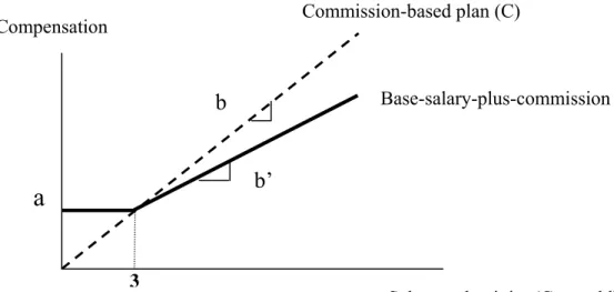
Agency theory maintains that compensation contracts make prescriptions regarding the circumstances under which fixed (base salary) and variable (commissions and other forms such as bonuses or options) components can better align employer and employee interests. For example, suppose, in a commission-based compensation plan, linear
individual compensation contracts of the form C = bx, where b is commission rate and x is productivity or output. Under this contract, C is very sensitive to both x and b. Therefore, employees have incentives to work hard to earn more compensation. Now, assume the company changes compensation plan C to a new one with base salary and lower commission rates. Linear individual new compensation contacts of the form C’ = a + b’x, where a is base salary, b’ is the new commission rate, and b’ < b. When x ≤ 3 (due to the requirement of the Improvement of Low Performance Plan), C’ is equal to a and b’=0 (no commission). That is, employees who sell less than three cars per month receive only base salary. However, when x > 3, employees receive both base salary and commission, depending on their sales productivity. A lower b’ may induce less effort from employees to work hard, resulting in
C’ < C. The graphical presentations of the two compensation contracts C and C’ are
summarized in Figure 1.
_________________________ Insert Figure 1 about here __________________________
The notion that performance-based incentives affect employee behavior is evidenced in several empirical studies (e.g., Banker et al., 1996; Bailey et al., 1998; Lazear, 2000). Banker et al. (1996) reported that implementing a performance-based compensation plan
increased sales and that the effect persisted and grew over time. Bailey et al. (1998) found that improvement rates in individuals’ initial and overall performances of an assembly task are higher when an incentive plan is in place. Similarly, Lazear (2000) examined the impact of piece rates on the performance of workers who install auto windshields. He found that worker output increased after the company switched its compensation scheme from hourly wages to piece rates.
In contrast to the empirical evidence discussed above, experimental studies have reported mixed findings on how incentives affect performance. Ashton (1990) concluded that auditors’ bond-rating performance in the “incentive plus feedback” condition was not significantly better than their counterparts’ in the “feedback only” condition. Conversely, Sprinkle (2000) reported that participants receiving an incentive-based contract performed better on a production decision task than those who received a flat-wage contract. Also, the rate of performance improvement increased when participants either spent more time working on the task or analyzed the provided information more thoroughly. Sprinkle also pointed out that participants’ initial performance on a cognitive task is not very sensitive to the increased effort induced by incentives, but their subsequent performance improvement is.
Lazear (2000) argued that workers in a performance-sensitive situation tend to exert more effort to be productive. That is, a company switches from contract C
(performance-sensitive plan) to contract C’ (less performance-sensitive plan) will induce less effort from employees, which will, in turn, reduce their productivity. These arguments lead to our first hypothesis:
H1: Employees’ average sales productivity (cars sold) will decrease after the company changes its compensation plan to a less performance-sensitive
scheme.
Figure 1 shows the relationship between compensation and cars sold under both the
C and C’ compensation schemes. Clearly, when sales productivity increases, the differences
in compensation under these two schemes increase. This suggests that switching from compensation plan C to C’ will cause high-performance employees to lose more benefits (due to lower commission rates) than low-performance employees, and the poorest performers may actually gain the most (with a guaranteed base salary). Furthermore, compared to low-performance employees who meet a minimum requirement of sales productivity, high-performance employees will have less incentive to work harder. This results in comparatively lower sales productivity. These arguments lead to the following hypothesis:
H2: The decrease in sales productivity (cars sold) of high-performance employees after a company changes to a less performance-sensitive compensation scheme will be greater than that of low-performance employees.
Agency models typically assume that employees have perfect knowledge of their individual abilities. In reality, employees may not have concrete knowledge of their own abilities nor of the impact of the compensation plan change on their individual compensation. They may learn about these over time as they receive feedback on their performance and compensation. Therefore, when a change in compensation plan is made from C to C’, the impact on the workforce’s composition may not be instantaneous. Employee turnover is likely to continue for several periods after plan implementation, and organizational
productivity is expected to grow progressively higher over time (Banker et al., 2001, p. 321). This argument is supported by previous findings that the longer the salespersons are under the more performance-sensitive plan, the higher the impact on sales productivity (Lazear,
2000; Sprinkle, 2000; Banker et al., 2001). By analogy, we expect that the longer the less performance-sensitive compensation scheme C’ has been in effect, the more negative impact on individual sales productivity. Therefore, we propose the following hypothesis:
H3: Under the less performance-sensitive compensation plan, the negative impact on employees’ sales productivity (cars sold) will increase over time.
3.2. Selection effects
Companies design compensation schemes not only to induce more employee effort but also to attract potential employees. Recent studies suggest that performance-based incentive plans effectively sort employees by ability (Lazear, 2000; Banker et al., 2001). Selection effects include recruiting and separation effects. The former relates to the type of employees who join the company, and the latter to the type of employees who leave it. Lazear (2000) showed that contracts with higher piece rates attract high-ability employees. In a review paper, Prendergast (1999) argued that compensation contracts are important means for a company to recruit more capable workers, since they will benefit more from a performance-sensitive compensation plan than the less capable will. In turn, the more capable will be more likely to be attracted to the company than the less capable, therefore the company will have a higher percentage of high performers.
Conversely, when a company switches compensation schemes from C to C’, it is likely that the guarantee of a base salary will attract more low-performance employees. Therefore, the recruiting effect suggests that the sales productivity of employees hired after the switch to contract C’ will be lower than that of those hired before the plan switch. These arguments lead to the following hypothesis:
H4: The average sales productivity (cars sold) of employees hired under the less performance-sensitive compensation scheme will be less than that of
Hollenbeck and Williams (1986) pointed out an important distinction between the frequency and functionality of turnover. While the former refers to the number of turnover separations, the latter refers to the implication for an organization of those separations. A company benefits when low-performance employees leave, but it suffers a setback when high-performance employees leave. Thus, it is important to consider who will leave the company when there is a switch from a C scheme to a C’ scheme.
Using a meta-analysis of 55 studies, Williams and Livingstone (1994) reported that poorer performers tended to leave when pay was based on performance and to stay when pay was not so based. The implication of their findings is that performance-based compensation plans can lead to functional turnover. Lazear (2000) reported that about one-third of
improved performance can be attributed to selection effects, i.e., less productive workers leave the company and are replaced by more-productive workers. In Banker et al. (2001), results showed that a performance-based scheme in a retail firm attracted and retained more productive salespersons, while the performance of the less productive sales staff declined before they left.
Feedback on compensation could help employees learn how they are affected by a less performance-sensitive compensation plan. High-performance employees who
continually compare their compensation with past levels and outside opportunities are likely to be dissatisfied with their compensation. Therefore, the separation effect predicts that high-performance employees are more likely to leave the company, reflecting their
disappointment with the compensation received under the less performance-sensitive plan. Therefore, we expect that the sales productivity of employees who left after the change in compensation scheme from C to C’ to be higher than that of employees who left before the
switch occurred. Below, we propose the following hypothesis concerning separation effects: H5: The average sales productivity (cars sold) of employees who leave under the less
performance-sensitive compensation scheme will be higher than that of employees who leave under performance-sensitive compensation.
4. Model development
4.1. Data
There are 97,541 person-months and 5,121 branch-months of data covered by the 56-month period from January 1996 to April 2001. We partitioned the sample into two sub-samples: (1) before the switch to the new plan (a total of 28 months—from January 1996 to April 1998),3 and (2) after the switch to the new plan (a total of 28 months—from January
1999 to April 2001). We used these two sub-samples to test related hypotheses comparing sales productivity of employee and branch performance before and after the switch to the new plan (PLAN). PLAN is equal to 1 if the salesperson was on the new plan during the given month. We measure employee sales productivity (INDSALE) as number of cars sold per person-month and the branch performance as branch monthly number of cars sold (BSALE), revenue (BREVENUE), gross profit (BGSPROFT), and income before allocating operating expenses of headquarters and income tax (BINCOME).
To identify the employee groups most and least affected by the compensation plan change, we construct a dummy variable ABILITY as a surrogate for employee ability or performance. ABILITY is equal to 1 if the average sales quantity of 1995 is greater than median, 3; otherwise it is 0.4 To evaluate the impact of the change in compensation plan
over time, we construct a variable PLANTIME that measure the number of months from the
3 We excluded eight months (May to December) of 1998 from our sample in order to control both the transition-period and seasonal-month-sales effects.
4 We averaged employees’ sales quantities for the 12 months prior to January 1996, when our sample period started. However, we averaged his/her sale productivity in our data if an employee joined the dealership during this 12-month period.
beginning of the new plan a salesperson was on to the end of our sample period (April 2001). Also, we tested selection effects by examining differences in the performance of those who were hired before and after the switch and also of those who had left the dealership. We classify each employee in our sample as follows:
(1) OLD (DOLD =1, 0 otherwise): Salespersons who had joined the dealership before the switch to the new plan.
(2) OLDQB (DOQB =1, 0 otherwise): Salespersons who had joined the dealership before the switch to the new plan and left before July 1, 1998.
(3) OLDQA (DOQA =1, 0 otherwise): Salespersons who had joined the dealership before the switch to the new plan and left after July 1, 1998 but before the end of our sample period.
(4) NEW (DNEW =1, 0 otherwise): Salespersons who had joined the dealership after the switch to the new plan.
(5) NEWQA (DNQA =1, 0 otherwise): Salespersons who had joined the dealership after the switch to the new plan and left after July 1, 1998, but before the end of our sample period.
4.2. Estimation model
We estimated the models’ parameters using pooled time-series data over a 56-month period and cross-sectional data for the 4,392 individuals and 87 branches. The hypothesized incentive effects of the compensation plan change on sales quantities are tested by
examining coefficients in panel data with fixed effects models 1, 2 and 3. This is because repeated observations on the same set of cross-section units (Johnston and Dinardo, 1997, p.388). We specify the first three models as follows:
it 0 1 it 1 t 2 t
11
3 it mt 1
m 1
INDSALE PLAN LOGFCOMP LOGNFCOMP
LOGCITYS M
=
= α + α + λ + λ
INDSALEit = α0 + α1 PLAN it + β1 ABILITYit + β2 ABILITYit × PLAN it (2) 11 2 t 3 it mt 2 m 1 LOGNFCOMP LOGCITYS M = + λ + λ +
∑
ξ + εINDSALEit = αit0 + ω PLAN0 1 TIMEit it+λ1LOGFCOMP2 t it + λ2LOGNFCOMP3 it (3)it
3L O G C IT Y Sit 3
+ λ + ε
i=1-4,392, a subscript to denote employee i, t=1-56, a subscript to denote the time-period in
which the employee works, andεit is a random error term. In our models 1, 2, and 3, we include two types of control variables, i.e., competition types and competition intensity, to capture the general economic condition. In Taiwan, it is common for car manufacturers to arrange exclusive dealership with distributors, an agreement which prohibits the dealer from selling competing makes (brands). There are two types of competitors to our research company: family competitors (FCOMP) that sell the same brand of cars, and non-family competitors (NFCOMP) that sell different car brands but compete for the same customer groups. We use CITYS (i.e., market monthly sales of competitors located in the same city) as a proxy for competition intensity. The log forms of monthly car sales for FCOM, NFCOM in the Taiwanese market and that of CITYS are included in our models.
When a car dealership launches a new car model, it attracts consumers’ attention, which results in increased sales productivity that normally lasts for several months. Also, there may be seasonal monthly sales effects. Therefore, we include month dummies, Mmt,
in all models except for those having PLANTIME. Furthermore, because of a positive correlation between PLAN and PLANTIME (Pearson r = 0.8145), we have included only PLANTIME in Model 3 to avoid potential multi-collinearity problems.
Recall that this study explores how the compensation plan switch affects all employees, rather than individuals. Therefore, we did not include in Model 1 employees’
personal characteristics, such as experience and ability. Furthermore, since the fixed-effects model using panel data assumes that differences across salespersons can be captured in differences in the constant term (Greene, 2000, p.560), we did not include a variable for experience in Models 2 and 3.
However, the fixed-effects model using panel data is not feasible for testing selection effects, because there was a high employee turnover rate, with some employees leaving the dealership and new entrants joining it at the same time. Consequently, we specify the following regression models 4 and 5 to test hypothesized selection effects:
NEW
it 0 1 it NEW 1 t
11
2 t 3 it mt 4
m 1
INDSALE EXPR r D LOGFCOMP
LOGNFCOMP LOGCITYS M = = α + β + + λ + λ + λ +
∑
ξ + ε (4) NQA OQA it 0 1 it NQA OQA 1 t 11 2 t 3 it mt 5 m 1INDSALE EXPR r D r D LOGFCOMP
LOGNFCOMP LOGCITYS M
=
= α +β + + +λ
+λ +λ + ξ
∑
+ε (5) Model 4 tests the recruiting effect, i.e., comparing the sales productivity of OLD and NEW groups. Model 5 tests separation effects, therefore only employees who had left thedealership (i.e., DOQB, DOQA, and DNQA) are included. In both Models 4 and 5, we do not
include ABILITY or PLAN, nor their interaction variable, because in these models we test only the differences between the groups NEW and OLD. However, we include EXPR (number of months employed) as a control variable since the NEW and OLD groups had different times of employment and separation.
4.3. Tests of hypotheses
Recall H1, which predicts that changing to a less performance-sensitive plan will result in employees’ decreased sales productivity. We test H1 by examining the coefficient of PLAN (α1) of Model 1, and we predict α1 will be negative to indicate a decreased
magnitude of the negative impacts on sales productivity is higher for high-performance salespersons than it is for low-performance salespersons. As H2 predicts, the coefficient of ABILITY × PLAN, β3, should be negative to indicate a larger negative impact on the high-performance employees. As suggested by Banker et al. (2001), employees may learn about their ability and compensation levels over time by receiving feedback on their
performance. Therefore, as H3 predicts, the negative impact on employee sales productivity increases over time, thus the coefficient of PLANTIME, ω, in Model 3 is to be negative.
To test the recruiting effect (H4), we test whether sales productivity of NEW is lower than that of OLD. To avoid for potential multi-collinearity problems, we include only DNEW
in Model 4. The average sales productivity of DOLD is α0, and the average sales productivity
of DNEW is α0+γNEW. Thus, H4 is tested by examining the following inequality: (α0+γNEW) -α0
= γNEW < 0.
To test separation effects (H5), we compare differences in the sales productivity of those who had left before the change in compensation plans (OLDQB) with those of employees who had left after the switch (OLDQA, NEWQA). First, we compare the sales productivity of OLDQB and OLDQA, both groups joined the dealership before the new plan, but they differed in the time of separation. As predicted by H5, the average sales
productivity of OLDQB was less than that of OLDQA. In other words, the coefficient of DOQA (α0+
γ
OQA) is predicted to be greater than that of DOQB (α0) orγ
OQA is greater than zero.Second, we compare the sales productivity of OLDQB with that of NEWQA, both differ not only in their time of joining the dealership but also in their time of separation. Recall that the dealership implemented an Improvement of Low Performance Plan. Therefore, NEWQA includes both poorer performers being forced out and high performers who were not
satisfied with the compensation plan and thus left the dealership. As discussed earlier, we expect the average sales productivities of NEWQA to be better than those of OLDQB or the coefficient of DNQA (α0+
γ
NQA) is greater than that of DOQB (α0) or thatγ
NQA is greater thanzero.
5. Results
5.1. Descriptive statistics
Table 1 summarizes the descriptive statistics of the dealership’s key variables. Means (standard deviations) of the key variables for the whole period and two sub-sample periods are presented in Panel A of Table 1. The average number of cars sold per month per employee is 3.30, which is slightly higher than 3: the minimum requirement under the Improvement of Low Performance Plan. The turnover rate per month is 2.31 percent (or 27.45% per year). This high turnover rate suggests that the composition of the employee workgroup has changed and we are able to examine selection effects.
__________________________ Insert Table 1 about here __________________________
As seen from Panel A of Table 1, the average of INDSALE after the plan switch (3.15) is significantly lower than that before the plan switch (3.49), suggesting that the change to a less performance-sensitive compensation plan decreased individual salesperson productivity. The variance of INDSALE also decreased after the change in compensation plans (from 4.09 to 3.45). This may be attributable to the departure of more
high-performance salespersons and/or to the dealership’s Improvement of Low Performance Plan, which forces the poorest performers to leave the company. Furthermore, the monthly employee turnover rates rose from 2.19 to 2.41 percent, but the difference is not statistically
significant (t= -1.01, p=0.3152).
Figure 2 displays the monthly average sales productivity of different employee types from July 1998 to April 2001. As seen in Panel A of Figure 2, the average sales productivity of OLD is better than that of NEW, suggesting the less performance-sensitive plan attracts more low performers to the firm. Furthermore, Panel B of Figure 2 shows that the sales productivity of OLDQA is higher than that of OLDQB, implying more high performers left the firm after the plan switch. Interestingly, it shows that in general the average sales productivity of NEWQA is below 3 cars over the 34-months period, which shows that the Improvement of Low Performance Plan was effective and that poor performers had to leave the dealership.
In contrast to decreased individual salesperson productivity after the switch to the new compensation plan (from 3.49 to 3.15 cars), Panel A of Table 1 shows an improvement in all branch performance measures (i.e., BREVENUE, BGSPROFT, BINCOME, and BSALE). We will discuss branch performance in detail later. Note that there is a decrease in the company’s market share after the plan switch (from 18.2% to 17.0%); however, it is not statistically significant.
Panel B of Table 1 presents distributions of individual sales productivity for both before- and after-the-plan-switch periods. As shown in Panel B of Table 1, the change to a less performance-sensitive plan caused a decrease in sales productivity. For example, more salespersons sold no car each month after the plan switch (24.8%) than they had before the plan switch (20.1%). Similarly, there is a slightly higher percentage of salespersons who sold less than three cars under the new plan than under the old plan (46.1% vs. 45.2%). Regarding the high performers, after the plan switch there was a decrease in the percentage
of those who sold six or more cars per month (from 20.6% to 17.3%) and also a slight decrease in percentage of those who sold ten or more cars per month (from 4.5% to 3.4%).
5.2. Tests of incentive effect (H1, H2, and H3)
Panels A and B of Table 2 show the panel data and regression results with individual sales productivity as the dependent variable. As seen in Panel A of Table 2, the coefficient of PLAN in Model 1, -0.370, is statistically significant (p < 0.0001). Thus, our results support H1: employees’ average sales productivity decreased after the plan switch.
____________________________ Insert Table 2 about here ____________________________
Regarding H2, Table 2 shows that except for the coefficient of LOGNFCOMP in Model 2, all the coefficients are statistically significant (with p values less than 0.0001). The positive coefficient of ABILITY also suggests that sales productivity is significantly influenced by an employee’s ability. Consistent with the prediction of H2, the coefficient of ABILITY × PLAN of Model 2 has a negative sign (-1.669). The negativity of the sign suggests that under the less performance-sensitive compensation plan, the sales productivity of high-performance salespersons decreased more than that of low-performance sales staff. Thus, our result supports H2.
Recall that H3 predicts there is an increasingly negative impact on employees’ sales productivity over time. As predicted, we observed a negative coefficient of PLANTIME in Model 3 (-0.125). This finding suggests that the negative impact on sales productivity is not instantaneous and grows over time, which supports the findings of Banker et al. (2001).
5.3. Tests of selection effect (H4 and H5)
As discussed in the empirical models’ section, we tested hypothesis H4 by
examining differences between the sales productivity of newly hired employees and that of existing employees. Model 4 in Panel B of Table 2 presents the statistical result of testing H4. The result indicates that the sales productivity of employees hired after the switch to the less performance-sensitive compensation plan was lower than that of employees hired before the switch. As seen in Table 2,γNEW (coefficient of DNEW) is -0.478, which is significantly less than zero (at 0.0001 level). The result suggests that sales productivity was higher for employees hired under the performance-sensitive plan (OLD) than for those hired under the less performance-sensitive (NEW). Therefore, our result support H4 or a recruiting effect, i.e., the less performance-sensitive plan attracts and retains fewer high-performance salespersons.
Clearly, the coefficients in Model 5 of Table 2, Panel B, are all statistically
significant (with p values less than 0.01). We tested the separation effects predicted by H5 by comparing DOQB with DOQA and DOQB with DNQA. As shown in Model 5 of Table 2, γOQA (the difference in the coefficients of DOQA and DOQB) is 1.802 (significantly greater than zero
at .0001 level). Recall the higher theγOQA, the higher the chance that the dealership will lose high-performance employees by implementing the new plan.
We then compared the difference in the coefficients of DOQB and DNQA and found
that γNQA is 0.288, significantly greater than zero (at 0.0001 level). This finding indicates
that the sales productivity of NEWQA is higher than that of OLDQB. In other words, employees who were recruited and later left under the less performance-sensitive scheme performed better than those who had been recruited and had left under the
performance-sensitive scheme. This pattern suggests that more high-performance
salespersons leave under the less performance-sensitive plan. Taken together, these results support H5 and our prediction of separation effects.
5.4. The impact of the compensation plan switch on branch financial performance
Although we did not develop hypotheses on how changing to a less
performance-sensitive plan affects company financial performance, we did examine how a change in compensation scheme affects branch performance. The following four variables are used to measure branch financial performance: BREVENUE, BGSPROFT, BINCOME and BSALE. Because the first three variables are measured in dollars,5 we deflate them by
monthly CPI in Taiwan to control for possible inflation over the sample period. Furthermore, in addition to LOGFCOMP, LOGNFCOMP, LOGCITYS, we include #EMPLOY (number of salesperson, not administrative staff, in a branch) as a control variable in the fixed-effects model using panel data to partial out a possible branch size effect.
11 0 1 1 2 1 3 6 # it it it mt t t m it b
PERFORMANCE PLAN EMPLOY M LOGFCOMP LOGNFCOMP
LOGCITYS = = + + + + + + +
∑
α α ϕ ξ λ λ λ ε (6)Table 3 presents results with four different financial measures (i.e., BREVENUE, BGSPROFT, BINCOME, BSALE) as dependent variables. As seen from Table 3, all coefficients of PLAN are positive and statistically significant (with p values less than 0.0001). These results indicate that the change in compensation plan increases branch financial performance.
5 For presentation purposes, throughout the paper we have converted NT dollars to U.S. dollars with an exchange rate of 1 to 34.
__________________________ Insert Table 3 about here
___________________________
As discussed earlier, the compensation plan switch caused a decrease in individual sale productivity. However, why does this negative impact not also worsen branch financial performance? We attribute this, in part, to two actions taken by the company. First, the company hired more salespersons to mitigate the potential loss of individual sales
productivity. As shown in Panel A of Table 1, there was an average of 16.52 salespersons in each branch before the plan change, which increased to 17.81 salespersons per branch afterwards. Furthermore, our additional data analyses show that the average compensation per salesperson decreased from $1,612 to $1,255 (a decrease of 22.16%). This lower compensation expense per salesperson might have helped or at least not hurt the company’s financial performance. Second, the company introduced an Improvement of Low
Performance Plan, which forced poor performers out and subsequently improved company performance.
6. Concluding remarks
In empirical management accounting research, one major problem is that detailed individual-level data are not available to test economic theories. Banker et al. (2001) pointed out that this lack of objective, individual-level performance data has limited our knowledge of how an incentive plan affects employees’ selection of employment and effort level. In this study, we have used detailed individual, branch, and company data from a car dealership to test empirically how government intervention of employee compensation plans can affect employee and company performance. Compared with a voluntary change in incentive plans, the switch required by government regulations has less confounding effects
from the environment. As discussed earlier, our results indicate that a switch to a less performance-sensitive compensation scheme hurts individual sales productivity, especially that of high performers more than that of low-performance staff. Also, this negative impact on sales productivity is not instantaneous but grows over time. This study sheds additional light on how changes in a company’s compensation plan can affect the efforts and
performance of such employees.
Furthermore, our findings support the predicted recruiting effect. More specifically, the average sales productivity was higher for those hired under the performance-sensitive plan than for those hired under the less performance-sensitive one. The finding suggests that the less performance-sensitive compensation scheme attracts more low-performance salespersons to the dealership. Despite the dealership’s Improvement of Low Performance Plan, the sales productivity of those hired under the less performance-sensitive plan
remained lower than that of those hired under the performance-sensitive plan. In addition, our results support the separation effects as suggested by economic theories. We found that employees hired under the performance-sensitive plan who left after the switch to the less performance-sensitive plan had higher average sales productivity than those who left before the less performance-sensitive plan was implemented. Also, sales productivity was higher for those who were hired and left under the less performance-sensitive plan than for those who were hired before the switch.
Our study also adds to accounting and compensation literature in three important ways. First, this study is different from the focus of prior research on how implementing a more performance-sensitive incentive scheme affects performance improvement (e.g., Lazear, 2000; Banker et al., 2001). Our results show how changes to a less
performance-sensitive compensation scheme negatively affect employees’ effort (incentive effect) and attraction/attachment to the company (selection effect). Our findings have direct implications for management concerned with how compensation schemes may affect their company’s performance, recruitment, and retention of high-performance employees. Therefore, when designing or revising compensation contracts, top management should consider the effects a new compensation plan may have on employee incentives as well as on turnover.
Second, this study shows that when changing to a less performance-sensitive compensation plan, individual sales productivity may be hurt, but not necessarily company performance. Previous studies have assumed a positive correlation between individual and company performance and concluded that increased employee productivity will result in better company performance. By contrast, our findings suggest such a positive correlation may not exist. That is, companies’ actions may alleviate possible loss due to lower employee productivity, which will consequently improve overall company performance. More research is needed to further examine this relationship between individual and company performance.
Thirdly, many studies on CEO compensation exist at the division- or company-level (e.g., Ittner et al., 1997; Keating, 1997; Balkin et al., 2000; Hill and Stevens, 2001).
However, little research has been done on performance-based incentive compensation for lower-level managers and employees (e.g., Lazear, 2000; Banker et al. 2001). This study sheds additional light on how changes in a company’s compensation plan can affect the efforts and performance of such employees.
Lazear, 2000; Banker et al., 2001; Brickley and Zimmerman, 2001), our work also used a large data set from one organization. Therefore, our results may not generalize to other organizations and contexts. Furthermore, although we have included both competitor performance and local competition intensity in our models, the strategy of competitors may still affect the performance of our research company.
REFERENCES
Ashton, R.H., 1990, Pressure and performance in accounting decision settings: Paradoxical effects of incentives, feedback, and justification, Journal of Accounting Research 28 (Supplement), 148-180.
Banker, R.D., S. Lee and G. Potter, 1996, A field study of the impact of a performance-based incentive plan, Journal of Accounting and Economics 21, 195-226.
Banker, R.D., S. Lee, G. Potter and D. Srinivasan, 2001, An empirical analysis of continuing improvements following the implementation of a performance-based compensation plan, Journal of Accounting and Economics 30, 315-350.
Bailey C., L. Brown and A. Cocco, 1998, The effects of monetary incentives on worker learning and performance in an assembly task, Journal of Management Accounting Research 10, 119-131.
Balkin, D.B., G.D. Markman and L.R. Gomez-Mejia, 2000, Is CEO pay in high-technology firms related to innovation? Academy of Management Journal 43, 1118-1129.
Barkema, H.G., and L.R. Gomez-Mejia, 1998, Managerial compensation and firm performance: A general research framework, Academy of Management Journal 41, 135-145.
Bartol, K.M., 1999, Reframing salesforce compensation systems: An agency theory-based performance management perspective, Journal of Personal Selling & Sales Management 19, 1-16.
Bonner S.E., R. Hastie, G.B. Sprinkle and S.M. Young, 2000, A review of the effects of financial incentives on performance in laboratory tasks: Implications for management accounting, Journal of Management Accounting Research 12, 19-64.
Brickley, J.A. and J.L. Zimmerman, 2001, Changing incentives in a multitask environment: Evidence from a top-tier business school, Journal of Corporate Finance, 7, 367-396.
Feltham, G. and J. Xie, 1994, Performance measure congruity and diversity in multi-task principal/agent relations, The Accounting Review 69, 429-453.
Greene, W.H., 2000, Econometric Analysis (Prentice Hall, Upper Saddle River, NJ). Hill, N.T. and K.T. Stevens, 2001, Structuring compensation to achieve better financial results, Strategic Finance 82, 48-50.
Hogarth, R.M., B.J. Gibbs, C.R. McKenzie and Marquis, M.A., 1991, Learning from feedback: Exactingness and incentives, Journal of Experimental Psychology: Learning, Memory, and Cognition 17, 734-752.
Hollenbeck, J.R. and C.R. Williams, 1986, Turnover functionality versus turnover frequency: A note on work attitudes and organizational effectiveness, Journal of Applied Psychology 71, 606-611.
Holmstrom, B., 1979, Moral hazard and observability, Bell Journal of Economics 10, 74-91. Indjejikian, R.J., 1999, Performance evaluation and compensation research: An agency perspective, Accounting Horizons 13, 147-157.
Johnston, J. and J. DiNardo, 1997, Econometric Methods (McGraw-Hill, Singapore). Ittner, C.D., D.F. Larcker and M.V. Rajan, 1997, The choice of performance measures in annual bonus contracts, The Accounting Review 72, 231-255.
Kaplan, R.S. and D.P. Norton, 1996, Using the balanced scorecard as a strategic management system, Harvard Business Review, 75-85.
Keating, A.S., 1997, Determinants of divisional performance evaluation practices, Journal of Accounting & Economics 24, 243-273.
Lambert, R.A., 2001, Contracting theory and accounting, Journal of Accounting and Economics 32, 3-87.
Lazear, E.P., 2000, Performance and productivity, The American Economic Review 90, 1346-1361.
Milgrom, P. and J. Roberts, 1992, Economics, Organization and Management (Prentice-Hall, Englewood Cliffs, NJ).
Prendergast, C., 1999, The provision of incentives in firms, Journal of Economic Literature 37, 7-63.
Sprinkle, G.B., 2000, The effect of incentive contracts on learning and performance, The Accounting Review 75, 299-326.
Waller, W. S. and C. W. Chow, 1985, The Self-Selection and Effort Effects of
Standard-Based Employment Contracts: A Framework and Some Empirical Evidence , The Accounting Review 60, 458-476.
Williams, C.R. and L.P. Livingstone, 1994, Another look at the relationship between performance and voluntary turnover, Academy of Management Journal 37, 269-298.
a
3
Compensation
Base-salary-plus-commission plan (C’)
Sales productivity (Cars sold) Minimum requirement
Commission-based plan (C)
b’
b
Figure 1: The compensation and sales productivity under the
Panel A Panel B 0 1 2 3 4 5 6 7 8 9 -3 0 -2 6 -2 2 -1 8 -1 4 -1 0 -6 -2 3 7 11 15 19 23 27 31
Month before( -30 to -1) /After PLAN ( 1 to 34)
A ver ag e S al es OLD NEW 0 1 2 3 4 5 6 7 -3 0 -2 6 -2 2 -1 8 -1 4 -1 0 -6 -2 3 7 11 15 19 23 27 31
Month before( -30 to -1) /After PLAN ( 1 to 34)
A ver ag e S al es
OLDQB OLDQA NEWQA
F
igure 2: Sales productivity by employee type1) OLD (New) is a salesperson who had joined the dealership before (after) the switch to the new plan.
2) OLDQB is a salesperson who had joined the dealership before the switch to the new plan and left before July 1, 1998.
3) OLDQA is a salesperson who had joined the dealership before the switch to the new plan and left after July 1, 1998 but before the end of our sample period.
4) NEWQA is a salesperson who had joined the dealership after the switch to the new plan and left after July 1, 1998, but before the end of our sample period.
30
Table 1
Data description and descriptive statisticsa Panel A: Descriptive statistics of key variables
Variableb Categories # of Observations Entire Period Before the Plan c After the Plan c Difference d,e INDSALE All employees 97,541 3.30 (3.75) 3.49 (4.09) 3.15 (3.45) -0.3382*** (-13.71)
AGE All employees 97,541 32.37 (5.72) 31.46 (5.62) 32.88 (5.71) 1.42*** (55.34) EXPR All employees 97,541 3.98 (3.12) 3.30 (2.83) 4.37 (3.20) 1.08*** (79.74) COMPEN All employees 78,972 $1,413 ($1,136) $1,612 ($1,263) $1,255 (992) -$360*** (-44.83)
MTURNOVER Months 64 2.31% (0.88%) 2.19% (0.74%) 2.41% (1.00%) -0.22% (-1.01) BREVENUE Branches 5,121 88.21M (64.60M) 80.1M(47.3M) 94.8M(75.3M) 14.7M***(8.48) BGSPROFT Branches 5,121 7.26 M (4.95M) 7.07M (4.06M) 7.41M (5.57M) 0.34M**(-2.54) BINCOME Branches 5,121 2.04 M (2.73M) 1.33M (2.21M) 2.62M (2.97M) 1.29M***(-17.74) BSALE Branches 5,121 64.40 M (42.22M) 61.32M (30.71M) 66.66M (49.58M) 5.03***(4.44) #EMPLOY Branches 5,121 17.23 (5.93) 16.52(6.04) 17.81(5.77) 1.29***(7.79)
31
Panel B: Distributions of individual sales productivity before the plan switch (January 1996 – April 1998) and after the plan switch (January 1999 – April 2001)
Quantities of Sales Before-the-Plan Switch
Cumulative %
After-the-Plan Switch
Cumulative %
0 7,977 ( 20.1%) 20.1 10933 ( 24.8%) 24.8 1 4,504 ( 11.3%) 31.4 3,361 ( 7.6%) 32.4 2 5,475 ( 13.8%) 45.2 6,058 ( 15.7%) 46.1 3 5,436 ( 13.7%) 58.9 6,906 ( 15.7%) 61.8 4 4,730 ( 11.9%) 70.8 5,242 ( 11.9%) 73.7 5 3,433 ( 8.6%) 79.4 3,990 ( 9.0%) 82.7 6 2,582 ( 6.5%) 85.9 2,714 ( 6.2%) 88.9 7 1,748 ( 4.4%) 90.3 1,699 ( 3.9%) 92.8 8 1,257 ( 3.2%) 93.5 1,011 ( 2.3%) 95.1 9 793 ( 2.0%) 95.5 681 ( 1.5%) 96.6 10 584 ( 1.5%) 97.0 469 ( 1.1%) 97.7 > 10 1,247 ( 3.0%) 100.0 1,061 ( 2.3%) 100.0
Total
39,766 (100.0%)
44,125 (100.0%)
a. There are 97,541 person-months observations including 4,392 salespersons and 5,121 branch-months observations for 87 branches over a 56-month period.
b. Definitions and measurements
INDSALE: cars sold per person-month AGE: Average age of salesperson
EXPR: number of years given salesperson had been employed COMPEN: compensation per person-month
MTURNOVER: Turnover rate per month BREVENUE : revenue per branch-month BGSPROFT: gross profit per branch-month
32
BINCOME: income before allocating the operating expenses of headquarters and income tax per branch-month BSALE: number of cars sold per branch-month
#EMPLOY: a head count of salespersons in a branch and this variable excludes the administrative staff MARKET SHARE: market share in Taiwan car market
c. Standard deviations are in parentheses. d. t value in parentheses.
33
Table 2
Statistical results of hypotheses testinga (Dependent variable: INDSALEb) Panel A: Fixed-effects using panel data resultsc
Panel B: Regression models
a. Number of observations =95,490 b. Definitions and measurements
INDSALE: cars sold per person-month
PLAN: a dummy set equal to one if the salesperson is on the new plan during given month EXPR: number of years given salesperson had been employed
ABILITY: a dummy set equal to 1 if the average sales quantities are greater than median, 3; otherwise it is 0. ABILITY*PLAN: interaction variable
PLANTIME: zero for all months before the salesperson is on the new plan; number of years from the beginning of the plan to the current person-month observation.
DNEW: An employee who joined the dealership after the new plan
DOQA: An employee who joined the dealership before the new plan and who left the dealership after July 1, 1998 and before the end of our
sample period. Comparison of two different groups--one pre-and one post-scheme change.
DNQA: An employee who joined the dealership after the new plan and who left the dealership after July 1, 1998 and before the end of our
sample period.
PLAN ABILITY ABILITY×
PLAN PLANTIME LOG FCOMP LOG NFCOMP LOG CITYS Month dummy Adjusted R2 Model 1 -0.370***d 0.109*** 0.138 4.808*** Included 0.266 Model 2 1.119*** 1.21.223*** -1.669*** 0.106*** 0.114 4.846*** Included 0.269 Model 3 -0.125** 0.095*** 0.137 4.824*** 0.266
EXPR DNEW DNQA DOQA FCOMP LOG NFCOMP LOG CITYS LOG AdjustedR2 dummy Month Watson D Durbin-
Model 4 0.189*** -0.478*** 0.062*** 2.060*** 0.166*** 0.135 included 1.840
34
LOGFCOMP: log monthly market sales of family competitors that sell the same brand of cars
LOGNFCOMP: log monthly market sales of non-family competitors that sell different car brands but compete for the same customer groups
LOGCITYS: log monthly market sales of local competitors. The branch and its local competitors are located in the same city.
c. Panel data are repeated observations on the same set of cross-section units (Johnston and DiNardo, 1997). Therefore, salespersons who joined the dealership before the new plan and also remained until the end of our sample period are included in the panel data analysis.
35
Table 3
Fixed-effects models using panel data results at the branch-level(N=5,121)
a. Definitions and measurements
PLAN: a dummy set equal to one if the salesperson is on the new plan during given month BREVENUE: revenue per branch-month.
BGSPROFT: gross profit per branch-month
BINCOME: income before allocating the operating expenses of headquarters and income tax per branch-month BSALE: number of cars sold per branch-month
LOGFCOMP: log monthly market sales of family competitors that sell the same brand of cars
LOGNFCOMP: log monthly market sales of non-family competitors that sell different car brands but compete for the same customer groups
LOGCITYS: log monthly market sales of local competitors. The branch and its local competitors are located in the same city. #EMPLOY: a head count of salespersons in a branch. Our PEOPLE variable excludes the administrative staff.
b. Due to computer problems, the 2000 branch income statements were missing. Therefore, the values of BREVENUE and BGSPROFT in 2000 were estimated based on the actual sales quantities. Specifically, we regressed BINCOME on BSALE and rents. Then the coefficients of BSALE and rents are used to estimate the BINCOME of 2000. Furthermore, because the panel data analysis needs a complete data, the observations of branches are deleted for those that did not cover for the entire 56 months.
c. ***Statistically significant at or less than the 0.0001 level (two-tailed).
Dependent Variable a,b PLAN LOGFCOMP LOGNFCOMP LOGCITYS Adjusted R2 Month
dummy
BREVENUE 24.863***c 3.349*** 142.6*** -4.892 0.525 Included
BGSPROFT 0.955*** 0.468*** 12.087*** -0.199 0.533 Included
BINCOME 1.428*** 0.227*** 4.882*** 0.434 0.524 Included