彙集年金：理論、設計與定價

科技部補助專題研究計畫成果報告

期末報告

彙集年金：理論、設計與定價

計 畫 類 別 ： 個別型計畫 計 畫 編 號 ： NSC 101-2410-H-004-062- 執 行 期 間 ： 101 年 08 月 01 日至 103 年 01 月 31 日 執 行 單 位 ： 國立政治大學風險管理與保險學系 計 畫 主 持 人 ： 謝明華 計畫參與人員： 碩士班研究生-兼任助理人員：王湘惠 碩士班研究生-兼任助理人員：謝佩文 碩士班研究生-兼任助理人員：蕭瑋翔 博士班研究生-兼任助理人員：廖偉成 博士班研究生-兼任助理人員：吳恕銘 報 告 附 件 ： 出席國際會議研究心得報告及發表論文 處 理 方 式 ： 1.公開資訊：本計畫可公開查詢 2.「本研究」是否已有嚴重損及公共利益之發現：否 3.「本報告」是否建議提供政府單位施政參考：否

中 華 民 國 103 年 05 月 15 日

中 文 摘 要 ： 近年來，通過個人退休儲蓄帳戶的引進,，公司和公共福利年 金有一個重大的轉變。 確定給付制 (Defined benefit) 轉換為確定提撥制 (defined contribution)。為確保他們的退 休生活的品質, 個人變得更依賴於其退休儲蓄計畫中累積的 資產價值。因此，新的處境 是由退休人員自己承擔長壽和投資風險。經由個人的風險偏 好，可控制投資風險的大 小。因此，更重要的問題是解決退休人員的長壽風險。傳統 的生存年金提供此問題的 解決方案之一。然而, 此解決方案的主要缺點是生存年金過 於昂貴。解決由保險公司因 銷售傳統生存年金而承擔的長壽風險問題的一種可能方法是 使用類似唐提聯合年金保 險計畫。然而增加被保險人的人數，通常無法減少系統性的 長壽風險。因此，新的彙 集年金設計必須考慮到這些問題，以獲得唐提聯合年金保險 計畫 (tontine scheme) 的預 期成效。在此專案中，我們提供嚴謹的定量技術: 布朗橋近 似，蒙 特卡羅模擬, 來分析這些問題。 中文關鍵詞： 彙 集年金, 唐提聯合年金, 蒙 特卡羅模擬 英 文 摘 要 ： 英文關鍵詞：

科技部補助專題研究計畫成果報告

（期末報告）

彙集年金：理論、設計與定價

計畫類別：□個別型計畫

計畫編號：MOST 101-2410-H-004-062-

執行期間： 2012 年 8 月 1 日至 2014 年 1 月 31 日

執行機構及系所：國立政治大學風險管理與保險學系

計畫主持人：謝明華

計畫參與人員：

本計畫除繳交成果報告外，另含下列出國報告，共 _1__ 份：

□出席國際學術會議心得報告

期末報告處理方式：

1. 公開方式：

□非列管計畫亦不具下列情形，立即公開查詢

2.「本研究」是否已有嚴重損及公共利益之發現：□否

3.「本報告」是否建議提供政府單位施政參考 □否 □是， （請列舉提供

之單位；本部不經審議，依勾選逕予轉送）

中 華 民 國 103 年 4 月 30 日

1

Introduction

In recent years, there has been a significant shift from Defined-Benefit (DB) to Defined-Contribution (DC) schemes, of which members have additional advantages: greater portability, more investment choices, and potential higher benefits for those who achieve better investment performances. With the introduction of personal saving account, retirees rely more on the value of assets they have accumulated in the account, while bearing both longevity and investment risks. This trend makes selecting efficient financial arrangement to convert accumulated lump sums into retirement incomes a crucial issue.

Traditional life annuities provide one of such solution. Yarri (1965) proves that traditional life annuities are chosen by rational investors to maximize their post-retirement utility. This result rests on three assumptions: perfect market, fair annuities without loadings, and the absence of bequest motives. Davidoff, Brown, and Diamond (2003) indicates the same result under more general assumptions. Mitchell (2001) discusses the role of annuity products in retirement and shows that risk adverse individual values annuities even when annuity price is not actuarial fair. However, systematic mortality risk reduces the attractiveness of life annuities for both annuitants and annuity providers (Stevens 2011). Little proportion of retirees chooses to annuitize their wealth because insurers normally charge a higher premium to meet its obligation under the contract and to protect against systematic mortality risk that appears when the insured live longer than anticipated.

A considerable amount of literature has been published on ways to alleviate longevity risks born by the insurance company (Blake, Cairns, and Dowd 2006; Stevens 2011; Blake et al. 2013). Reinsurance solutions are widely used by annuity providers to share some downside of longevity risk. Even so, there has been a lack of reinsurance product in current market due to the following difficulties. First, enlarging pool size could hardly eliminate longevity risk because of its strong correlation form(Richter and Weber 2011). To put it another way, the longevity trend is systematic in all insurance markets, which

limited the effectiveness of pooling. Second, the costly price and credit risk of reinsurance contracts covering longevity risk decrease the attractiveness for annuity providers. The costly price relates to the uncertainty of future mortality, which makes pricing life annuities difficult. Last, adverse selection and moral hazard also hamper the development of reinsurance solutions to longevity risks(Frenkel, Hommel, and Rudolf 2005).

Annuity providers can also transfer longevity risk into financial markets with securitization technique (Cowley and Cummins 2005). To reduce risk of unexpected jumps in mortality, annuity providers could issue mortality bond of which yield is linked to actual mortality experience. Swiss Re Vita Capital issued in December 2003, believed to be the first mortality bond, was designed to reduce the exposure of Swiss Re to catastrophically increased mortality (Blake and Burrows 2001). Survivor bonds, survivor swaps and mortality forwards are also examples of such securitization. Similar to indexed bonds which payouts are linked in price inflation, survivor bond’s payouts are linked to proportion of survivors in cohort at issue (Blake and Burrows 2001; Blake et al. 2013). As for survivor swaps, Dowd et al. (2006) defines it as “an agreement to exchange cash flows in the future based on the outcome of at least on survivor index.” Furthermore, Dowd et al. (2006) provides examples of how mortality-based securities are applied to transfer longevity risk. Based on the idea of longevity bonds, some more literatures provides longevity-linked products which transfer longevity risk to capital markets (Denuit, Haberman, and Renshaw 2011; Richter and Weber 2011; Gong and Webb 2010; Stevens 2011). However, the complexity of the transaction and the cost remains securitization’s role in longevity risk unclear.

Annuity providers can choose to hedge its longevity risk with participating contracts. Our focus of interest in this paper is managing annuity providers’ longevity risk with tontine-like annuity scheme (Pitacco et al. 2009; Piggott, Valdez, and Detzel 2005; Sabin 2010; Goldsticker 2007; Rotemberg 2009; Valdez, Piggott, and Wang 2006). McKeever (2009) defines tontine as “an investment scheme through which shareholders derive some form of profit or benefit while they are living, but the value of each share devolves to the other participants and

not the shareholder’s heirs on the death of each shareholder”. The primary definition of "tontine" in the Oxford English Dictionary reads: "A financial scheme by which the subscribers to a loan or common fund receive each an annuity during his life, which increases as their number is diminished by death, till the last survivor enjoys the whole income; also applied to the share or right of each subscriber."

Classical tontine annuity scheme consists of a single cohort, of which members all aged the same and with same gender. No new member is allowed to join the pool. Since the payment depends on the time of member’s death, the random timing and values of payment hardly makes single-cohort traditional tontine a substitution for traditional life annuities, which provide guaranteed payment. Tontines however turned notorious in late 19th _{century because they were} considered to be an unqualified gambling that which lapse ought not cause the loss of members’ all contributions. Besides, tontine members have incentives to murder their co-investors for survivor benefits. To shape off tontine’s notorious image, Piggott, Valdez, and Detzel (2005) presents a more general tontine-like scheme as Group Self-Annuitization (GSA). GSA allows individuals to pool idiosyncratic risk and form a fund to prevent systematic risk. Individuals contributes desired amount into the pool and receives a periodic payment stream that depends on mortality experience in the pool. When members of GSAs die, the remaining capitals are equally distributed to surviving members. Unlike traditional annuity, GSAs do not involve payment guarantees and thus are less costly. Hanewald, Piggott, and Sherris (2013) compare the performance of different post-retirement risk management strategies, concluding that the holdings of the pooled annuity fund increase in preferred portfolios, even replacing full annuitization products. In the framework of Piggott, Valdez, and Detzel (2005), the benefit payment (equal to the previous period’s payment times the adjustments of mortality and interest rate experience) is designed to reflect the deviations of experiences from expectation. The deviation of mortality forecasts and death experience leads to the volatility of benefit payments over time whereas the investment risk is minimized since GSAs are not designed for investment purposes. Apart from the increasing volatility of payment, the benefit

payments under existing sharing system are expected to decline due to improved human mortality. To further expand the research in 2005, Valdez, Piggott, and Wang (2006) considers an economic choice model to analyze the consumption behavior of rational individual. Annuitants adversely select against both conventional annuities and the pooled annuity fund for a function of survival probability, which is exclusively known to consumer. The extent of adverse selection against the pooled annuity fund is normally found to be lower level of the one against conventional annuity.

Some modifications are done to make tontine-like scheme attractive. Goldsticker (2007) proposed a mutual fund/ tontine hybrid providing annuity-like cash flows. Goldsticker (2007)’s proposal avoids the cost of transferring risk to an insurer. Instead, all longevity risks are transferred to the plan’s participants. Rotemberg (2009)suggested the idea of Mutual Inheritance Fund (MIF). To generate a relatively smooth payment stream, Qiao and Sherris (2012) extend Piggott, Valdez, and Detzel (2005) by generalizing the pooling arrangements for GSAs and assessing the pooling strategies. Qiao and Sherris incorporate Mortality Adjustment Factor (MEA) and separate Change Expectation Factor (CEA), proposed by Piggott, Valdez, and Detzel (2005), into a single Mortality Experience Adjustment factor (TEA), which avoids the ambiguity of distinguishing CEA and MEA. The actuarial annuity factor is also modified on a yearly basis, as the mortality rates are revealed, an updated current life table is generated. Increasing the pool size was shown to increase the benefit payments for GSA members and decrease the volatility of the payments. Another extension of group self-annuitization product is by Richter and Weber (2011) who propose an annuity product, Mortality-indexed annuity (MIA), with payments linked to adjusted insurer’s reserve allowing for actual mortality experience. MIAs are further compared their payments to the benefits of conventional annuity product, which include a deficit reserve, concluding annuitants are significantly better off with MIAs.

Sabin (2010) presented another similar pooling scheme, Fair Tontine Annuity (FTA) of which benefit payment depends on the member’s own capital and mortality rate. The FTA is derived from a fair tontine, where the member makes

a single contribution at any desired amount to the pool, which new members of any age and gender may join at any time. With monthly accrual mechanism proposed, member receives payments on a fixed schedule as in conventional annuity and yet the payment is random value of which expected value is constant over member’s life. It is worth to be stressed that the payment distributed to surviving members from the dead is made an unequal portions. The FTA is proved to offer a higher expected payout than conventional annuity provided by insurers. The FTA can be offered by low-cost vendors due to the lack of profit and risk imposed on the provider.

Pooled Annuity Scheme

As discussed in previous section, there are a few variations of pooled annuity scheme. In this section, we discuss the detail of the classical tontine annuity scheme and its variations.

A classical tontine annuity scheme can be described as follows: Each individual of a pool contributes a fixed amount, say $1 to the pool. When a member dies, his/her $1 contribution is distributed in equal portions to surviving members. If the number of members in the pool is large, then members die often, and each member receives a payment stream that lasts until her own death.

More general tontine-like schemes are presented in (Piggott, Valdez, and Detzel 2005; Sabin 2010). The scheme proposed in (Piggott, Valdez, and Detzel 2005) is referred to as group self-annuitization (GSA), which is designed to pool

idiosyncratic risk with individuals bearing systematic longevity risk. Individuals invest capital into the pool and are paid an annuity income that varies with the mortality experience in the pool. As individuals exit the pool from death, their remaining capital is shared among the survivors in the pool in the form of mortality credits. The GSA is an open-ended, multi-cohort tontine arrangement. The key idea behind GSAs is that systematic longevity risk and idiosyncratic mortality risk is borne by the individual and the pool, insurers provide no

payment guarantees. The scheme propose in (Sabin 2010) is called fair tontine annuity (FTA). FTA bears resemblance to GSA. For FTA, “fairness” is obtained by making that pool members’ expected benefits did not rely on the mortality experience of others in the pool. The FTA and GSA are similar in design. Qualitatively, the two operate in a similar way: at the end of a period (time frequency can be month, quarter, or year etc), each surviving member receives an annuity payment that is funded by his/her own contribution and by the contributions of members who passed away during the period. The amount of payment of each period varies randomly, according to mortality events in the pool, with the intent of approximating the payment that would be made by a traditional life annuity. Quantitatively, FTA and GSA use different mechanism to compute the payment of each period. Based on the analysis of (Sabin 2010), the FTA’s calculations ensure that each member is treated actuarially fair, i.e., has zero expected gain; and the GSA’s calculations inadvertently introduce bias that favors some members over others. However, these statements are based on simple mortality model which does not account for systematic longevity risk. Therefore, we will provide more robust analysis by analyzing more adequate group mortality models discussed later in this section.

Below we give a short description of the payment schedule of a simple GSA. The description follows that in (Piggott, Valdez, and Detzel 2005). A GSA plan will initially operate like a traditional life annuity. This benefit payout formula must capture both the annuitant’s projected mortality in the future, and the projected rate of return on the investment portfolio; for simplicity, we assume a flat term structure of yield. If these expectations are actually realized over time, the payout amounts determined at the point of entry will remain unchanged. Assume that at time 0, a pool of lx annuitants, all aged x and the payout amount is a level payment of B0 so that the starting total fund is

where denotes the annuity factor. Assume that investment earnings rates will be realized as assumed. The distribution formula for future benefit payments can be derived as follows. There is no change at time 0 so that the payment per survivor is B0. At time 1, however, the fund becomes

Spreading this across the remaining survivors during their expected future lifetime and a few steps of deductions, the periodic benefit payment becomes

where

denotes the projected annual survivorship rate, with the superscripted ∗

denoting the realized annual survivorship rate. Proceeding inductively, at time t in the future, the benefit payment can be determined as

When the investment earnings pattern is different from the assumed constant rate of R, the extension is straightforward. Assume that the actual investment earnings rates are , , . . . , , . . . , the subscript denotes the period. At time t, the fund will equal to

and expanding this across the remaining time points and with some calculations, we get

Above equation shows that the payment for period t is a function of the payment for period t − 1 and two adjustment factors: the first one is related to the

difference in expected and realized mortality during the previous period and the second factor is related to the difference in the projected and realized

investment earnings rate for the period.

The key point in the derivation demonstrated above is that the periodic benefit payout rates can be determined from the previous benefit payout rates

multiplied by two adjustment factors. The generic adjustment is given by

where

is the mortality experience adjustment and

is the yield adjustment for the period from year t-1 to t.

Quantitative Techniques for Analyzing Pooled

Annuity Scheme

The findings of the previous researches depend on the (group) mortality model chosen. There are several mortality models being considered. Therefore, it would be nice comparing the effectiveness of various pooled scheme using common mortality models. To this end, we would like to devise large pool asymptotic for a general mortality model. Such asymptotic would be useful in analyzing problems related to a large pool of life insurance contacts or benefits that depends on the mortality rates of the selected pool. We consider the classical tontine annuity scheme first and derive the related asymptotic. The asymptotic for the benefit collected by an individual annuitant is a function of Brownian bridge, which is a version of functional limit central theorem. This asymptotic can be used to access the variation of the benefit collected by an individual annuitant.

Probabilistic Analysis of the Classical Tontine

For the classical tontine annuity scheme, everybody invests the same amount, say $1. When somebody dies, the dollar for that person gets split in equal shares among all the remaining members of the tontine. So, imagine that we have n + 1 people in the tontine: Person A and n others. We assume that the n others have residual lifetimes that can be modeled as independent identically distributed (iid) draws from a distribution F. Person A might have her own risk factors, so has a residual lifetime Z with distribution G. The payout from the first person to die is 1/n, the second 1/(n−1), etc. Person A continues collecting payout until time Z. Let N(t) be the number of persons in the tontine (other than A) to die by

time t. Then, A collects over her lifetime the sum from i = 1 to N(Z) of

1/(n+1−i). Note that N(.) depends on the size n of the enrollees in the

tontine. Write it as Nn(t).

Note that Nn(t) = nFn(t), where Fn(t) is the empirical distribution function. Then, A collects

where H(.) is a Brownian bridge independent of Z.

Above analysis is based on large sample asymptotic. It implies that it should be adequate approximation when the number of the members in the pool is large. For a pooled annuity scheme to work, the number of the members in the pool must be large to avoid moral hazard. Therefore, this is a reasonable assumption.

This type asymptotic will be difficult to derive when considering different age, initial investment, and dependence structure

among individual lives.

For these more general settings, Monte Carlo simulation approach

will be employed.

Reference

Blake, David, and William Burrows. 2001. Survivor bonds: Helping to hedge mortality risk. The Journal of Risk and Insurance 68 (2):339-348.

Blake, David, Andrew Cairns, Guy Coughlan, Kevin Dowd, and Richard MacMinn. 2013. The New Life Market. Journal of Risk and Insurance 80 (3):501-558. Blake, David, Andrew J.G. Cairns, and Kevin Dowd. 2006. Living with Mortality:

Longevity Bonds and other Mortality-Linked Securites. Pensions Institue

Discussion Paper 12 (1):153-228.

Cowley, Alex, and J. David Cummins. 2005. SECURITIZATION OF LIFE INSURANCE ASSETS AND LIABILITIES. The Journal of Risk and Insurance 72 (2):193-226.

Davidoff, Thomas, Jeffrey R. Brown, and Peter A. Diamond. 2003. Annuities and individual welfare. NBER Working Paper (9714).

Denuit, Michel, Steven Haberman, and Arthur Renshaw. 2011. Longevity-Indexed Life Annuities. North American Actuarial Journal 15 (1):97-111.

Dowd, Kevin, David Blake, Andrew J. G. Cairns, and Paul Dawson. 2006. Survivor Swap. The Journal of Risk and Insurance 73 (1):1-17.

Frenkel, Michael, Ulrich Hommel, and Markus Rudolf. 2005. Risk Management-

challenge and Opportunity: Springer.

Goldsticker, Ralph. 2007. A Mutual Fund to Yield Annuity-Like Benefits. Financial

Analysts Journal 63 (1):63-67.

Gong, Guan, and Anthony Webb. 2010. Evaluating the Advanced Life Deferred Annuity — An annuity people might actually buy. Insurance: Mathematics

and Economics 46 (1):210-221.

Hanewald, Katja, John Piggott, and Michael Sherris. 2013. Individual post-retirement longevity risk management under systematic mortality risk. Insurance: Mathematics and Economics 52 (1):87-97.

McKeever, Kent. 2009. A Short History of Tontines.

Mitchell, Olivia S. 2001. Developments in Decumulation: The Role of Annuity Products in Financing Retirement. The Pensions Institute; NBER Working

Paper No.8567.

Piggott, John, Emiliano A. Valdez, and Betina Detzel. 2005. The simple analytics of a pooled annuity fund. The Journal of Risk of Insurance 72 (3):497-520. Pitacco, Ermanno, Michael Denuit, Steven Haberman, and Annamaria Olivieri.

2009. Modelling Longevity Dynamics for pensions and Annuity Business: OXFORD University Press.

Qiao, Chao, and Michael Sherris. 2012. Managing Systematic Mortality Risk With Group Self-Pooling and Annuitization Schemes. Journal of Risk and

Insurance 00 (0):1-26.

Richter, Andreas, and Frederik Weber. 2011. Mortality-Indexed Annuities Managing Longevity Risk Via Product Design. North American Actuarial

Journal 15 (2):212-236.

Rotemberg, Julio J. 2009. Can a Continuously-Liquidating Tontine (or Mutual Inheritance Fund) succeed where Immediate Annuities Have Floundered? . Harvard Business School Working Paper.

Sabin, Michael J. 2010. Fair Tontine Annuity.

Stevens, Ralph Servatius Petrus. 2011. Longevity Risk in Life Insurane Produts. Valdez, Emiliano A., John Piggott, and Liang Wang. 2006. Demand and adverse

selection in a pooled annuity fund. Insurance: Mathematics and Economics 39 (2):251-266.

Yarri, Menahem E. 1965. Uncertain Lifetime, Life Insurance, and the Theory of the Consumer. The Review of Economic Studies 32 (2):137-150.

科技部補助專題研究計畫出席國際學術會議心得報告

日期：103 年 4 月 30 日

一、 參加會議經過 : 與國內風險管理與保險領域的數位老師一起由

台北搭機經由加卅到達目的地

Minneapolis, Minnesota, USA。

二、與會心得: 美國風險管理與保險研討會有多位在長壽風險領域的

專家。 在本次的報告中獲得領域專家的寶貴建議, 對本文未來的投稿

大有助益。

三、發表論文全文或摘要

計畫編

號

MOST 101-2410-H-004-062-

計畫名

稱

彙集年金：理論、設計與定價

出國人

員姓名

謝明華

服務機

構及職

稱

國立政治大學風險管理與保

險學系

會議時

間

2012 年 8

月

5 日至

2012 年 8

月

8 日

會議地

點

Minneapolis, Minnesota, USA

會議名

稱

(中文) 美國風險管理與保險研討會（ARIA），

發表題

目

(英文)

Using Life Settlements to Hedge the Mortality Risk of

Life Insurers: An Asset-Liability Management Approach

Using Life Settlements to Hedge the Mortality Risk of Life

Insurers: An Asset-Liability Management Approach

*

Paper Presentation for 2012 ARIA Meeting

Jennifer L. Wang

Department of Risk Management and Insurance Risk and Insurance Research Center

College of Commerce, National Chengchi University 64, Sec. 2, Chihnan Rd, Taipei, Taiwan, 11605, R.O.C.

E-mail: [email protected]

Ming-Hua Hsieh*

Department of Risk Management and Insurance Risk and Insurance Research Center

College of Commerce, National Chengchi University 64, Sec. 2, Chihnan Rd, Taipei, Taiwan, 11605, R.O.C.

E-mail: [email protected]

Chenghsien Tsai

Department of Risk Management and Insurance Risk and Insurance Research Center

College of Commerce, National Chengchi University 64, Sec. 2, Chihnan Rd, Taipei, Taiwan, 11605, R.O.C.

E-mail: [email protected]

*The author would like to thank for the financial support of National Science Council (NSC) for its financial support NSC 101-2410-H-004-062-

1

Abstract

Life settlements have attracted increasing attentions of investors and scholars. This paper

extends the literature by conducting the first analysis of life settlements as a hedging vehicle

for life insurers. We employ real-case data from Coventry to calibrate the parameters of the

mortality rate models and consider the variations of the deviations from life expectancy. We

further propose a new approach to construct an optimal hedging strategy with regard to

certain risk measures. Our numerical results show that life settlements can be an effective

hedging tool to significantly reduce the insurer’s mortality risk. The results are robust

across risk measures, correlation specifications, and mortality rate models.

1. Introduction

Life insurance companies are exposed to both longevity risk and mortality risk. On the

one hand, Benjamin and Soliman (1993) and McDonald et al. (1998) confirmed that

unprecedented improvements in population longevity have occurred around the world.

Decreasing mortality rates have created a major risk for life insurance companies who selling

annuities. On the other hand, we have witnessed an increasing frequency of pandemics and

catastrophes that have given rise to sudden and significant payments of death benefits from

life insurances. Different products sold by life insurers are thus exposed to longevity and

mortality risk to different degrees. These uncertain cash flows may lead not only to

short-term liquidity shocks but also to long-short-term solvency threats to the life insurers.

The literature has proposed a number of ways to mitigate the longevity and mortality

risks of life insurers. They can be classified into three categories. The first is capital

market solutions including mortality securitization (see, for example, Dowd, 2003; Lin and

Cox, 2005; Blake et al., 2006a, 2006b; Cox et al., 2006), survivor bonds (e.g., Blake and

Burrows, 2001; Denuit et al., 2007), and survivor swaps (e.g., Dowd et al., 2006). The

second way is through internal self-insurance that takes place within the industry such as the

natural hedging strategy of Cox and Lin (2007), the duration matching strategy of Wang et al.

(2010), and the reinsurance swap of Lin and Cox (2005). The third method, known as

mortality projections, aims to provide accurate estimations of mortality processes (e.g.,

Milevsky and Promislow, 2001; Dahl, 2004; Biffis, 2005; Schrager, 2006; Brouhns et al.,

2002; Renshaw and Haberman, 2003; Cairns et al., 2006b).

Among the industry’s self-insurance solutions, the natural hedging strategy suggests that

life insurance can serve as a hedging vehicle against the longevity risk of annuity products

with low cost. Wang et al. (2010) demonstrated that an optimal product mix between life

insurance and annuities could effectively reduce the longevity risk faced by life insurers.

However, life insurers have difficulties in implementing this kind of strategy because they

may not be able to allocate or change their product portfolios accordingly. The sales of

insurance products are not only directed by the insurance companies but are also controlled

by their distribution channels. Since life insurers do not have full control over their sales,

they may be unable to achieve the optimal product mix. In addition, changing the

commission schemes may enhance the control power, but the expenses incurred may offset

the benefits of the natural hedging.

Hedging the longevity and mortality risks from the asset side may be more flexible and

cost-effective than through the liability side. An emerging area for longevity investments is

the life settlements market, and its related investment products may further help life insurers

to achieve this goal. Life settlements are transactions to trade life policies in the secondary

market for life insurance and also known as “traded life policy” (TLP). The life insurance

policy holder can sell a policy and assign the death benefit to the purchaser. These contracts

differ in their premium payment methods and are attractive for various investors1. Life

settlements are becoming an increasingly popular asset class, offering good returns2 that are

largely unaffected by financial crises and market downturns like those of 2000 and 2008.

Moreover, life settlements have many important characteristics, such as uncorrelated

performance to the capital market, potentially attractive risk/return profiles, relatively low

volatility and superior credit quality3.

Since life settlements are a rather young asset class, there are only few early studies

focus on this topic and mainly analyzed their investment characteristicsand economic

impacts (e.g., Giacalone, 2001; Doherty and Singer 2002; Ingraham and Salani, 2004;

Kamath and Sledge, 2005; Ziser, 2006 and 2007; Smith and Washington, 2006; Seitel, 2006

and 2007; Conning and Company, 2007; Freeman, 2007; Sherman, 2007; Blake and Harrison,

2008; Leimberg et al., 2008). More recently, Gatzert (2010) analyze related risk and return

performance in the United Kingdom, Germany, and the United States. Braun, Gatzert, and

Schmeiser (2011) suggest that life settlements can be good investments to life insurance

companies since they offer good yields with near-zero betas4. As a result, life settlements

1 _{In a life settlement transaction, the policyholder may receive a payment that exceeds the surrender value but is}

less than the death benefit. The life settlement provider offers a price by actuarial valuation which largely depends on the insured’s estimated life expectancy. From the investor’s perspective, the investment return is determined by the quality of the life expectancy estimates provided by medical underwriters.

2 _{With the structure similar to hedge funds, the open-end life settlement funds usually targeted absolute returns}

of between 8 and 15 percent per annum.

3 _{Gatzert (2010) give an excellent review of various settlement products and recent life settlement markets.} 4 _{Braun, Gatzert, and Schmeiser (2011) provide a comprehensive analysis of the risk and return performance of}

life settlements. Their result supports that life settlements offer attractive returns with low volatility and uncorrected with other asset classes.

5

are regarded as a strong market, which has the potential5 to exceed $140 billion by 2016.

Another stream of research focuses on the actuarial modeling and valuation of life

settlements (e.g., Zollars, Grossfeld, and Day, 2003; Deloitte, 2005; Russ, 2005; Perera and

Reeves, 2006; Milliman, 2008; Mason and Singer, 2008). Stone and Zissu (2006) and Ortiz,

Stone, and Zissu (2008) further discuss the securitization of life settlements. Perera and

Reeves (2006) and Stone and Zissu (2007) investigate the sensitivity of the investment

returns of life settlement to life expectancy estimates and possibilities of risk mitigation.

From the perspective of asset-liability management, life settlements not only can enhance the

investment return but also provide hedging benefits to life insurers’ cash flows since its

payoffs are related to the mortality rate.

However, little research has been done on developing an efficient hedging mechanism

for life insurers using life settlements. To fill up this gap, we extend Stone and Zissu (2006;

2008) to incorporate the variation of deviations from life expectancy within and between life

settlements and insurance portfolios. We further propose an approach to calculate the

optimal investment amount of life settlements for hedging the mortality risk6 of life

insurance products with respect to certain risk measures. In calibrating the mortality rate

models, we employ real-case data from Coventry. We then use simulations to quantify the

5 _{According to Conning ( 2011), life settlement market potential is the percentage of the total of in-force life}

insurance face amounts that meet the criteria used by life settlement buyers and investors, where the policies’ owners would consider settling their policy.

6 _{We use the term “mortality risk” in a more general way starting here to represent both the longevity and}

mortality risks mentioned above.

6

hedging benefits of life settlements. To the best of our knowledge, this is the first attempt to

investigate the potential of life settlements as a hedging vehicle for life insurers by using real

empirical data in the literature.

The numerical results of the paper demonstrate that life settlements can be regarded as

an effective hedging vehicle to significantly reduce the aggregate risk and such hedging

activities can be arranged with low costs for life insurance companies. We find that life

settlements to a significant extent reduce the mortality risk of a life insurer’s liability

portfolio in most cases. The reduction could reach 50% under reasonable speculations on

the correlation coefficients between life settlements and insurance contracts. Our results are

robust across risk measures, mortality rate models, and the correlation specifications between

life settlements and insurance contracts. Life settlements could therefore serve as a good

hedging vehicle in addition to an alternative investment.

The remainder of this article is organized as follows. In Section 2, we introduce the

research models and proposed an approach to calculate optimal hedge ratio for life insurers.

In Section 3, we describe our data and demonstrate how our proposed model can be

implemented by using different numerical examples for various mortality correlation settings

and risk measures. Finally, we analyze the simulation results in Section 4, and we then

conclude in Section 5.

2. Research Models

In this section, we first provide brief descriptions of the mortality model and related

assumptions. Then we describe the proposed hedging strategy using life settlements. A

life insurer that sells whole life insurance to senior people should consider an investment plan

to hedge the mortality risk since hedging the risk through the liability side itself may be

infeasible.

Suppose that insurer’s product portfolio contains m whole life contracts and the life

expectancy of the life contract j is τj, j = 1, 2, …, m. Further assume that the insurer may purchase n senior life settlements that have life expectancy ti (i = 1, 2, …, n) with the current

value V_i(t_i). According to Stone and Zissu (2006; 2008), the values of a life settlement

when considering the life extension or contraction from expectancy Ti can be expressed as

follows:

𝑉𝑉𝑖𝑖(𝑡𝑡𝑖𝑖+ 𝑇𝑇𝑖𝑖) ≈ 𝑉𝑉𝑖𝑖+ 𝑑𝑑𝑖𝑖𝑇𝑇𝑖𝑖+ 1₂ 𝑐𝑐𝑖𝑖𝑇𝑇𝑖𝑖2, 𝑖𝑖 = 1, 2, … , 𝑛𝑛 (1)

The constants di and ci represent modified life-extension7 duration (le-duration) and

life-extension convexity (le-convexity), respectively.

Stone and Zissu (2006; 2008) consider only a “static” life extension and thus assume

that all life settlements have the same life extension. However, the above assumption may

7 _{For the convenience of the reading, we shorten the term “life extension or contraction from expectancy” to}

“life extension”.

8

not be appropriate when comparing the mortality risk between life settlements and insurance

policies. When measuring the hedging effect between life settlements and the insurer’s

liabilities associated with life insurance contracts, we should further consider the variation in

life extensions in various life settlements and insurance contracts. Therefore, we model the

future lifetimes (t1+T1, t2+T2, …,tn+Tn) and (τ1, τ2, …,τm) using random vectors with known marginal distributions8. This setting enables us to have the mortality tables corresponding

to each life settlement and insurance contract. More precisely, the morality table

corresponding to life settlement i describes the marginal distribution of ti +Ti, and the

morality table for insurance contract j describes the marginal distribution of τj.

The marginal distribution function of ti+Ti is denoted by Fi(.) and their joint behaviors

are described by a normal factor copula9 _{(see Burtschell, Gregory, and Laurent, (2009); Hull,}

(2011). Burtschell, Gregory, and Laurent, (2009) select normal factor copula to model the

dependence structure of times to the defaults of bonds in a credit portfolio. Following their

idea, we select normal factor copula to model the dependence structure of times to the deaths

of policy holders in a life settlement pool in this paper. In particular, we assume that

𝑇𝑇𝑖𝑖 = 𝐹𝐹𝑖𝑖−1�𝑁𝑁(𝑋𝑋𝑖𝑖)� − 𝑡𝑡𝑖𝑖, i = 1, … , n, (2)

8 _{We do not make any special assumptions of the marginal distribution of t}

i+Ti and τj. For valuation purpose, the marginal distribution of ti+Ti is based on the mortality table provided by medical underwriters and the marginal distribution of τj is based on insurers’ internal mortality table.

9 _{As suggested by Asmussen and Glynn (2007), copulas provide a possible approach for modeling multivariate}

distributions in which one has a rather well-defined idea of the marginal distributions but a rather vague one of the dependence structure.

9

where N(.) is the cumulative distribution function of the standard normal random variable and

Xi are the latent variables used to model the joint distributions of Ti. The correlations among

Xi are induced through common factors M and Mls as follows:

𝑋𝑋𝑖𝑖 = 𝑎𝑎𝑎𝑎 + 𝑏𝑏𝑎𝑎𝑙𝑙𝑙𝑙+ √1 − 𝑎𝑎2− 𝑏𝑏2𝑍𝑍𝑖𝑖, 𝑖𝑖 = 1, 2, … , 𝑛𝑛, (3) where M, Mls, Z1,…., Zn are independent standard normal random variables and a, b denote

constant factor loadings. The common factor M represents the global trend in age

improvement while Mls reflects improvement trend of the life settlement pool10. On the

other hand, Z1,…., Zn are specific factors pertaining to each life settlement.

The marginal distribution function of τj is denoted by Gj(.) and their joint behaviors are also described by a normal factor copula. In particular, we assume that

𝜏𝜏𝑗𝑗 = 𝐺𝐺𝑗𝑗−1�𝑁𝑁�𝑌𝑌𝑗𝑗�� , 𝑗𝑗 = 1, … , 𝑚𝑚, (4) where Yj are the latent variables used to model the joint distributions of τj. The correlations among Yj are induced through common factors M and Mwl as follows:

𝑌𝑌𝑗𝑗 = 𝑐𝑐𝑎𝑎 + 𝑑𝑑𝑎𝑎𝑤𝑤𝑙𝑙+ √1 − 𝑐𝑐2− 𝑑𝑑2𝑊𝑊𝑗𝑗, 𝑗𝑗 = 1, 2, … , 𝑚𝑚, (5) where Mwl, W1,…., Wm are independent standard normal random variables and constants c

and d denote factor loadings. Mwl represents the factor of age improvements for the

insurance contract portfolio as a whole and W1,…., Wm are specific factors pertaining to each

10 _{We use Maximum Likelihood approach to estimate the factor loadings from the related samples of life}

settlements pool.

10

insurance contract. They are also independent of M, Mls, Z1,…., Zn.

According to above settings, the correlation coefficient ρik between life settlements i and

k is a2_+b2_{. The correlation coefficient} κ

jl between life contracts j and l is c2+d2, and the correlation coefficient between life settlement i and insurance contract j is ac.

Let the rate of return for the life settlement and required investment return of insurance

contracts be rls and rwl, respectively. Assume that the premium payment of life settlement i

at time t is Pi(t), its death benefit is Bi, the premium payment of insurance contract j at time t

is Qj(t), and its death benefit is Aj. Then the value of the life settlement pool can be

expressed as Equation (6): 𝑉𝑉𝑙𝑙𝑙𝑙= ∑𝑛𝑛𝑖𝑖=1𝑉𝑉𝑙𝑙𝑙𝑙(𝑖𝑖), (6) where 𝑉𝑉_{𝑙𝑙𝑙𝑙}(𝑖𝑖) = 𝐵𝐵𝑖𝑖 (1+𝑟𝑟𝑙𝑙𝑙𝑙)𝑡𝑡𝑖𝑖+𝑇𝑇𝑖𝑖 − � 𝑃𝑃𝑖𝑖(𝑡𝑡) (1+𝑟𝑟𝑙𝑙𝑙𝑙)𝑡𝑡 𝑡𝑡𝑖𝑖+𝑇𝑇𝑖𝑖 𝑡𝑡=1 .

and the value of the insurance liability portfolio is Equation (7):

𝑉𝑉𝑤𝑤𝑙𝑙 = ∑𝑚𝑚𝑗𝑗=1𝑉𝑉𝑤𝑤𝑙𝑙(𝑗𝑗), (7) where 𝑉𝑉_{𝑤𝑤𝑙𝑙}(𝑗𝑗) = −𝐴𝐴𝑗𝑗 (1+𝑟𝑟𝑤𝑤𝑙𝑙)𝜏𝜏𝑗𝑗 + � 𝑄𝑄𝑗𝑗(𝑡𝑡) (1+𝑟𝑟𝑤𝑤𝑙𝑙)𝑡𝑡 𝜏𝜏𝑗𝑗 𝑡𝑡=1 .

Suppose that the insurer would like to use life settlements as a hedging tool. By

implementing a hedging program, the total value of the hedged liabilities Vh can be expressed

as:

Vh =Vwl + h Vls, (8).

in which h denotes the hedge ratio. Here we assume the life settlement portfolio is a

closed-end fund and the insurer can decide to purchase a portion of it. Therefore, h is a number

between 0 and 1. Note that, according to Equations (6) and (7), Vwl is negative (liability) and

hVls is positive which represents the investment in life settlements (asset). Equation (8) implies that the hedging effect between the liabilities and life settlements depends on the

correlation parameters (a, b, c, and d) as well as the hedge ratio h. We can calculate the

optimal hedge ratio h under a specified risk measure and correlation structure. The

optimality is defined by minimizing a certain risk measure on Vh. The risk measures that we

consider in this paper include standard deviation, Value at Risk (VaR) and expected shortfall

(ES). We use Monte Carlo simulation to generate the distributions of Vwl and Vls and

determine the optimal hedge ratio h based on the simulated distributions of Vh. The insurers

can then establish their hedging programs according to different liability portfolios or needs.

3. Data and Numerical Illustrations

3.1 Data

We employ real-case data from Coventry to calibrate the parameters of the mortality rate

models, which is the first hedging analysis using real life settlement cases in the literature.

Our data on a pool of life settlements are from Coventry and comprise more than 5,000 life

policies that they originate for a real case investor. Coventry is one of the major originators

in the US life settlement market11. The provided data comprise more than 5,000 life

policies that they originate for a real case investor. The samples are a subset of the policies

purchased over a 21-month period (from July 2009 to April 2011). Considering the purpose

of the numerical analysis in this paper, we select 250 universal life policies12 that were sold

to senior males13. Our approach can be used to analyze different kinds of life insurance

policies and insured groups according to the investors’ needs when they construct life

settlement funds. The data provide the life expectancy of individual policies estimated by

one of the Coventry major medical underwriters.

3.2 Model Assumptions

Assume that an insurance company selling whole life contracts would like to use life

settlements to hedge the mortality risk. The liability portfolio consists of 500 homogeneous

whole life policies with the insured being senior males at age 65 now. Each policy has death

benefits of $500,000 and there are no future premiums to be collected.

We adopt two mortality rate assumptions for the alternative marginal distributions of

future lifetimes to explore the hedging effects of life settlements. The first assumption is

11

Coventry is a global financial services firm leading the development of a robust longevity market. Based in Philadelphia with offices in London, New York and Sydney, Coventry has been named the fastest growing privately-held company in the Philadelphia region by the annual Philadelphia 100 ranking. Coventry indeed created the secondary market for life insurance in the US.

12

According to the study of LPD (2007a, 2007b), the share of universal life among purchased policies is approximately 80–85 percent and is by far the largest segment of current life settlements market.

13 _{For demonstration purposes, we focus only on universal life policies that are sold to senior males in this}

paper.

13

that the age-specific mortality rate follows the Heligman-Pollard law suggested by Heligman

and Pollard (1980) and Pitacco et al. (2007).14 Its functional form is as follows:

,

where G and H are constants. The second mortality assumption is that the mortality rates

are the same as those in the SSA population mortality table published in the 2008 VBT report

of Experience Studies of SOA (as used in Bahna-Nolan et al., 2008).

For each life policy contract in the hedged liabilities, we assume age-specific mortality

rate follows the Heligman-Pollard law with parameters G = 0.000002 and H = 1.13451 (as

suggested in Example 1.2 of Pitacco et al., 2007).

For each life settlement policy, we calibrate the mortality rates of each life settlement

policy based on the data from Coventry. For the first mortality rate assumption based on the

Heligman-Pollard law, we first set the value of G as 0.000002 (as suggested in Example 1.2

of Pitacco et al., 2007) and then estimate the values of H based on the life expectancy of each

life settlement policy estimated by the medical underwriter. The estimated H ranges from

1.1296 to 1.1699. For the second mortality rates assumption based on SSA table, we scale

the mortality rates qx in the SSA table so that the life expectancies are equal to those

14 _{Heligman and Pollard (1980) propose formulae to represent the age-pattern of mortality over the whole span}

of life. The original Heligman–Pollard laws are defined in terms of the odds. Pitacco et al. (2007) show that at higher ages, the annual probability of death qx approximates the simple functional form above. Since the most important and unique information provided by medical underwriters is life expectancy, we use this information and the simple functional form to estimate the age-pattern of mortality of each policy holder in the life

settlement pool.

14

estimated by the medical underwriter. The resulting scaling factors range from 0.522 to

3.706.

3.3 Optimal Hedge Ratio and Hedging Effectiveness Index

Under the above assumptions, we simulate N scenarios of Ti and τj with different values of a, b, c and d (the parameters used to model the correlation structures among the future

lifetimes of settlers and policyholders). Assume the rate of return for the life settlement rls

is 12 % and required investment return of insurance contracts rwl is 8%. Then we construct

the distributions of Vwl (the value of the insurance liability portfolio) and Vls (the value of the

life settlement) using the simulated scenarios of future lifetimes. Based on the constructed

distributions, we compute the optimal hedge ratios h with respect to the standard deviation σ,

95% value at risk (VaR), and 95% expected shortfall (ES) of Vh. If the values of the

insurer’s liability portfolio and life settlement pool are independent of each other, then

𝜎𝜎ℎ2 ≈ 𝜎𝜎𝑤𝑤𝑙𝑙2 + ℎ2𝜎𝜎𝑙𝑙𝑙𝑙2.

Therefore, we report η as a proxy of the effectiveness of hedging.

𝜂𝜂 = 1 − �_𝜎𝜎 𝜎𝜎ℎ2 𝑤𝑤𝑙𝑙2 + ℎ2𝜎𝜎𝑙𝑙𝑙𝑙2�

We further investigate how alternative correlation parameters affect the hedging

effects. The results can help insurers to implement a successful hedging program against

the mortality risk via life settlements.

3.4 Analysis of Hedging Benefits

The results of the hedging effects of life settlements under the first mortality assumption

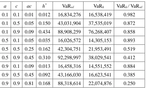
of Heligman-Pollard law are summarized in Tables 1-3. Table 1A shows that the hedging

benefits (as measures of σh / σwl and ) of life settlements to insurance are material in almost all times and can be rather significant. The standard deviation would be reduced by about

10% even when one of the common factor loadings is as low as 0.1. When both life

settlements and insurance have medium loadings of 0.5 with regard to the mortality common

factor, the standard deviation is reduced by almost 50%. The hedging benefits are

immaterial only when the correlation coefficient between the life settlement and insurance

contract is as low as 0.01. The observations that the mortality rates in many countries

exhibit downward trends imply that the loadings would not be small. Our simulation results

therefore indicate that life settlements will render significant hedging benefits to life insurers.

[Insert Table 1A Here]

From Table 1A, We further observe that both measures of the hedging effect, σh / σwl and , increase with a and c, respectively. The hedge ratio increases with these two loadings as well. The risk of the insurance portfolio (σwl) also rises significantly with both loadings, which further demonstrates the hedging benefits of life settlements. For instance, σwl rises from $9,285,807 to $23,222,054 when c is 0.5 instead of 0.1 holding a as 0.5, and life

settlements can reduce the mortality risk to $12,488,106. The above results imply that the

hedging benefits are there when the insurer needs them.

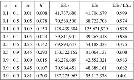
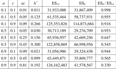
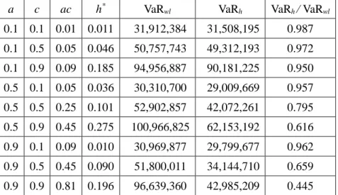
Comparing Tables 1B and 1C with Table 1A, we see that the hedging benefits of life

settlements to insurance remain intact, if they are not more significant, when we change the

risk measure from standard deviation to VaR and expected shortfall. The extent of the risk

reduction is even larger when we adopt VaR or expected shortfall rather than standard

deviation σ. For instance, the risk of the hedged portfolio is 51.9% and 48.6% of the un-hedged portfolio in terms of VaR and expected shortfall, respectively, given that both a and c

are 0.5. The ratio in terms of standard deviation σ in Tables 1A is 53.8%. The results of Tables 1B and 1C support that life settlements seem to provide more hedging benefits for

downside risks than for the deviation risk.

[Insert Tables 1B and 1C Here]

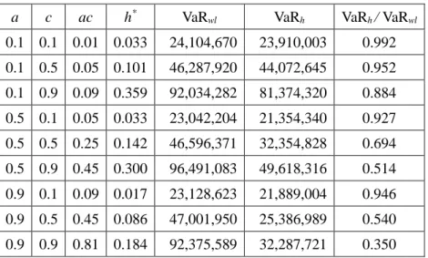
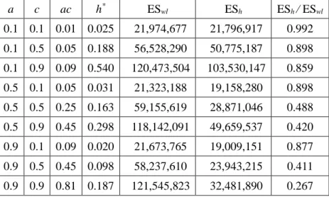
The set of Tables 2 and 3 summarize the hedging effects of life settlements by fitting

mortality rates with the Heligman-Pollard law but with different values of b and d, the risk

loadings specific to life settlement and in the insurance portfolio, respectively. In

comparing of Table 2 with that of Table 1, we notice that the hedging benefits of life

settlements decrease with b and d. For instance, VaRh / VaRwl increases from 0.519 to 0.694 when b and d increase from 0.02 to 0.03, given that a and c are 0.5. The reduction in

hedging benefits is reasonable due to the increase in the specific risk factor relative to the

common factor. The numbers in the set of Table 3 further confirms the above findings and

speculations.

[Insert the sets of Table 2 and 3 here]

The sets of Tables 1-3 result from fitting mortality rates with the Heligman-Pollard law

while the sets of Tables 4-6 are obtained by scaling the mortality rates of the SSA table. All

the above observations support that our results are robust across mortality rate models.

The results of Tables 1-3 are very similar to those of Tables 4-6. For example, using life

settlements can reduce the expected shortfall by more than 50% given that a and c are 0.5 as

we can see from Table 4C. The results also demonstrate that the hedging benefits rendered

by life settlements are similar under alternative mortality rate models.

[Insert the sets of Tables 4 to 6 here]

4. Conclusions and Future Works

This article investigates the hedging potential of the life settlements to life insurance

companies. This paper adds a new contribution to the insurance literature by conducting the

first analysis of life settlements as a hedging vehicle and measuring the hedging benefits for

life insurers. We calibrate our mortality rate models using the real-case data provided by

Coventry and consider the variations in the deviations from life expectancy within and

between life settlements and insurance products. We then propose a hedging approach to

calculate the optimal investment amount for life settlements so that the mortality risk of a life

insurance portfolio can be minimized. The hedging benefits rendered by life settlements are

also quantified under various settings of correlation structures with respect to different risk

measurements including standard deviation, value at risk and expected shortfall. The results

from our numerical examples demonstrate that the proposed hedging strategy could help life

insurers to effectively mitigate the mortality risk to a meaningful extent in most cases. We

speculate that the hedging benefits would be substantial due to the global trends in mortality

improvements that suggested medium to high loadings of the common factor between life

settlements and insurance products even across countries. Our numerical results

demonstrate that adding life settlements to an insurer’s investment asset can reduce the

standard deviation of insurance portfolio by about 10-50% under different settings of

correlation parameters. In addition, the results of risk measurements of value at risk and

expected shortfall support that life settlements provide more hedging benefits for downside

risks than for the deviation risk. The findings of this paper are robust across risk measures,

parameter values, and mortality rate models. Life settlements, therefore, can be used as an

effective hedging vehicle in addition to their good risk-return characteristics as identified in

Braun, Gatzert, and Schmeiser (2011).

We will conduct some more future works to add important insights into the paper. In

the numerical experiments, we will replace the hypothetical life policy portfolio with an

actual portfolio consisting about 500 whole life policies from a major life insurer in Taiwan.

The required investment returns and mortality tables for computing actuarial values of these

life policies are also available from real practices. We believe that using the real data from

an insurer’s liability will enhance the reliability of the hedge effect for our numerical results.

Furthermore, in order to model the dependence structure of the survival times or default

times, we will adopt the Gaussian factor copula model. In survival analysis, a common

assumption is that of conditional independence in a Cox-Process setup. These types of

models correspond to the Clayton copula (a special case of Archimedean copula). The

assumptions of these models may affect results considerably. Therefore, we will also test

the hedging effectiveness under one of these models.

Third, we will conduct sensitivity tests on the rate of return as well as the mortality

improvements for the life settlements. In this version, we assume the rate of return for the

life settlement is assumed at 12%, which was suggested by Coventry. However, as indicated

in Braun et al. (2011), the actual realized annual return of life settlement index from Dec.

2003 to June 2010 is only about 4.85%. In addition, it is reasonable to assume that the

mortality improvement trend for the sub-group of life settlements may be considerably

different from that for the general insurance policyholder pool since settlement companies

usually target senior policyholders with below average life expectancies,. Therefore, we

will test additional assumptions on loading factors (b and d) for mortality improvements in

the life settlement pool and insurance contract pool, to account for the impacts of this

heterogeneity.

References:

1. Asmussen, S., and Glynn, P. W., 2007, Stochastic Simulation. Algorithms and Analysis. Springer Verlag.

2. Bahna-Nolan, Mary and Chuck Ritzke, 2008 Valuation Basic Table (VBT) Report, SOA.

http://www.soa.org/research/experience-study/ind-life/valuation/2008-vbt-report-tables.aspx

3. Benjamin, B., and Soliman., A. S. (eds.), 1993, Mortality on the Move, Oxford: Institute of Actuaries.

4. Biffis, E., 2005, 'Affine Processes for Dynamic Mortality and Actuarial Valuations,' Insurance: Mathematics and Economics, 37, 443-468.

5. Blake, D. and W. Burrows, 2001, Survivor Bonds: Helping to Hedge Mortality Risk, Journal of Risk and Insurance, 68 (2), 339-348.

6. Blake, D., A. J. G. Cairns, and K. Dowd, 2006a, Living with Mortality: Longevity Bonds and Other Mortality-Linked Securities, British Actuarial Journal, 12, 153-197. 7. Blake, D., A. J. G. Cairns, K. Dowd, and R. MacMinn, 2006b, Longevity Bonds:

Financial Engineering, Valuation, and Hedging. Journal of Risk and Insurance, 73 (4), 647-672.

8. Braun, A., N. Gatzert, and H. Schmeiser, 2011, Performance and Risks of Open-End Life Settlement Funds, Journal of Risk and Insurance, forthcoming.

9. Brouhns, N., Denuit, M., and Vermunt, J. K., 2002, 'A Poisson Log-Bilinear Regression Approach to the Construction of Projected Life Tables,' Insurance: Mathematics and Economics, 29, 75-108.

10. Burtschell, X., and J. Gregory et al., 2009, A Comparative Analysis of CDO Pricing Models under the Factor Copula Framework. The Journal of Derivatives, 16(4), 9-37. 11. Hull, J. C., 2011, Options, Futures, and Other Derivatives, 8th ed., Prentice Hall. 12. Cairns, A. J. G., D. Blake, and K. Dowd, 2006a, Pricing Death: Frameworks for the

Valuation and Securitization of Mortality Risk, ASTIN Bulletin, 36, 79-120.

13. Cairns, A. J. G., Blake, D., and Dowd, K., 2006b, 'A Two-Factor Model for Stochastic Mortality with Parameter Uncertainty: Theory and Calibration,' Journal of Risk and Insurance, 73, 687-718.

14. Conning & Company, 2007, Conning Research: Annual Life Settlement Volume Rises to $6.1 Billion in 2006. World Wide Web: www.conning.com (accessed October 4, 2010). 15. Cowley, A. and J. D. Cummins, 2005, Securitization of Life Insurance Assets and

Liabilities, Journal of Risk and Insurance, 72, 193-226.

16. Cox, J. C., J. E. Ingersoll, and S. A. Ross, 1985, A Theory of the Term Structure of Interest Rates, Econometrica 53: 385-407.

17. Cox, S. H. and Y. Lin, 2007, Natural Hedging of Life and Annuity Mortality Risks,

North American Actuarial Journal, 11 (3), 1-15.

18. Cox, S. H., Y. Lin, and S.N. Wang, 2006, Multivariate Exponential Tilting and Pricing Implications for Mortality Securitization. Journal of Risk and Insurance, 73, 719-736. 19. Dahl, M., 2004, ' Stochastic Mortality in Life Insurance: Market Reserves and

Mortality-Linked Insurance Contracts,' Insurance: Mathematics and Economics, 35, 113-136. 20. Dahl, M. and T. Miller, 2006, Valuation and Hedging of Life Insurance Liabilities with

Systematic Mortality Risk. Insurance: Mathematics and Economics, 39, 193-217. 21. Dahl, M., M. Melchior, and T. Miller, 2008, On Systematic Mortality Risk and

Risk-minimization with Survivor Swaps. Scandinavian Actuarial Journal, 2(3), 114-146. 22. Deloitte, 2005, The Life Settlements Market, An Actuarial Perspective on Consumer

Economic Value, Research Report with the University of Connecticut.

23. Denuit, M., P. Devolder, and A. C. Goderniaux, 2007, Securitization of Longevity Risk: Pricing Survivor Bonds with Wang Transform in the Lee-Carter Framework. Journal of Risk and Insurance, 74, 87-113.

24. Doherty, N. A., and H. J. Singer, 2002, The Benefits of a Secondary Market for Life Insurance Policies, Working Paper, Wharton Financial Institutions Center.

25. Dowd, K., 2003, 'Survivor Bonds: A Comment on Blake and Burrows,' Journal of Risk and Insurance, 70, 339-348.

26. Dowd, K., D. Blake, A. J. G. Cairns, and P. Dawson, 2006, Survivor Swaps. Journal of Risk and Insurance, 73, 1-17.

27. Embrechts, P., 2009, Copulas: A Personal View, Journal of Risk and Insurance, 76(3): 639-650.

28. Freedman, M., 2007, STOLI: Fact and Fiction—Combating STOLI Without Violating Consumer Rights, California Broker, December.

29. Gatzert, N., G. Hoermann, and H. Schmeiser, 2009, The Impact of the Secondary Market on Life Insurers’ Surrender Profits, Journal of Risk and Insurance, 76(4): 887- 908.

30. Gatzert, N., 2010, The SecondaryMarket for Life Insurance in the U.K., Germany, and the U.S.: Comparison and Overview, Risk Management and Insurance Review, 13(2): 279-301.

31. Gerstner, T., M. Griebel, M. Holtz, R. Goschnick, and M. Haep, 2008, A General Asset-liability Management Model for the Efficient Simulation of Portfolios of Life Insurance Policies, Insurance: Mathematics and Economics, 42, 704-716.

32. Giacalone, J. A., 2001, Analyzing an Emerging Industry: Viatical Transactions and the Secondary Market for Life Insurance Policies, Southern Business Review, 27(1): 1-7. 33. Grundl, H., T. Post., and R. N. Schulze, 2006, To Hedge or Not to Hedge: Managing

Demographic Risk in Life Insurance Companies, The Journal of Risk and Insurance, 73 (1), 19-41.

34. Heligman, L. and J. H. Pollard, 1980, The Age Pattern of Mortality, Journal of the

Institute of Actuaries, 107, 49-80.

35. Ingraham, H. G., and S. S. Salani, 2004, Life Settlements as a Viable Option, Journal of Financial Service Professionals, 58(5): 72-76.

36. Jalen L. and R. Mamon, 2009, Valuation of Contingent Claims with Mortality and Interest Rate Risks, Mathematical and Computer Modelling, 49, 1893-1904.

37. Kamath, S., and T. Sledge, 2005, Life Insurance Long View—Life Settlements Need Not Be Unsettling, Bernstein Research Call, March 4, 2005 (New York: Sanford C.

Bernstein & Co., LLC).

38. Leimberg, S. R., M. D. Weinberg, B. T. Weinberg, and C. J. Callahan, 2008, Life

Settlements: Know When to Hold and Know When to Fold, Journal of Financial Service Professionals, 62(5): 61-72.

39. Lin, Y. and Cox, S.H., 2005, Securitization of Mortality Risks in Life Annuities, Journal of Risk and Insurance, 72, 227-252.

40. Mason, J., and H. J. Singer, 2008,AReal Options Approach to Valuing Life Settlements Transactions, Journal of Financial Transformation, 23: 61-68.

41. Marceau, E. and P. Gaillardetz, 1999, On Life Insurance Reserve in a Stochastic Mortality and Interest Rates Environment, Insurance: Mathematics and Economics 25 (3), 261-80.

42. McDonald, A. S., Cairns, A. J. G., Gwilt, P. L., and Miller, K. A., 1998, 'An International Comparison of Recent Trends in the Population Mortality,' British Actuarial Journal, 3, 3-141.

43. Mileysky, M. A., and Promislow, S. D., 2001, 'Mortality Derivatives and the Option to Annuities,' Insurance: Mathematics and Economics, 29, 299-318.

44. Milliman Inc., 2008, Life Settlement Characteristics and Mortality Experience for Two Providers, Milliman Research Report, April 2008. World Wide Web: www.milliman.com (accessed October 4, 2010).

45. Ortiz, C. E., C. A. Stone, and A. Zissu, 2008, Securitization of Senior Life Settlements: Managing Interest Rate Risk With a Planned Duration Class, Journal of Financial Transformation, 23: 35-41.

46. Pitacco, E, M. Denuit, S. Haberman, and A. Olivieri, 2007, Modelling Longevity Dynamics for Pensions and Annuity Business. Oxford University Press.

47. Perera, N., and B. Reeves, 2006, Risk Mitigation for Life Settlements, Journal of Structured Finance, Summer 2006: 55-60.

48. Renshaw, A. E. and S. Haberman, 2003, Lee-Carter Mortality Forecasting with Age Specific Enhancement, Insurance: Mathematics and Economics, 33, 255-272. 49. Russ, J., 2005, Wie gut sind die Lebenserwartungsgutachten bei US-Policenfonds?

World Wide Web: www.ifa-ulm.de (accessed October 4, 2010).

50. Schrager, D. F., 2006, Affine Stochastic Mortality, Insurance: Mathematics and Economics, 38, 81-97.

51. Seitel, C. L., 2006, Inside the Life Settlement Industry: An Institutional Investor’s Perspective, Journal of Structured Finance 12(12): 38-40.

52. Smith, B. B., and S. L. Washington, 2006, Acquiring Life Insurance Portfolios: Diversifying and Minimizing Risk, Journal of Structured Finance, 12(12): 41-45.

53. Stallard, E., 2006, Demographic Issues in Longevity Risk Analysis, The Journal of Risk and Insurance, 73 (4), 575-609.

54. Stone, C. A. and A. Zissu, 2006, Securitization of Senior Life Settlements: Managing Extension Risk, The Journal of Derivatives, 13(3): 66-72.

55. Stone, C. A., and A. Zissu, 2007, The Return on a Pool of Senior Life Settlements, Journal of Structured Finance, 13(2): 62-69.

56. Stone, C. A. and A. Zissu, 2008, Using Life Duration and Life Extension-Convexity to Value Senior Life Settlement Contracts, The Journal of Alternative Investments, 11, 94-108.

57. Wang, J. L. and H. C. Huang et al., 2010, An Optimal Product Mix for Hedging Longevity Risk in Life Insurance Companies: The Immunization Theory Approach, Journal of Risk and Insurance, 77(2), 473-497.

58. Ziser, B., 2006, Life Settlements Today: A Secret No More, Journal of Structured Finance 7(2): 35-37.

59. Ziser, B., 2007, An Eventful Year in the Life Settlement Industry, Journal of Structured Finance 8(2): 1-4.

60. Zollars, D., S. Grossfeld, and D. Day, 2003, The Art of the Deal—Pricing Life Settlements, Contingencies, January/February: 34-38.