國 立 交 通 大 學
應 用 數 學 系
碩 士 論 文
在 C 型代數結構下之 N 相黎曼空間的
單擺運動之確切理論與數值計算
The Exact Theory and Numerical Computations of
Pendulum Motions on Riemann Surface of
Genus N with Cut-Structure of Type C
研 究 生:范名宏
指導教授:李榮耀 教授
在 C 型代數結構下之 N 相黎曼空間的
單擺運動之確切理論與數值計算
The Exact Theory and Numerical Computations of
Pendulum Motions on Riemann Surface of
Genus N with Cut-Structure of Type C
研 究 生:范名宏
Student: Ming-Hong Fan
指導教授:李榮耀 教授
Advisor: Jong-Eao Lee
國 立 交 通 大 學
應 用 數 學 系
碩 士 論 文
A Thesis
Submitted to Department of Applied Mathematics College of Science
National Chiao Tung University In Partial Fulfillment of the Requirements
for the Degree of Master in
Applied Mathematics June 2013
在 C 型代數結構下之 N 相黎曼空間的
單擺運動之確切理論與數值計算
研 究 生:范名宏
指導教授:李榮耀 教授
國 立 交 通 大 學
應 用 數 學 系
摘要
u′′+ sin u = 0 在數學的歸類中是一個二階常微分方程,同時也是單擺運動的數學模型。 應用大學課程所學到的微積分技術,可以得到 ∫ 1 √ 2(E + cos u)du = ∫ dt, 其中 E 是積分常數,並且 u 是時間 t 的函數。 以大學課程的能力,上述的積分是難以處理的,因為 √2(E + cos u) 不 是單值函數。因此我們先探討此常微分方程的解 u(t) 所處的空間,並且討論 sin u 的非線性逼近在此空間上的運算情形,此空間就是 N 相黎曼空間。 除此之外,我們研究橢圓函數,並應用雅可比橢圓函數來分析理想單擺 運動的數學模型,也就是我們在摘要開始時所提到的微分方程 u′′+ sin u = 0 , 並且確實的求解,以及討論解的週期性及相關性質。The Exact Theory and Numerical Computations of
Pendulum Motions on Riemann Surface of
Genus N with Cut-Structure of Type C
Student: Ming-Hong Fan
Advisor: Jong-Eao Lee
Department of Applied Mathematics
National Chiao Tung University
Abstract
u′′+ sin u = 0
is a second order differential equation, which is a pendulum motion.
In the process of solving the O.D.E., we have the integral form ∫ 1 √ 2(E + cos u)du = ∫ dt
where E is the integration constant (a parameter), and u is a function of time t.
The integration is noway to solve due to that√2(E + cos u) is not a single-valued function. So we study the space where the solution u(t) resides, which is a Riemann Surface of genus N when sin u is replaced by the N -th partial sum of its Taylor series (which is a polynomial). And we study the corresponding O.D.E. under this Riemann Surface with the help of Mathematica computations.
Next, we study the classical elliptic function to solve the exact O.D.E.
誌謝
碩士生涯以及論文能夠順利完成,最感謝的人就是指導教授李榮耀 老師。 跟隨老師的這段時間以來,老師從不強硬指示我們該做什麼,而是告訴我們研 究的方向之後,便讓同一團隊的大家各自發揮;大家在過程中各自對於不同的 問題有所困惑,之後互相討論、互相幫助,其中的心路歷程就是最珍貴的;除 了學業,也感謝老師這些時間裡在生活中的協助。感謝李榮耀 老師給我們這麼 好的經歷,能夠成為老師的指導學生真的是萬分有幸。 感謝王夏聲 老師的教導,引領我重新認識實變數函數;感謝郎正廉 老師、 余啓哲 老師,老師的指導與建議使論文得以更臻完備。由衷感謝各位老師。 生活中好多事情都和身邊的朋友們一起走過,在此也要向你們說聲感謝。 謝謝智龍、奕倫,我們日夜相處,一起說笑、一起度過碩士生活的兩年;謝謝 卓時、建偉、仁益,好多時刻,沒有你們的陪伴我都不知道該怎麼渡過;謝謝 竣富 學長,在一群晚輩當中,總能分享我們所沒有的經驗,並且給我們更成熟 的建議,沒有學長,畢業的道路肯定更加艱辛;謝謝團隊的夥伴,我們一同困 惑、一同成長、一同享受最後的成果。謝謝分析、組合組的所有同學,你們每 一個人都是我在交大的生活點滴裡重要的人。短暫的相處雖不如大學四年來的 長久,但因為碩班的生活型態讓彼此緊密依靠;人生之中能有這樣的摯友以及 回憶,就是在交大除了知識以外,我所擁有最大的寶藏了。 預料之外的三年,是我人生中的禮物。感謝教育所嘉凌 姐、師資培育中心 雅怡 姐、佩萱 姐,能在這一年與你們共事,讓我對於碩士生涯的第三年有了 完全不一樣的體驗,這將成為我永難忘懷的經歷與回憶。 最後要感謝我的父母,當我在外地生活的時候,你們總會不時地打電話關 心我,也讓我在身心俱疲地回到台北的時候,能有個完全放鬆的地方。時而嚴Contents
1 Introduction 1
2 Riemann Surface 4
2.1 Introduction . . . 4
2.1.1 Construct the corresponding Riemann Surface . . . 5
2.1.2 The curve in algebraic and geometric structure . . . 12
2.1.3 The a, b-cycles and its equivalent paths . . . . 12
2.1.4 Conclusion of structure of Riemann Surface . . . 16
2.2 The integrals of 1 f (z) over a, b-cycles for horizontal cuts . . . . 17
2.3 The integrals of 1 f (z) over a, b-cycles for vertical cuts . . . . 26
3 Apply Riemann Surface to Nonlinear Approximation of Sine 41 4 Elliptic Functions 50 4.1 General definitions and properties of elliptic functions . . . 50
4.1.1 Introduction . . . 50
4.1.2 Doubly-periodic functions and elliptic functions . . . 51
4.1.3 Period-parallelograms . . . 51
4.2 Weierstrass elliptic function . . . 52
4.2.1 Definition . . . 52
4.2.2 Properties of ℘(z) . . . . 53
4.2.3 The constants e1, e2, e3 . . . 54
4.2.4 The Weierstrass-zeta function . . . 54
4.2.5 Properties of ζ(z) . . . . 55
4.2.6 The Weierstrass-sigma function . . . 56
4.2.7 Properties of σ(z) . . . . 57
4.3 The Theta-functions . . . 58
4.3.1 Definition . . . 58
4.3.2 The four types of Theta-functions . . . 59
4.3.3 Properties of ϑi(z) . . . . 61
4.4 Jacobian elliptic functions . . . 63
4.4.1 Definition . . . 63
4.4.2 Glaisher’s notation for quotients . . . 64
4.4.3 Some relations among Jacobian elliptic functions . . . 64
4.4.4 Some properties of Jacobian functions . . . 65
4.4.5 Elliptic integrals of the first kind . . . 67
4.4.6 The graphs of Jacobian functions . . . 67
5 Exact Theory of the Simple Pendulum Motion 71 5.1 Introduction of the simple pendulum . . . 71
5.2 Analyze the derivation . . . 72
5.3 Apply Jacobian elliptic function to solve the simple pendulum motion 77 5.4 Periods and phase portraits with different total energy . . . 81
List of Figures
2.1 Complex plane and extended complex plane . . . 6
2.2 Place the cuts open . . . 7
2.3 Construct R0 . . . 7
2.4 n = 2N− 1 or 2N . . . . 8
2.5 n = 2N− 1 . . . . 8
2.6 n = 2N . . . 8
2.7 Placing cuts open in both sheets . . . 9
2.8 Together two sheets . . . 9
2.9 N − 1 holes for n = 2N − 1 . . . 10
2.10 Placing cuts open in both sheets . . . 10
2.11 Together two sheets . . . 11
2.12 N − 1 holes for n = 2N . . . 11
2.13 a, b-cycles on complex plane . . . . 13
2.14 a, b-cycles on Riemann Surface . . . . 13
2.15 Homotopic . . . 14
2.16 Cut plane and a, b-cycle of f (z) =√z(z− 1)(z − 2)(z − 3) . . . . 14
2.17 Equivalent paths of a, b-cycle . . . . 15
2.18 a-cycles for 2N − 1 points . . . 19
2.20 a∗-cycles for 2N − 1 points . . . 20
2.21 a∗-cycles for 2N points . . . . 20
2.22 b-cycles for 2N − 1 points . . . 22
2.23 b-cycles for 2N points . . . . 22
2.24 b∗-cycles for 2N − 1 points . . . 23
2.25 b∗-cycles for 2N points . . . . 23
2.26 a-cycles and their equivalent paths a∗ . . . 28
2.27 bj and b∗j of 2N − 1 and 2N points . . . 30
2.28 The areas with 2N − 1 and 2N points in vertical cuts . . . 33
2.29 a, b-cycles in other kind of vertical cuts . . . . 35
2.30 a∗j-cycles in other kind of vertical cuts . . . 36
2.31 b∗j-cycles in other kind of vertical cuts . . . 38
3.1 Branch points and branch cuts . . . 43
3.2 a-cycles . . . . 44 3.3 Equivalent a1-cycle . . . 44 3.4 Equivalent a2-cycle . . . 45 3.5 Equivalent a3-cycle . . . 45 3.6 Equivalent a4-cycle . . . 46 3.7 b-cycles . . . 47 3.8 Equivalent b1-cycle . . . 47 3.9 Equivalent b2-cycle . . . 48 3.10 Equivalent b3-cycle . . . 48 3.11 Equivalent b4-cycle . . . 49 4.1 sn(u,1 2) . . . 68 4.2 sn(u,7) . . . 68
4.3 sn(u, 1) . . . . 68 4.4 cn(u,1 2) . . . 69 4.5 cn(u,7 8) . . . 69 4.6 cn(u, 1) . . . . 69 4.7 dn(u,1 2) . . . 70 4.8 dn(u,7 8) . . . 70 4.9 dn(u, 1) . . . . 70 5.1 Simple pendulum . . . 72
5.2 Analysis via Newton’s second law . . . 73
5.3 Analysis via conservation of energy . . . 74
5.4 Solution curves with E =−1 2, E = 0, and E = 1 2 . . . 82
5.5 Potential energy and phase portrait with E = 0 . . . . 83
5.6 Solution curve with E = 1 . . . . 84
5.7 Potential energy and phase portrait with E = 1 . . . . 84
5.8 Solution curves with E = 3 2, E = 2, and E = 5 2 . . . 85
5.9 Potential energy and phase portrait with E = 3 2 . . . 85
List of Tables
4.1 Summary about sn(u), cn(u) and dn(u) . . . . 67 5.1 Summary about the simple pendulum motion within different E . 87
Chapter 1
Introduction
In this paper, we want to study a pendulum motion. An ideal pendulum motion is energy-conservative, and it can be shown in mathematical model as
u′′+ sin u = 0.
Since the ideal pendulum motion is a second order differential equation, [1] we reduce it to a first order differential equation and try to solve it naturally. There is u′u′′+ u′sin u = 0, and 1 2(u ′)2− cos u = E
where E is the integration constant, then
u′ = du
dt =±
√
2(E + cos u) where u is a function of time t,
∫ 1 √ 2(E + cos u)du = ∫ dt. (1.1)
Although we together all skills of integration in calculus, we still has no ability to deal with the equation (1.1). So we change the point to discuss where the solution u(t) resides in short term.
Let f (z) = √2(E + cos u). Since the f (z) is in the type of radical ex-pression, the output of f (z) needs to be confirmed in some domain. For any
E + cos u ∈ C, it can be shown in the polar form, E + cos u = z = |z|eiθ, and, f (z) is a two-valued function of z on complex plane C since |z|eiθ = |z|eiθ+2nπ.
Indeed, f (z) works on Riemann Surface, [2] [3] and the computations of the in-tegral on Riemann Surface rely on the theorems of complex analysis, mainly the Cauchy integral formula. [4]
After studying the Riemann Surface, we use the tools of computing by Mathematica [5] on Riemann Surface applying to the nonlinear approximation of sin u into PN(u) = u−
u3 3! + u5 5! − u7 7! + u9
9! by the Taylor expansion, sin u =
∞ ∑ n=0 (−1)n (2n + 1)!x 2n+1.
Since we are trapped into the equation (1.1), i.e., we are not able to inte-grate the fraction √ 1
2(E + cos u), trying a brand-new theory is the idea to know the exact theorem of the pendulum motion.
By the equation (1.1), we transferred the nonlinear O.D.E. problem into the so-called inverse problem (in an integral form), and it can be replaced by elliptic functions. [6] Furthermore, solve and express the solutions u(t) in terms
of classical elliptic functions. [7]
To construct the theorem enough to solve the original question, the pen-dulum motion, we will introduce several cases of elliptic functions, including the definitions, properties, and relations among each other.
Consider the condition in ideal environment, the pendulum motion works without friction, we can derive the mathematical model of the simple pendulum motion.
In addition, discuss the reasonable E as the total energy in the sense of physics and take the place of equation (1.1) by Jacobian elliptic functions so that it yields the exact solutions and the periods case by case.
Chapter 2
Riemann Surface
2.1 Introduction
u′′+ PN(u) = 0 is also a second order different equation where the degree
of polynomial PN(u) is N .
By the derivation, we have ∫ 1 √ 2(E− PN +1(u))du = ∫ dt
where E is the integration constant.
According to the fundamental theorem of Algebra, there is √ 2(E− PN +1(u)) = v u u tcN +1∏ k=1 (u− uk), c∈ C,
Actually, f (z) = v u u t∏n k=1
(z− zk) is a two-valued function of z on complex plane C. We use algebra and analysis to develop a new surface such that f be-comes a single-valued and analytic function on this surface, namely, a Riemann Surface. [2]
2.1.1 Construct the corresponding Riemann Surface
First, take f (z) = √z for example, f : C → C. Using polar form, let
z =|z|eiθ =|z|ei(θ+2nπ), n∈ Z, then
f (z) =√z =|z|12e θ+2nπ 2 i = |z|1 2e θ 2i if n is even −|z|1 2e θ 2i if n is odd
is a two-valued function. Now we want to let f (z) becomes a single-valued func-tion, so we modify its domainC to develop the corresponding Riemann Surface such that f becomes a single-valued and analytic function on this surface.
Starting at z = reiθ, we have f (z) = √z = √reθ2i, r ̸= 0. Fixing r and
continuing along a closed path once around the origin so that θ increase by 2π, f (z) comes to the value√reθ+2π2 i =−√re
θ
2i which is just the negative of its
original value. Continuing above way then θ increase by 2π and f (z) comes to original value. First, image two sheets lying over the complex plane and cut the plane along negative real axis (i.e. from zero to infinite) and restrict ourselves so as never to continue f (z) over this cuts, we get single-valued branches of f (z).
Define that f (z) =|z|12e iθ 2, −π ≤ θ < π, f (z) =|z|12e iθ 2, π≤ θ < 3π,
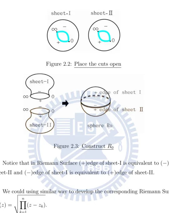
called sheet-I and sheet-II respectively. The cut in each sheet has two edges, label the edge of starting edge with + and the edge of terminal edge with − (Show in Figure 2.1). Moreover, we cross the cut and pass from one sheet to another. Second we extend the plane of complex numbers with one additional point at infinity constitute a number system known as the extended complex numbers. Use stereographic projection, we can consider the two sheets to be a sphere.
Figure 2.1: Complex plane and extended complex plane
Next, image that the spheres are made of rubber and stretch each cut into circular holes.
Rotate the spheres until the holes face each other, and paste two cuts to-gether (+)edge of sheet-I with (−)edge of sheet-II and (−)edge of sheet-I with (+)edge of sheet-II. We can derive a sphere. We called this sphere, Riemann Surface of genus 0, denoted R0. Show in Figure 2.3.
Figure 2.2: Place the cuts open
Figure 2.3: Construct R0
Notice that in Riemann Surface (+)edge of sheet-I is equivalent to (−)edge of sheet-II and (−)edge of sheet-I is equivalent to (+)edge of sheet-II.
We could using similar way to develop the corresponding Riemann Surface for f (z) = v u u t∏n k=1 (z− zk).
In general situation, using same idea to construct Riemann Surface of f (z) where f (z) = v u u t∏n k=1 (z− zk) = n ∏ k=1 √ (z− zk), zk ∈ R, z1 > z2 > . . . > zn for
horizontal cuts. First, we cut plane starts from zk to−∞. If the curve cross even
has a branch cut.
Figure 2.4: n = 2N − 1 or 2N
Case 1: If n = 2N−1. There are cuts along (−∞, z2N−1], . . . , [z2j, z2j−1], . . . , [z4, z3], [z2, z1].
Figure 2.5: n = 2N − 1
Case 2: If n = 2N . There are cuts along [z2N, z2N−1], . . . , [z2j, z2j−1], . . . , [z4, z3], [z2, z1].
We use same idea to construct the corresponding Riemann Surface:
Case 1: n = 2N− 1
Figure 2.7: Placing cuts open in both sheets
Figure 2.9: N − 1 holes for n = 2N − 1
It becomes Riemann Surface with N − 1 holes, that is RN−1.
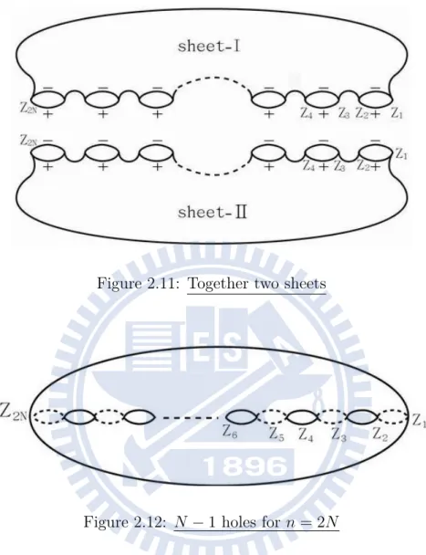
Case 2: n = 2N
Figure 2.11: Together two sheets
Figure 2.12: N − 1 holes for n = 2N
It also becomes Riemann Surface with N − 1 holes, that is RN−1.
So f (z) = v u u t2N∏−1 k=1 (z− zk)or= v u u t∏2N k=1 (z− zk)
will make N cuts and construct Riemann Surface of genus N−1, i.e., N −1 holes in its geometric graph.
2.1.2 The curve in algebraic and geometric structure
For convenience, we use algebraic to discuss and compute the integrals later. We already know the relation of algebraic and geometric structure with
f (z) = v u u t∏n k=1
(z− zk) and how to create the Riemann Surface.
We defined something as follow:
1. The curve in sheet-I is solid line and the curve in sheet-II is dash line in
algebraic structure.
2. The curve in overhead Riemann Surface is solid line and the curve in ventral
Riemann Surface is dash line in geometric structure.
2.1.3 The a, b-cycles and its equivalent paths
We know every closed curve on Riemann Surface RN can be deformed into
an integral combination of the loop-cut ai and bi, i = 1, 2, . . . , N . So in this
paper, we will consider the integrals of f (z) over a, b-cycles help us to obtain the integrals easier.
Figure 2.13: a, b-cycles on complex plane
Figure 2.14: a, b-cycles on Riemann Surface
Each a-cycles are non-overlapping and each b-cycles are non-overlapping. Also a, b-cycles have the same number.
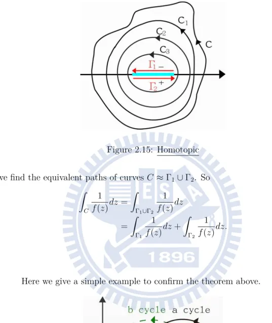
Sometimes the curves are difficult to write out their parameters, but always easy to straight lines. It could help us quicker and easier to obtain the integrals over the curves. So now using homotopic of curves to find the equivalent paths of curves. Take an example to explain.
From C is homotopic to C1, denotes C ≈ C1. We have
∫ C 1 f (z)dz = ∫ C1 1 f (z)dz
Figure 2.15: Homotopic we find the equivalent paths of curves C ≈ Γ1 ∪ Γ2. So
∫ C 1 f (z)dz = ∫ Γ1∪Γ2 1 f (z)dz (2.1) = ∫ Γ1 1 f (z)dz + ∫ Γ2 1 f (z)dz. (2.2)
Here we give a simple example to confirm the theorem above.
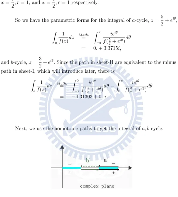
Let f (z) = √z(z− 1)(z − 2)(z − 3) = √z√z− 1√z− 2√z− 3 and a,
b-cycle show as Figure 2.16, then there are two circular paths display the a, b-b-cycle,
x = 5
2, r = 1, and x = 3
2, r = 1 respectively.
So we have the parametric forms for the integral of a-cycle, z = 5 2 + e iθ, ∫ a 1 f (z)dz M ath. = ∫ π −π ieiθ f (52 + eiθ)dθ = 0. + 3.3715i, and b-cycle, z = 3 2+ e iθ
. Sincethe path in sheet-II are equivalent to the minus of path in sheet-I, which will introduce later, there is
∫ b 1 f (z)dz M ath. = ∫ 0 −π ieiθ f (32 + eiθ)dθ− ∫ π 0 ieiθ f (32 + eiθ)dθ = −4.31303 + 0. i.
Next, we use the homotopic paths to get the integral of a, b-cycle.
The equivalent path of a-cycle, from 2 to 3 on the (+)edge in sheet-I and from 3 to 2 on the (−)edge in sheet-I, is called a∗-cycle.
∫ a∗ 1 f (z)dz M ath. = 2 ∫ 2 3 1 f (z)dz = 0. + 3.3715i
The equivalent path of b-cycle, from 1 to 2 in sheet-I and from 2 to 1 in sheet-II, is called b∗-cycle. Similarly, since the path in sheet-II are equivalent to the minus of path in sheet-I, there is
∫ b∗ 1 f (z)dz M ath. = 2 ∫ 2 1 1 f (z)dz = −4.31303 + 0. i
By the calculations above, we verify the theorem for the equivalent path, i.e., homotopic. It means that we can choose the simplest path for the close contour, and get the numerical result in a efficient way.
In the next pages, we will use the skill (2.1) and (2.2) to compute all cases.
2.1.4 Conclusion of structure of Riemann Surface
For arbitrary cut, if f (z) has 2N − 1 or 2N roots, then
1. There are N cuts in complex plane.
2. Its geometric graph has N − 1 holes, and construct corresponding Riemann
Surface of genus N − 1, i.e., RN−1.
2.2 The integrals of
1
f (z)
over a, b-cycles for
hor-izontal cuts
We will use Mathematica helping us to obtain the values of integrals of 1
f (z)
over a, b-cycles. First, discuss the values in sheet-I, sheet-II and Mathematica for horizontal cuts. f (z) = v u u t∏n k=1
(z− zk), using polar form
n
∏
k=1
(z− zk). Let θ1
denotes θ in sheet-I and θ2 denotes in sheet-II. So
θ2 = θ1+ 2π. We have f (z)|(II) = √ reθ22i =√reθ1+2π2 i =√reθ12ieπi =−√reθ12 i =−f(z)| (I)
where f (z)|(I) denote the value of f (z) with z in sheet-I and f (z)|(II) means z
in II. Because the difference of argument between z in I and sheet-II is 2π, there is the difference between f (z)|(I) and f (z)|(II) is π. So, there is
f (z)|(II)=−f(z)|(I).
Now discuss the difference in sheet-I of theory and Mathematica. First,
√
−1 = −i, but we compute √−1 in Mathematica obtain √−1 M ath.
= i. Why?
We found that θ ∈ (−π, π] of reiθ in Mathematica, actually. For any other θ
of reiθ which does not belong to (−π, π], Mathematica will conversion reiθ into reiθ∗, θ∗ ∈ (−π, π] where reiθ = reiθ∗.
Compare the value of f (z) with z in sheet-I and in Mathematica, we dis-cover that Lemma 2.1. If n ∏ k=1
(z− zk) = reiθ in sheet-I for horizontal cut,
f (z)|(I) = f (z)|M athematica if θ ∈ (−π, π), −f(z)|M athematica if θ =−π. Proof.
Since −π does not in (−π, π], Mathematica will conversion re−iπ into reiπ, but f (re−iπ) and f (reiπ) are different.
In theory: − 1 = e−iπ ⇒√−1 = e−iπ2 =−i
In Mathematica: − 1 = e−iπ Math.= eiπ ⇒√−1 = eiπ2 = i
So f (z)M ath.= −f(z) if θ = −π in Mathematica.
In whole paper, f (z) M ath.= −f(z) denotes the polynomial f(z) in front of
M ath.
= is the value of f (z) in theory and the polynomial f (z) behind the M ath.= is the value of f (z) in Mathematica.
Clearly, there is a mistake when θ = −π. When we use Mathematica to get the value of integration we want, we need modify some range where the value will wrong. Determine the difference of sign(f ) (same or negative) and then modify the computation of Mathematica to get right value. Because sometimes the form of integration is complex, if we could simplify the way about modify the difference of sign(f ), it will help us to get right value easier.
Discuss in general situation: Compute
∫ 1
f (z)dz over a, b-cycles for horizontal cuts where f (z) =
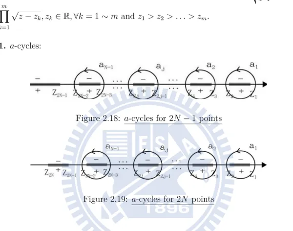
v u u t∏m k=1 (z− zk) = m ∏ k=1 √ z− zk, zk ∈ R, ∀k = 1 ∼ m and z1 > z2 > . . . > zm. 1. a-cycles:
Figure 2.18: a-cycles for 2N − 1 points
Figure 2.19: a-cycles for 2N points
There are N cuts (N− 1 holes), we give that aj is a cycle, center at x with radius r, enclosed [z2j, z2j−1] and doesn’t intersect with other cuts. (parametric
form)
If z ∈ aj, let z = x + reiθ where θ∈ [−π, π),
∫ aj 1 f (z)dz = ∫ aj 1 √∏m k=1(z− zk) dz = ∫ π −π rieiθ ∏m k=1 √ x + reiθ − zkdθ.
2. Consider ∫ a∗j 1 f (z)dz where a ∗
j is an equivalent path for aj and it’s from z2j to
z2j−1 on (+)edge and then from z2j−1 to z2j on (−)edge:
Figure 2.20: a∗-cycles for 2N − 1 points
Figure 2.21: a∗-cycles for 2N points
By Cauchy integral formula, [4] we can get that ∫ aj 1 f (z)dz = ∫ a∗j 1 f (z)dz.
Using Lemma 2.1 to compute:
(i) z2j +
→ z2j−1:
arg(z− zk) = 0 ⇒√z− zkM ath.= √z− zk, k = 2j, 2j + 1, . . . , m arg(z− zk) = −π ⇒√z− zkM ath.= −√z− zk, k = 1, 2, . . . , 2j− 1
So f (z) M ath.= (−1)2j−1f (z) = −f(z), ∫ z2j→z+ 2j−1 1 f (z)dz M ath. = − ∫ z2j−1 z2j 1 f (z)dz. (2.3) (ii) z2j ← z− 2j−1: arg(z− zk) = 0 ⇒√z− zkM ath.= √z− zk, k = 2j, 2j + 1, . . . , m arg(z− zk) = π ⇒√z− zkM ath.= √z− zk, k = 1, 2, . . . , 2j− 1 So f (z) M ath.= f (z), ∫ z2j←z− 2j−1 1 f (z)dz M ath. = ∫ z2j z2j−1 1 f (z)dz. (2.4)
Conclusion of a-cycles: By (2.3) and (2.4), ∫ a∗j 1 f (z)dz M ath. = 2 ∫ z2j z2j−1 1 f (z)dz.
3. b-cycles:
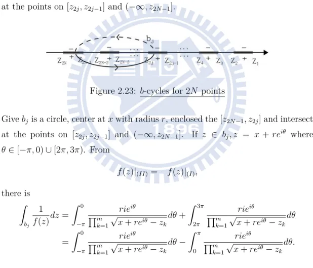
Figure 2.22: b-cycles for 2N− 1 points
Give bj is a circle, center at x with radius r, enclosed the [z2N−1, z2j] and intersect
at the points on [z2j, z2j−1] and (−∞, z2N−1].
Figure 2.23: b-cycles for 2N points
Give bj is a circle, center at x with radius r, enclosed the [z2N−1, z2j] and intersect
at the points on [z2j, z2j−1] and (−∞, z2N−1]. If z ∈ bj, z = x + reiθ where
θ∈ [−π, 0) ∪ [2π, 3π). From f (z)|(II) =−f(z)|(I), there is ∫ bj 1 f (z)dz = ∫ 0 −π rieiθ ∏m k=1 √ x + reiθ− zkdθ + ∫ 3π 2π rieiθ ∏m k=1 √ x + reiθ− zkdθ = ∫ 0 −π rieiθ ∏m k=1 √ x + reiθ− zkdθ− ∫ π 0 rieiθ ∏m k=1 √ x + reiθ− zkdθ.
4. The equivalent path b∗j:
Figure 2.24: b∗-cycles for 2N − 1 points
Figure 2.25: b∗-cycles for 2N points From Cauchy integral formula, we have
∫ bj 1 f (z) = ∫ b∗j 1 f (z)
where b∗j is a path from zm to z2j in sheet-I and then from z2j to zm in sheet-II.
Similarly, using Lemma 2.1 to compute:
(1) The path on cut, i.e., the path from z2s+2 to z2s+1 on (+)edge of sheet-I and
the path from z2s+1 to z2s+2 on (−)edge of sheet-II, s = j, j + 1, . . . , N − 2.
(i) z2s+2 +
→ z2s+1:
arg(z− zk) = 0 ⇒√z− zk M ath.= √z− zk, k = 2s + 2, 2s + 3, . . . , m arg(z− zk) = −π ⇒√z− zk M ath.= −√z− zk, k = 1, 2, . . . , 2s + 1
So f (z) M ath.= (−1)2s+1f (z) = −f(z), ∫ z2s+2→z+ 2s+1 1 f (z)dz M ath. = − ∫ z2s+1 z2s+2 1 f (z)dz. (2.5)
(ii) z2s+2 .− z2s+1 on (−)edge of sheet-II is same as on (+)edge of sheet-I,
so consider z2s+2 + ← z2s+1: arg(z− zk) = 0 ⇒√z− zk M ath.= √z− zk, k = 2s + 2, 2s + 3, . . . , m arg(z− zk) = −π ⇒√z− zk M ath.= −√z− zk, k = 1, 2, . . . , 2s + 1 So f (z) M ath.= (−1)2s+1f (z) = −f(z), ∫ z2s+2.− z2s+1 1 f (z)dz M ath. = − ∫ z2s+2 z2s+1 1 f (z)dz. (2.6)
(2) Without cuts, i.e., the path from z2s+1 to z2s in sheet-I and the path from z2s
(i) z2s+1 → z2s: arg(z− zk) = 0 ⇒√z− zk M ath.= √z− zk, k = 2s + 1, 2s + 2, . . . , m arg(z− zk) = −π ⇒√z− zk M ath.= −√z− zk, k = 1, 2, . . . , 2s So f (z) M ath.= (−1)2sf (z) = f (z), ∫ z2s+1→z2s 1 f (z)dz M ath. = ∫ z2s z2s+1 1 f (z)dz. (2.7)
(ii) z2s+1 . z2s, by f (z)|(II)=−f(z)|(I), we consider z2s+1 ← z2s first:
arg(z− zk) = 0 ⇒√z− zk M ath.= √z− zk, k = 2s + 1, 2s + 2, . . . , m arg(z− zk) = −π ⇒√z− zk M ath.= −√z− zk, k = 1, 2, . . . , 2s Hence f (z)|z2s+1. z2s = −f(z)|z2s+1←z2s M ath. = −(−1)2sf (z)|z2s+1←z2s = −f(z)|z2s+1←z2s, ∫ z2s+1. z2s 1 f (z)dz M ath. = − ∫ z2s+1 z2s 1 f (z)dz. (2.8)
Conclusion of b-cycles: By (2.5), (2.6), (2.7) and (2.8), ∫ b∗j 1 f (z)dz M ath. = N∑−1 s=j ( 2 ∫ z2s z2s+1 1 f (z)dz ) .
2.3 The integrals of
1
f (z)
over a, b-cycles for
ver-tical cuts
After knowing the integrals in horizontal cuts introducing in the previous section, we will discuss the integrals for vertical cuts. In this case, we define that
z− zk = reiθ, θ∈ [−3π 2 , π 2) if z in sheet-I z− zk = reiθ, θ∈ [π 2, 5π 2 ) if z in sheet-II,
the cut in each sheet has two edges, label the starting edge with + and the terming edge with − and zk is the end point of vertical cut.
As the previous section, we need to modify the computation in Mathemat-ica such that the numerMathemat-ical result of MathematMathemat-ica is identMathemat-ical to the numerMathemat-ical result of theory when θ∈ [−3π
2 ,−π].
Lemma 2.2. When z in sheet-I for vertical cut whose one of the end points is
zk, √ z− zkM ath.= −√z− zk if arg(z− zk)∈ [−3π 2 ,−π], √ π
Proof.
Let z in sheet-I and using polar form z− zk = reiθ. When θ ∈ (−π,π
2), the argu-ment in theory or Mathematica is the same. When θ∈ [−3π
2 ,−π], Mathematica will conversion θ into θ + 2π where θ + 2π∈ [π
2, π] and re
iθ = re(θ+2π)i, but
In theory: √z− zk =√reθ2i In Mathematica: √z− zk =√reθ+2π2 i =−√re θ 2i Thus, if θ∈ [−3π 2 ,−π], √ z− zkM ath.= −√z− zk.
As same as horizontal cut. We first discuss the difference between the value in theory and the value in Mathematica. Compare their sign(f ) is different or not? Using statement before about modify and get value, the result will be the same or not?
Discuss in general situation of case 1: Compute
∫ 1
f (z)dz over a, b-cycles for vertical cuts where f (z) =
v u u t∏m k=1 (z− zk) = m ∏ k=1 √ z− zk, zk = rki, rk ∈ R, ∀k = 1 ∼ m and r1 < r2 < . . . < rm.
1. a-cycles:
Figure 2.26: a-cycles and their equivalent paths a∗
aj is a cycle, center at x with radius r, enclosed [z2j, z2j−1] and doesn’t
intersect with other cuts. ∫ aj 1 f (z)dz = ∫ a∗j 1
f (z)dz in sheet-I. The equivalent
path a∗j is the path on a vertical cut from z2j to z2j−1 on (+)edge and then from
z2j−1 to z2j on (−)edge.
Using Lemma 2.2 to compute:
(i) z2j + → z2j−1: arg(z− zk) = −π 2 ⇒ √ z− zk M ath.= √z− zk, k = 2j, 2j + 1, . . . , m arg(z− zk) = −3π 2 ⇒ √ z− zk M ath.= −√z− zk, k = 1, 2, . . . , 2j− 1
So f (z) M ath.= (−1)2j−1f (z) = −f(z), ∫ z2j + →z2j−1 1 f (z)dz M ath. = − ∫ z2j−1 z2j 1 f (z)dz. (2.9) (ii) z2j ← z− 2j−1: arg(z− zk) =−π 2 ⇒ √ z− zk M ath.= √z− zk, k = 2j, 2j + 1, . . . , m arg(z− zk) =−π 2 ⇒ √ z− zk M ath.= √z− zk, k = 1, 2, . . . , 2j − 1 So f (z) M ath.= f (z), ∫ z2j←z− 2j−1 1 f (z)dz M ath. = ∫ z2j z2j−1 1 f (z)dz. (2.10)
Conclusion of a-cycles of case 1: By (2.9) and (2.10), ∫ a∗j 1 f (z)dz M ath. = 2 ∫ z2j z2j−1 1 f (z)dz. 2. b-cycles:
bj is a cycle, center at x with radius r, enclosed [z2N−1, z2j] and intersect
the points on [z2j, z2j−1] and [z2N−1, z2N] in the case of 2N points, or bj is a
Figure 2.27: bj and b∗j of 2N − 1 and 2N points
[z2j, z2j−1] and [z2N−1,∞) in the case of 2N − 1 points.
By Cauchy integral formula, we know that ∫ bj 1 f (z)dz = ∫ b∗j 1 f (z)dz
where b∗j is a path from zm to z2j in sheet-I and then from z2j to zm in sheet-II.
Similarly, using Lemma 2.2 to compute:
(1) The path on cut, i.e., the path from z2s+2 to z2s+1 on (+)edge of sheet-I and
the path from z2s+1 to z2s+2 on (−)edge of sheet-II, s = j, j + 1, . . . , N − 2.
(i) z2s+2 + → z2s+1: arg(z− zk) = −π 2 ⇒ √ z− zk M ath.= √z− zk, k = 2s + 2, 2s + 3, . . . , m arg(z− zk) = −3π ⇒√z− zk M ath.= −√z− zk, k = 1, 2, . . . , 2s + 1
So f (z) M ath.= (−1)2s+1f (z) = −f(z), ∫ z2s+2→z+ 2s+1 1 f (z)dz M ath. = − ∫ z2s+1 z2s+2 1 f (z)dz. (2.11)
(ii) z2s+2 .− z2s+1 on (−)edge of sheet-II is same as on (+)edge of sheet-I,
so consider z2s+2 + ← z2s+1: arg(z− zk) = −π 2 ⇒ √ z− zk M ath.= √z− zk, k = 2s + 2, 2s + 3, . . . , m arg(z− zk) = −3π 2 ⇒ √ z− zk M ath.= −√z− zk, k = 1, 2, . . . , 2s + 1 So f (z) M ath.= (−1)2s+1f (z) = −f(z), ∫ z2s+2.− z2s+1 1 f (z)dz M ath. = − ∫ z2s+2 z2s+1 1 f (z)dz. (2.12)
(2) Without cuts, i.e., the path from z2s+1 to z2s in sheet-I and the path from z2s
(i) z2s+1 → z2s: arg(z− zk) = −π 2 ⇒ √ z− zk M ath.= √z− zk, k = 2s + 1, 2s + 2, . . . , m arg(z− zk) = −3π 2 ⇒ √ z− zk M ath.= −√z− zk, k = 1, 2, . . . , 2s So f (z) M ath.= (−1)2sf (z) = f (z), ∫ z2s+1→z2s 1 f (z)dz M ath. = ∫ z2s z2s+1 1 f (z)dz. (2.13)
(ii) z2s+1 . z2s, by f (z)|(II)=−f(z)|(I), we consider z2s+1 ← z2s first:
arg(z− zk) = −π 2 ⇒ √ z− zk M ath.= √z− zk, k = 2s + 1, 2s + 2, . . . , m arg(z− zk) = −3π 2 ⇒ √ z− zk M ath.= −√z− zk, k = 1, 2, . . . , 2s Hence f (z)|z2s+1. z2s = −f(z)|z2s+1←z2s M ath. = −(−1)2sf (z)|z2s+1←z2s = −f(z)|z2s+1←z2s, ∫ z2s+1. z2s 1 f (z)dz M ath. = − ∫ z2s+1 z2s 1 f (z)dz. (2.14)
Conclusion of b-cycles of case 1: By (2.11), (2.12), (2.13) and (2.14), ∫ b∗j 1 f (z)dz M ath. = N∑−1 s=j (2 ∫ z2s z2s+1 1 f (z)dz).
When we want to modify the computation of f (z) which has m roots, we needs to consider √z− zk, k = 1, 2, . . . , m. There are m steps of modifying the
computation, and if m is large, it will become troublesome. Here provides a way to reduce the step. We can divided domain R into many areas to discuss the way to modify on vertical cuts.
If f (z) = v u u t∏m k=1 (z− zk) = m ∏ k=1 √
z− zk for vertical cut in general situation:
Figure 2.28: The areas with 2N − 1 and 2N points in vertical cuts
Case 1: zk = aki, ak∈ R, k = 1, 2, . . . , 2N
Case 2: zk = aki, ak∈ R, k = 1, 2, . . . , 2N − 1
1. z∈ (+)edge of the cut [z2j−1, z2j):
arg(z− zk) =−3π 2 ⇒ √ z− zk M ath.= −√z− zk, k = 1, 2, . . . , 2j− 1 arg(z− zk) =−π 2 ⇒ √ z− zk M ath.= √z− zk, k = 2j, 2j + 1, . . . , 2N− 1 or 2N f (z)M ath.= (−1)2j−1f (z) =−f(z)
2. z∈ (−)edge of the cut [z2j−1, z2j):
arg(z− zk) = π 2 ⇒ √ z− zk M ath.= √z− zk, k = 1, 2, . . . , 2j− 1 arg(z− zk) =−π 2 ⇒ √ z− zk M ath.= √z− zk, k = 2j, 2j + 1, . . . , 2N − 1 or 2N f (z)M ath.= f (z) 3. z∈ {(x, y) : x < 0, a2j−1 ≤ y < a2j} = region-(2j − 1): arg(z− zk)∈ (−3π 2 ,−π] ⇒ √ z− zk M ath.= −√z− zk, k = 1, 2, . . . , 2j− 1 arg(z− zk)∈ (−π, −π 2) ⇒ √ z− zk M ath.= √z− zk, k = 2j, 2j + 1, . . . , 2N − 1 or 2N f (z)M ath.= (−1)2j−1f (z) =−f(z) 4. z∈ {(x, y) : x ≤ 0, a2j ≤ y < a2j+1} = region-(2j): arg(z− zk)∈ [−3π 2 ,−π] ⇒ √ z− zk M ath.= √z− zk, k = 1, 2, . . . , 2j arg(z− zk)∈ (−π, −π 2] ⇒ √ z− zk M ath.= √z− zk, k = 2j + 1, 2j + 2, . . . , 2N − 1 or 2N
5. z∈ {(x, y) : x ≤ 0, y < a1} ∪ {(x, y) : 0 < x}: arg(z− zk)∈ (−π,π 2) ⇒ √ z− zk M ath.= √z− zk, ∀k f (z)M ath.= f (z) Conclusion: f (z)M ath.=
−f(z) if z ∈ region-(2j − 1) ∪ (+)edge of the cut [z2j−1, z2j)
f (z) otherwise
After studying the above skill, now let us discuss the other general case of vertical cuts whose figure showed below by two ways.
Consider f (z) = v u u t∏m k=1 (z− zk) = m ∏ k=1 √ z− zk, where n = 2N, z2k−1 =
z2k, k = 1, 2, . . . , N and Re(z1) > Re(z3) > . . . > Re(z2N−1), also Im(z1) =
Im(z3) = . . . = Im(z2N−1) and Im(z2) = Im(z4) = . . . = Im(z2N).
1. Compute ∫ a∗j 1 f (z)dz where a ∗
j is an equivalent path for aj:
Figure 2.30: a∗j-cycles in other kind of vertical cuts (1) Compute by using argument of complex number to modify:
(i) The path from z2j to z2j−1 on (+)edge of sheet-I:
arg(z− zk)∈ [−3π 2 ,−π] ⇒ √ z− zk M ath.= −√z− zk, k = 1, 3, . . . , 2j − 1 arg(z− zk)∈ (−π,π 2) ⇒ √ z− zk M ath.= √z− zk, k = otherwise f (z)M ath.= (−1)jf (z)
(ii) The path from z2j−1 to z2j on (−)edge of sheet-I:
arg(z− zk)∈ [−3π 2 ,−π] ⇒ √ z− zk M ath.= −√z− zk, k = 1, 3, . . . , 2j − 3 arg(z− zk)∈ (−π,π 2) ⇒ √ z− zk M ath.= √z− zk, k = otherwise f (z)M ath.= (−1)j−1f (z)
By (i), (ii), and Cauchy integral formula, ∫ aj 1 f (z)dz = ∫ a∗j 1 f (z)dz M ath. = (−1)j ∫ z2j−1 z2j 1 f (z)dz + (−1) j−1 ∫ z2j z2j−1 1 f (z)dz = (−1)j2 ∫ z2j−1 z2j 1 f (z)dz.
(2) Using the result about modify of blocks and then we can compute ∫
a∗j
1
f (z)dz:
(i) The path from z2j to z2j−1 on (+)edge of sheet-I:
√ z− z2k−1 √ z− z2k M ath. = −√z− z2k−1 √ z− z2k, k = 1, 2, . . . , j √ z− z2k−1 √ z− z2k M ath. = √z− z2k−1 √ z− z2k, k = j + 1, j + 2, . . . , N f (z)M ath.= (−1)j m ∏ k=1 √ z− zk= (−1)jf (z)
(ii) The path from z2j−1 to z2j on (−)edge of sheet-I:
√ z− z2k−1 √ z− z2k M ath. = −√z− z2k−1 √ z− z2k, k = 1, 2, . . . , j− 1 √ z− z2k−1 √ z− z2k M ath. = √z− z2k−1 √ z− z2k, k = j, j + 1, . . . , N f (z) M ath.= (−1)j−1 m ∏ k=1 √ z− zk= (−1)j−1f (z)
By (i),(ii), we have ∫ aj 1 f (z)dz = ∫ a∗j 1 f (z)dz M ath. = (−1)j ∫ z2j−1 z2j 1 f (z)dz + (−1) j−1 ∫ z2j z2j−1 1 f (z)dz = (−1)j2 ∫ z2j−1 z2j 1 f (z)dz. 2. Compute ∫ b∗j 1 f (z)dz where b ∗
j is an equivalent path for bj, and b∗j =∪Nk=j+1a∗k∪ {z2N → z2j} ∪ {z2N. z2j}:
Figure 2.31: b∗j-cycles in other kind of vertical cuts (1) z ∈ a∗k: done above.
(2) {z2N → z2j} ∪ {z2N. z2j}:
(a) Compute by using argument of complex number to modify:
(i) z2s+2 → z2s (namely b∗s1), s = j, j + 1, . . . , N − 1: arg(z− zk)∈ [−3π 2 ,−π] ⇒ √ z− zk M ath.= −√z− zk, k = 1, 2, . . . , 2s arg(z− zk)∈ (−π,π) ⇒√z− zk M ath.= √z− zk, k = 2s, 2s + 1, . . . , 2N
f (z)M ath.= (−1)2sf (z) = f (z)
(ii) z2s+2. z2s (namely b∗s2), s = j, j + 1, . . . , N − 1. Since f(z)|(II) =
−f(z)|(I), so we consider z2s+2 ← z2s first: arg(z− zk)∈ [−3π 2 ,−π] ⇒ √ z− zk M ath.= −√z− zk, k = 1, 2, . . . , 2s arg(z− zk)∈ (−π,π 2) ⇒ √ z− zk M ath.= √z− zk, k = 2s, 2s + 1, . . . , 2N f (z)M ath.= −(−1)2sf (z) =−f(z)
By (i),(ii), and letting b∗s1∪ b∗s2 = b∗s, we have
∫ b∗s 1 f (z)dz = ∫ b∗s1 1 f (z)dz + ∫ b∗s2 1 f (z)dz M ath. = ∫ z2s z2s+2 1 f (z)dz + (−1) ∫ z2s+2 z2s 1 f (z)dz = 2 ∫ z2s z2s+2 1 f (z)dz.
(b) Using the result about modify of blocks to compute in Mathematica:
(i) z2s+2 → z2s (b∗s1), s = j, j + 1, . . . , N − 1: √ z− z2k−1 √ z− z2k M ath. = √z− z2k−1 √ z− z2k, ∀k f (z) M ath.= f (z)
(ii) z2s+2. z2s (b∗s2), s = j, j + 1, . . . , N − 1. Since f(z)|(II)=−f(z)|(I), so we consider z2s+2 ← z2s first: √ z− z2k−1 √ z− z2k M ath. = √z− z2k−1 √ z− z2k, ∀k f (z) M ath.= −f(z)
By the above compute and Cauchy integral formula, ∫ bj 1 f (z)dz = ∫ b∗j 1 f (z)dz = N ∑ k=j+1 ∫ a∗k 1 f (z)dz + N∑−1 s=j ∫ b∗s 1 f (z)dz M ath. = N ∑ k=j+1 ( (−1)j2 ∫ z2k−1 z2k 1 f (z)dz ) + N−1 ∑ s=j ( 2 ∫ z2s z2s+2 1 f (z)dz ) .
No matter what methods we use, way of areas or the arguments of complex number, the modifying is the same. This means that we could choose the way letting the computation easier for different situation.
Together with the consequences, the next chapter shows how we apply the all conclusions above to a polynomial, surely, we can deal with the computation of known function which we are interesting about its construction on Riemann Surface.
Chapter 3
Apply Riemann Surface to
Nonlinear Approximation of Sine
After the study of previous chapter, we apply the conclusion of Riemann Surface to the approximation of sine, and compute the integration on the Rie-mann Surface. Here we replace sin u by PN(u) = u−u3 3! + u5 5! − u7 7! + u9 9! since sin u = ∞ ∑ n=0 (−1)n (2n + 1)!x
2n+1, the Taylor expansion shows.
So that, there is a new differential equation
u′′+ PN(u) = 0, u′u′′+ u′PN(u) = 0.
Integrating both sides, we obtain 1 2(u
′
where E is the integration constant, PN +1(u) = u2 2! − u4 4! + u6 6! − u8 8! + u10 10!, then u′ = du dt = √ 2(E− PN +1(u)) where u is a function of time t,
∫ 1 √ 2(E− PN +1(u))du = ∫ dt.
According to the fundamental theorem of Algebra, there is √ 2(E− PN +1(u)) = v u u tcN +1∏ k=1 (u− uk), c∈ C.
Let f (u, E) = √2(E− PN +1(u)), here we take E be 1.5, so that we can use Mathematica and obtain
f (u, 1.5) = v u u t∏10 k=1 (u− uk) = 10 ∏ k=1 √ u− uk where u1 =−5.7957 − 3.81789i u2 =−5.7957 + 3.81789i u3 =−5.42043 u4 =−4.26672 u5 =−2.09438 u6 = 2.09438 u7 = 4.26672 u8 = 5.42043 u9 = 5.7957− 3.81789i u10= 5.7957 + 3.81789i.
Hence, we have ten branch points and obtain five branch cuts as the figure below.
Figure 3.1: Branch points and branch cuts
As we learned in Chapter 2, all integration of closed contour on Riemann Surface is homotopic to the linear combination of a, b-cycles since the Cauchy integral formula. Hence, it is going to show the a, b-cycles in the integral
∫ 1 f (u)du = ∫ 1 ∏10 k=1 √ u− ukdu.
Since there exist five branch cuts, there are four a-cycles and four b-cycles we need to discuss, and the following computation will be completed by paramet-ric form. The all closed contour cycles are counterclockwise.
The a-cycles is showed below.
Figure 3.2: a-cycles The equivalent a1-cycle is showed below.
Figure 3.3: Equivalent a1-cycle
∫ a1 1 f (u)du M ath. = 2 ∫ u4 u3 1 f (r)dr = −1.03837 × 10⁻²⁰− 0.00339657i
The equivalent a2-cycle is showed below.
Figure 3.4: Equivalent a2-cycle
∫ a2 1 f (u)du M ath. = 2 ∫ u6 u5 1 f (r)dr = −2.29246 × 10⁻²⁰+ 0.00640376i The equivalent a3-cycle is showed below.
∫ a3 1 f (u)du M ath. = 2 ∫ u8 u7 1 f (r)dr = 2.30733× 10⁻²¹− 0.00339657i The equivalent a4-cycle is showed below.
Figure 3.6: Equivalent a4-cycle
∫ a4 1 f (u)du M ath. = 2 ∫ Im(u10) Im(u9) 1 f (Re(u9) + ri) idr = −3.52366 × 10⁻¹⁹+ 0.000194696i
Hence, we have all numerical results of a-cycles, and the next step is com-puting the b-cycles.
The b-cycles is showed below.
Figure 3.7: b-cycles The equivalent b1-cycle is showed below.
Figure 3.8: Equivalent b1-cycle
∫ b1 1 f (u)du M ath. = 2 ∫ Im(u1) 0 1 f (Re(u1) + ri) idr− 2 ∫ u3 Re(u1) 1 f (r)dr = 0.00226652 + 0.0000973482i
The equivalent b2-cycle is showed below.
Figure 3.9: Equivalent b2-cycle
∫ b2 1 f (u)du M ath. = ∫ b1 1 f (u)du− 2 ∫ u5 u4 1 f (r)dr = −0.00300153 + 0.0000973482i The equivalent b3-cycle is showed below.
∫ b3 1 f (u)du M ath. = ∫ b2 1 f (u)du− 2 ∫ u7 u6 1 f (r)dr = 0.00226652 + 0.0000973482i The equivalent b4-cycle is showed below.
Figure 3.11: Equivalent b4-cycle
∫ b4 1 f (u)du M ath. = ∫ b3 1 f (u)du− 2 ∫ Re(u10) u8 1 f (r)dr + 2 ∫ 0 Im(u10) 1 f (Re(u10) + ri) idr = 8.67362× 10⁻¹⁹− 4.06576 × 10⁻²⁰i
So far, we have all numerical results of a, b-cycles, and, hence, we can obtain any integration of closed contour in this specific case.
Chapter 4
Elliptic Functions
In our original question, we want to solve the different equation
u′′+ sin u = 0,
and since the difficulty in integration, the ideal of solving the equation changes to the theory of elliptic functions. [6] There are several typical cases of elliptic functions, and the following pages will introduce the definitions, properties, and relations among these cases.
4.1 General definitions and properties of elliptic
functions
4.1.1 Introduction
sys-an elliptic function is due to Abel, Jacobi sys-and Gauss. The elliptic function is originated from the problem of finding the circumference of the ellipse, and in the view of differential equations, the elliptic function can solve kinds of problem with complex integrations.
4.1.2 Doubly-periodic functions and elliptic functions
A function f is called periodic with period 2ω if
f (z + 2ω) = f (z).
A function f is called a doubly-periodic function with 2ω1 and 2ω2 if
f (z + 2ω1) = f (z + 2ω2) = f (z)
where 2ω2 2ω1
is not purely real.
Moreover, a doubly-periodic function f is called an elliptic function if it is analytic except poles and has no singularities other than poles in the finite part of the plane.
4.1.3 Period-parallelograms
Suppose that in the plane of the variable z we mark the points 0, 2ω1, 2ω2
and 2ω1+ 2ω2, generally, all the points whose complex coordinates are of the form
2mω1+ 2nω2, where m and n are integers. Consider the points of set 0, 2ω1, 2ω2
ω inside or on the boundary of this parallelogram such that f (z + ω) = f (z)
for all values of z, this parallelogram is called a fundamental period-parallelogram for an elliptic function with periods 2ω1, 2ω2.
Such a translated parallelogram, without zeros or poles on its boundary, is called a cell.
4.1.4 Simple properties of elliptic functions
1. The number of poles of an elliptic function in any cell is finite. 2. The number of zeros of an elliptic function in any cell is finite.
3. The sum of the residues of an elliptic function at its poles in any cell is zero. 4. Liouville’s theorem:
An elliptic function with no poles in a cell is merely a constant.
4.2 Weierstrass elliptic function
4.2.1 Definition
The Weierstrass elliptic function ℘(z) is one of the famous elliptic function, which is defined by the equation
℘(z) = 1 z2 + ∑′{ 1 (z− 2mω − 2nω )2 − 1 (2mω + 2nω )2 } (4.1)
where∑′ denotes that the sum excludes the term when m = n = 0 and ω1, ω2
satisfy the condition that the ratio is not purely real. For brevity, we write Ωm,n
in place of 2mω1+ 2nω2. So that the equation (4.1) will be
℘(z) = 1 z2 + ∑ m,n ′ { (z− Ωm,n)−2− Ω−2m,n } .
4.2.2 Properties of ℘(z)
1. ℘(z) is an even function with single double pole at Ωm,n for integers m, n.
2. ℘(z) satisfies the differential equation
℘′2(z) = 4℘3(z)− g2℘(z)− g3
where g2 and g3 (called the invariants) are given by the equations
g2 = 60 ∑ m,n ′Ω−4 m,n, g3 = 140 ∑ m,n ′Ω−6 m,n. 3. (Properties of homogeneity) ℘(λz; λω1, λω2) = λ−2℘(z; ω1, ω2), λ̸= 0 ℘(λz; λ−4g2, λ−6g3) = λ−2℘(z; g2, g3), λ̸= 0
where ℘(z; ω1, ω2) denote the function formed with periods 2ω1, 2ω2and ℘(z; g2, g3)
denote the function formed with invariants g2, g3.
4. (Addition-theorem) a. If u + v + w = 0, then ℘(u) ℘′(u) 1 ℘(v) ℘′(v) 1 ℘(w) ℘′(w) 1 = 0.
b. ℘(z + y) = 1 4 { ℘′(z)− ℘′(y) ℘(z)− ℘(y) }2 − ℘(z) − ℘(y). c. ℘(2z) = 1 4 { ℘′′(z) ℘′(z) }2 − 2℘(z)
unless 2z is a period. The result is called the duplication formula.
4.2.3 The constants e
1, e
2, e
3Let ℘(z) be the Weierstrass elliptic function with periods 2ω1, 2ω2. The
value ℘(ω1), ℘(ω2), ℘(ω3) (where ω3 =−ω1−ω2) are all unequal; and, if their value
be e1, e2, e3, respectively, then the roots of the cubic equation 4t3− g2t− g3 = 0
and e1 ̸= e2 ̸= e3. We have e1+ e2+ e3 = 0, e2e3+ e3e1+ e1e2 =− 1 4g2, e1e2e3 = 1 4g3.
4.2.4 The Weierstrass-zeta function
First of all, the Weierstrass-zeta function should not be confused with the Zeta-function of Riemann discussed in Chapter XIII in [6].
The Weierstrass-zeta function ζ(z) is defined by the equation
dζ(z)
dz =−℘(z),
coupled with the condition lim
z→0 { ζ(z)− 1 z } = 0.
Since the series for ℘(z)− 1
z2 converges uniformly throughout any domain
from which the neighbourhoods of the points Ω′m,n are excluded, we can integrate term-by-term and get
ζ(z)− 1 z =− ∫ z 0 { ℘(z)− 1 z2 } dz =−∑ m,n ′∫ z 0 { (z− Ωm,n)−2− Ω−2m,n } dz, and so ζ(z) = 1 z + ∑ m,n ′ { 1 z− Ωm,n + 1 Ωm,n + z Ω2 m,n } .
4.2.5 Properties of ζ(z)
1. ζ(z) is an odd function. It is not a doubly-periodic function, and the residue
of ζ(z) at every pole is 1.
2. If we integrate the equations
℘(z + 2ω1) = ℘(z) and ℘(z + 2ω2) = ℘(z),
ζ(z + 2ω1) = ζ(z) + 2η1
ζ(z + 2ω2) = ζ(z) + 2η2
where 2η1 and 2η2 are the constants introduced by integration; putting z =
−ω1, z = −ω2, respectively, and taking account of the fact that ζ(z) is an odd
function, we have η1 = ζ(ω1), η2 = ζ(ω2). 3. (Properties of homogeneity) ζ(λz; λω1, λω2) = λ−1ζ(z; ω1, ω2), λ̸= 0 4. (Legendre’s relation) η1ω2 − η2ω1 = 1 2πi
4.2.6 The Weierstrass-sigma function
The Weierstrass-sigma function σ(z) is defined by the equation
d
dz log σ(z) = ζ(z)
coupled with the condition lim
z→0 { σ(z) z } = 1.
taking the exponential of each side of the resulting equation, we get σ(z) = z∏ m,n ′ { (1− z Ωm,n )exp( z Ωm,n + z 2 2Ω2 m,n ) } .
4.2.7 Properties of σ(z)
1. The product for σ(z) converges absolutely and uniformly in any bounded
domain of values of z.
2. The function σ(z) is an odd integral function of z with simple zeros at all the
points Ωm,n.
3. If we integrate the equations
ζ(z + 2ω1) = ζ(z) + 2η1 and ζ(z + 2ω2) = ζ(z) + 2η2,
we get
σ(z + 2ω1) = c1e2η1zσ(z)
σ(z + 2ω2) = c1e2η2zσ(z)
where c1 and c2 are the constants of integration; to determine c1, c2, we put
z =−ω1, z = −ω2, respectively, and then
σ(ω1) =−c1e−2η1ω1σ(w1),
σ(ω2) =−c2e−2η2ω2σ(w2).
Consequently,
c1 =−e2η1ω1,
4. (Properties of homogeneity)
σ(λz; λω1, λω2) = λσ(z; ω1, ω2)
4.3 The Theta-functions
4.3.1 Definition
Let τ be a (constant) complex number whose imaginary part is positive; and write q = eπiτ, so that |q| < 1.
Consider the function ϑ(z, q), defined by the series
ϑ(z, q) = ∞ ∑ n=−∞ (−1)nqn2e2niz. It is evident that ϑ(z, q) = 1 + 2 ∞ ∑ n=1 (−1)nqn2cos 2nz, and that ϑ(z + π, q) = ϑ(z, q); further ϑ(z + πτ, q) = ∞ ∑ n=−∞ (−1)nqn2q2ne2niz =−q−1e−2iz ∞ ∑ (−1)n+1q(n+1)2e2(n+1)iz,
and so
ϑ(z + πτ, q) =−q−1e−2izϑ(z, q).
In consequence of these results, ϑ(z, q) is called a quasi doubly-periodic function of z, and accordingly 1 and −q−1e−2iz are called the periodicity factors associated with the periods π and πτ respectively.
4.3.2 The four types of Theta-functions
It is customary to write ϑ4(z, q) in place of ϑ(z, q); the other three types of
Theta-functions are then defined as follows:
The function ϑ3(z, q) is defined by the equation
ϑ3(z, q) = ϑ4(z + 1 2π, q) = 1 + 2 ∞ ∑ n=1 qn2cos 2nz.
Next, ϑ1(z, q) is defined by the equation
ϑ1(z, q) =−ieiz+ 1 4πiτϑ4(z + 1 2πτ, q) =−i ∞ ∑ n=−∞ (−1)nq(n+12) 2 e(2n+1)iz = 2 ∞ ∑ n=0 (−1)nq(n+12) 2 sin (2n + 1)z.
Lastly, ϑ2(z, q) is defined by the equation ϑ2(z, q) = ϑ1(z + 1 2π, q) = 2 ∞ ∑ n=0 q(n+12) 2 cos (2n + 1)z. Summary: ϑ1(z, q) = 2 ∞ ∑ n=0 (−1)nq(n+12) 2 sin (2n + 1)z ϑ2(z, q) = 2 ∞ ∑ n=0 q(n+12)2cos (2n + 1)z ϑ3(z, q) = 1 + 2 ∞ ∑ n=1 qn2cos 2nz ϑ4(z, q) = 1 + 2 ∞ ∑ n=1 (−1)nqn2cos 2nz
For brevity, the parameter q will usually not be specified, so that ϑi(z) will
4.3.3 Properties of ϑ
i(z)
1. ϑ1(z) is an odd function and the other Theta-functions are even functions.
2. The zeros of the Theta-functions:
ϑ1(z) = 0, where z = 0 + mπ + nπτ ϑ2(z) = 0, where z = π 2 + mπ + nπτ ϑ3(z) = 0, where z = π 2 + πτ 2 + mπ + nπτ ϑ4(z) = 0, where z = πτ 2 + mπ + nπτ 3. The identity ϑ4 2(0) + ϑ 4 4 = ϑ 4 3(0).
4. Jacobi’s expressions for the Theta-functions as infinite products:
ϑ1(z) = 2q 1 4 sin z ∞ ∏ n=1 (1− q2n)(1− 2q2ncos 2z + q4n) ϑ2(z) = 2q 1 4 cos z ∞ ∏ n=1 (1− q2n)(1 + 2q2ncos 2z + q4n ) ϑ3(z) = ∞ ∏ n=1 (1− q2n)(1 + 2q2n−1cos 2z + q4n−2) ϑ4(z) = ∞ ∏ n=1 (1− q2n)(1− 2q2n−1cos 2z + q4n−2)
5. The differential equation satisfied by the Theta-functions
∂2ϑ3(z|τ) ∂z2 =− 4 πi ∂ϑ3(z|τ) ∂τ
where we may regard ϑ3(z|τ) as a function of two independent variables z and τ.
6. A relation between Theta-functions of zero argument