應用於正交分頻多工技術為基礎之低複雜度接收端基頻框架同步器

全文

(1)國立交通大學電子工程學系碩. 電子研究所碩士班士. 論. 文. 應用於正交分頻多工技術為基礎之低複雜度接收端基頻框架同步器. Study on Low Complexity Baseband Frame Synchronization for OFDM Applications. 學生：張瑋哲指導教授：李鎮宜教授. 中華民國九十四年七月.

(2) 應用於正交分頻多工技術為基礎之低複雜度接收端基頻框架同步器 Study on Low Complexity Baseband Frame Synchronization for OFDM Applications. 研究生：張瑋哲. Student：Wei-Che Chang. 指導教授：李鎮宜. Advisor：Chen-Yi Lee. 國立交通大學電子工程學系電子研究所碩士班碩士論文. A Thesis Submitted to Institute of Electronics College of Electrical Engineering and Computer Science National Chiao Tung University in Partial Fulfillment of the Requirements for the Degree of Master of Science in Electronics Engineering July 2005 Hsinchu, Taiwan, Republic of China. 中華民國九十四年七月.

(3) 應用於正交分頻多工技術為基礎之低複雜度接收端基頻框架同步器研究生：張瑋哲. 指導教授：李鎮宜教授. 摘要在無線通訊的系統中，高速傳輸以及低功率消耗一向是最為關切的兩個研究主題，尤其在近年來發展的超寬頻技術(UWB)中，在接受端的時域同步化需要超過 500MHz 的頻寬，應用於這樣的高速設計，必需使用平行化架構來作資料處理，同時造成功率消耗的線性成長，使得低功率消成為超寬頻技術發展中最大的挑戰。在本論文中，我們藉由改良的比對濾波器 (matched-filter)與動態門檻(dynamic threshold)提出應用於正交多頻分工技術(OFDM)之超寬頻系統的低複雜度框架同步器。在這個設計中，我們使用可以降低比對濾波器複雜度和減少暫存器存取資料次數的演算法來達到低複雜度與低功率消耗的需求，並保持框架同步器的誤差在可接受的範圍之內。此外在平行架構下，不同於一般的設計用多套暫存器存取多重資料流的資料來和多重的比對濾波器作運算，我們基於暫存器共用的觀念，將比對濾波器的資料重新排列後，來讓多重的比對濾波器能夠同時分享一套暫存器的資料，以減少平行架構中所需要的暫存器數量。根據模擬的結果，在 802.11a 的系統平台，我們提出的設計在 10% PER 下所造成的誤差小於 0.35dB 的 SNR；而在超寬頻技術的系統平台，我們提出的設計在 8% PER 下所造成的誤差則是小於 0.45dB 的 SNR。而在硬體的實現上，我們使用.18μm 製程，和一般使用平行架構達到 528MSample/s 的框架同步器相比，我們的設計不但能處理 528MSample/s 的資料，還可以節省 58%的功率消耗和 65%的硬體面積。 i.

(4) Study on Low Complexity Baseband Frame Synchronization for OFDM Applications Student：Wei-Che Chang. Advisor：Dr. Chen-Yi Lee. Department of Electronics Engineering Institute of Electronics National Chiao Tung University. ABSTRACT In wireless communication, high data rates and low power consumption are the main concerns to improve the transmission speed and extend the IC working time. In recent years, ultra-wideband (UWB) has received much attention as a high speed, low power wireless portable device. It requires over 500MSamples/s throughput in time domain synchronization and can be achieved by parallel architecture, leading high power dissipation increasing in linear. Therefore, low power issue becomes the challenge of UWB baseband design. In this thesis, a low-complexity frame synchronizer combining improved matched-filter and dynamic-threshold design is proposed for OFDM-based UWB system. It provides a methodology to reduce matched-filter complexity and redundant access of register-files with an acceptable performance loss. Based on the register-sharing algorithm, single register-files shares received data for parallel matched-filters are developed to achieve 528MSample/s throughput for the 480Mb/s UWB design. Simulation results show the synchronization loss of the propose design can be limited to 0.35dB SNR for 10% PER in IEEE 802.11a WLAN system and 0.45dB SNR for 8% PER of LDPC-COFDM and MB-OFDM UWB systems. In hardware implementation, the proposed design can save 58% power consumption and 65% area cost from the conventional design in 0.18μm CMOS process. ii.

(5) 誌謝不知不覺，在交大已經過了六年的時光，尤其是這兩年的研究生活，身為 SI2 研究室的一份子，過的相當的充實，也學習到了許多專業的知識和技術。. 我要特別感謝李鎮宜教授親切的指導和建議，實驗室學長們熱誠的提攜和討論研究，和同學們及學弟妹們的互相砥礪與合作，多虧了大家不斷的給予我幫助，我才能化阻力為助力，順利的完成這本論文。在這裡還要特別的謝謝一同研究 UWB system 的軒宇學長，瑞元學長，林宏和婉君，和大家一起團隊合作時的努力和交流，讓我能在這個研究領域不斷的成長和精進。還有菁哲學長和建青學長，當我在硬體實現時遇到了瓶頸時，總是依靠著你們豐富的經驗助我度過難關。和各位在一起的時光，相信是我一生無法忘懷的回憶。. 最後還要感謝我的父母，謝謝你們無微不至的愛護，陪我完成了這兩年的碩士學業。感謝我的姊姊以及好友們，在我心情低落的時候，給我繼續向前衝刺的鼓勵及動力。僅將這篇論文獻給你們，表達我內心最真切的感激。. 瑋哲 94 年 7 月 iii.

(6) Contents ABSTRACT….....……………………………………………….………ii Contents……….………………………………………………………...iv List of Figures……….…………………………………………………vii List of Tables………………...…………………………………………xii CHAPTER 1 Introduction ...…………………………………………1 1.1 MOTIVATION .............................................................................................................................1 1.2 REVIEWS OF THE FRAME SYNCHRONIZER DESIGN ....................................................................2 1.3 INTRODUCTION TO OFDM SYSTEM ..........................................................................................3 1.4 OUTLINE OF THIS THESIS ..........................................................................................................7. CHAPTER 2. System Platform……………………………………...9. 2.1 IEEE 802.11A PHY ..................................................................................................................9 2.1.1. System Platform.................................................................................................9. 2.1.2. Frame Format...................................................................................................12. 2.2 ULTRA-WIDEBAND SYSTEM....................................................................................................13 2.2.1. System Platform...............................................................................................13. 2.2.2. Frame Format...................................................................................................16. 2.3 SIMULATED CHANNEL MODEL ................................................................................................17 2.3.1. Multi-Path Fading Channel..............................................................................18. 2.3.2. AWGN Model ..................................................................................................20. 2.3.3. Carrier Frequency Offset Model ......................................................................20. 2.3.4. Sampling Clock Offset Model .........................................................................21. CHAPTER 3 A Low Complexity Frame Synchronizer for OFDM Application…………………………………………..23 iv.

(7) 3.1 FRAME SYNCHRONIZER DATA FLOW .......................................................................................23 3.1.1. Packet Detection ..............................................................................................24. 3.1.2. FFT Window Detection....................................................................................26. 3.2 PROPOSED ALGORITHM ...........................................................................................................29 3.2.1. Most-Significant Taps Scheme ........................................................................29. 3.2.2. Quantization Approach ....................................................................................32. CHAPTER 4. A Low Complexity and High Throughput Frame Synchronizer for OFDM-Based UWB System.……35. 4.1 MOTIVATION ...........................................................................................................................35 4.2 LDPC-COFDM DESIGN.........................................................................................................36 4.2.1. Frame Synchronizer Flow................................................................................36. 4.2.1. 1 Packet Detection………………………………………......37 4.2.1. 2 FFT Window Detection………………………………………..38 4.2.1. 3 Preamble Timing Detection…………………………………. 39 4.2.2. Proposed Algorithm .........................................................................................40. 4.2.2. 1 Tap-Reduction Scheme...…………………………………40 4.2.2. 2 Register-Sharing Algorithm………………..………………….44 4.2.2. 3 Dynamic Threshold Design……………………………………47 4.3 MULTI-BAND OFDM DESIGN.................................................................................................48 4.3.1. Frame Synchronizer (MB-OFDM)Flow： ......................................................50. 4.3.2. Proposed Algorithm .........................................................................................51. 4.3.2. 1 Training AGC………………………………………………51 4.3.2. 2 Band Detection……………………………………………….54 4.3.2. 3 Other Function Block…………………………………………56. CHAPTER 5. Simulation Result and Performance Analysis.……..58. 5.1 SIMULATION OF IEEE 802.11A SYSTEM ..................................................................................58 5.2 SIMULATION RESULT OF LDPC-COFDM SYSTEM .................................................................69 5.2.1. Frame Error Rate of Tap-Reduction Scheme ...................................................69 v.

(8) 5.2.2. Performance of Dynamic Threshold................................................................73. 5.2.3. System Performance ........................................................................................74. 5.3 SIMULATION RESULT OF MB-OFDM SYSTEM ........................................................................76 5.3.1. Boundary Variation Distribution......................................................................76. 5.3.2. System Performance ........................................................................................88. CHAPTER 6 Hardware Implementation and Measured Result...94 6.1 DESIGN ARCHITECTURE ..........................................................................................................94 6.1.1. Detail Architecture of Tap-Reduction Matched-Filter .....................................97. 6.1.2. Detail Architecture of Shared Auto-Correlator ................................................98. 6.1.3. Address-Based Register-Files ........................................................................100. 6.2 HARDWARE MEASURED RESULT ...........................................................................................101 6.3 OFDM-BASED UWB BASEBAND TRANSCEIVER ..................................................................102. CHAPTER 7 Conclusion and Future Work………………………104 Bibliography…………………………………………………………..106. vi.

(9) List of Figures. FIG. 1.1 SPECTRUM OF SINGLE-CARRIER SYSTEM. ..............................................................................4 FIG. 1.2 SPECTRUM OF CONVENTIONAL MULTI-CARRIER SYSTEM. ......................................................4 FIG. 1.3 SPECTRUM OF OFDM SYSTEM ..............................................................................................4 FIG. 1.4 USE IDFT/DFT FOR OFDM MODULATION/DEMODULATION .................................................5 FIG. 1.5 USE CP AS GI TO PREVENT ISI AND MAINTAIN CIRCULAR CONVOLUTION .............................6 FIG. 1.6 SIMPLIFIED BLOCK DIAGRAM OF OFDM SYSTEM..................................................................7 FIG. 2.1 IEEE 802.11A SYSTEM PLATFORM ......................................................................................10 FIG. 2.2 PPDU FRAME FORMAT OF IEEE 802.11A PHY...................................................................12 FIG. 2.3 PLCP PREAMBLE FORMAT...................................................................................................12 FIG. 2.4 AN EXAMPLE OF MB-OFDM SYSTEM FOR TFC (1、2、3、1、2、3) ..............................14 FIG. 2.5 SYSTEM BLOCK DIAGRAM OF OFDM BASED UWB SYSTEM ...............................................16 FIG. 2.6 FRAME FORMAT OF MB-OFDM UWB SYSTEM ..................................................................16 FIG. 2.7 CHANNEL MODEL DATA FLOW OF SIMULATION PLATFORM ...................................................17 FIG. 2.8 MULTI-PATH INTERFERENCE AND ISI EFFECT ......................................................................18 FIG. 2.9 IEEE 802.11A CHANNEL IMPULSE RESPONSE ......................................................................19 FIG. 2.10 UWB CHANNEL IMPULSE RESPONSE .................................................................................19 vii.

(10) FIG. 2.11 LINEAR PHASE SHIFT CAUSED BY CFO ..............................................................................21 FIG. 2.12 SCO EFFECT IN TIME DOMAIN AND FREQUENCY DOMAIN..................................................22 FIG. 3.1 FRAME SYNCHRONIZER DATA FLOW ....................................................................................23 FIG. 3.2 EXAMPLE OF PACKET DETECTION IN PROPOSED DESIGN ....................................................25 FIG. 3.3 FFT WINDOW DETECTION IN AWGN AND MULTI-PATH CHANNEL .......................................27 FIG. 3.4 FFT WINDOW DETECTION IN AWGN AND MULTI-PATH CHANNEL .......................................29 FIG. 3.5 POWER DISTRIBUTION OF C0~C63 AND S[1]~S[64] .................................................................30 FIG. 3.6 ANALYSIS OF MOST SIGNIFICANT TAP NUMBER VERSUS POWER RATIO .................................31 FIG. 3.7 TAP POWER ANALYSIS OF QUANTIZED APPROACH ................................................................32 FIG. 3.8 FER BETWEEN CONVENTIONAL AND QUANTIZATION APPROACH .........................................33 FIG. 4.1 FRAME SYNCHRONIZER FLOW .............................................................................................37 FIG. 4.2 PACKET DETECTION FLOW ...................................................................................................38 FIG. 4.3 PREAMBLE TIMING DETECT FLOW .......................................................................................40 FIG. 4.4 DATA FLOW OF CONVENTIONAL DESIGN WITH 128 TAPS (W=1) ..........................................42 FIG. 4.5 DATA FLOW OF TAP-REDUCTION SCHEME WITH 32 TAPS (W =4, J =3).................................43 FIG. 4.6 EXAMPLE OF TAP-REDUCTION SCHEME WITH PARALLELISM ................................................44 FIG. 4.7 DATA FLOW EXAMPLE OF THE PROPOSED DESIGN ................................................................45 FIG. 4.8 DATA FLOW OF REGISTER-SHARING ALGORITHM WITH 32 TAPS .........................................47 FIG. 4.9 BASEBAND RECEIVED DATA OF LDPC-COFDM SYSTEM...................................................49 FIG. 4.10 BASEBAND RECEIVED DATA OF MB-OFDM SYSTEM .......................................................50 FIG. 4.11 FRAME SYNCHRONIZER FLOW OF MB-OFDM UWB SYSTEM ...........................................50 viii.

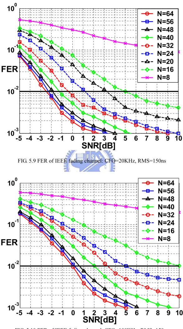
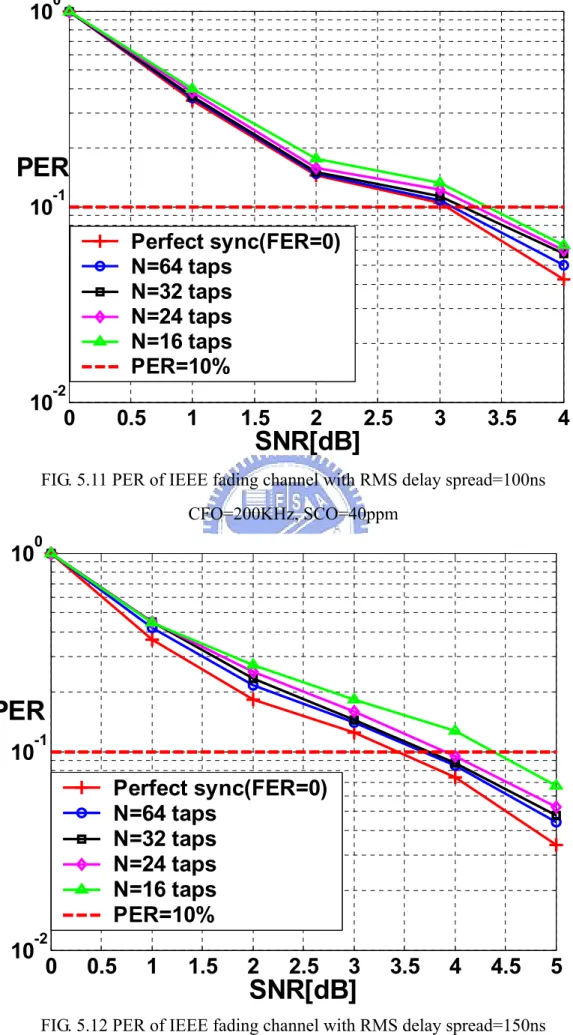
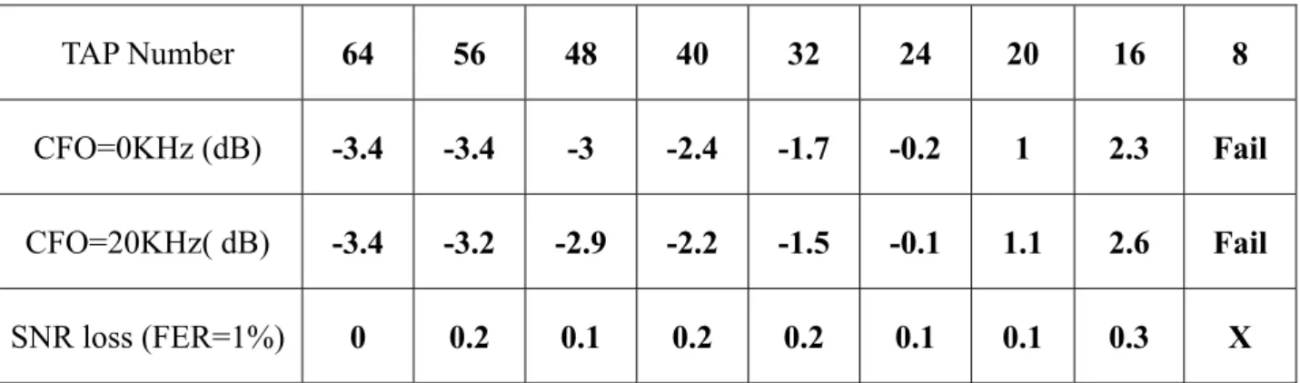
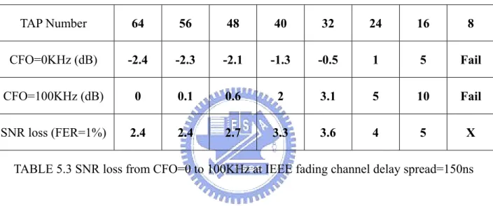
(11) FIG. 4.12 DETAIL DATA FLOW OF TRAINING AGC .............................................................................53 FIG. 4.13 ACCUMULATED POWER OF CONTINUOUS 128 SAMPLES .....................................................54 FIG. 5.1 PER OF PERFECT FRAME SYNCHRONIZATION AT 6MB/S DATA RATE .....................................59 FIG. 5.2 FER OF PURE AWGN CHANNEL, CFO=0KHZ, RMS=0NS .................................................59 FIG. 5.3 FER OF IEEE-FADING CHANNEL: RMS=100NS, CFO=0KHZ ............................................60 FIG. 5.4 FER OF IEEE-FADING CHANNEL: RMS=150NS, CFO=0KHZ ............................................60 FIG. 5.5 FER OF AWGN CHANNEL WITH CFO=20KHZ ...................................................................61 FIG. 5.6 FER OF AWGN CHANNEL WITH CFO=100KHZ .................................................................61 FIG. 5.7 FER OF AWGN CHANNEL WITH CFO=200KHZ .................................................................62 FIG. 5.8 FER OF IEEE-FADING CHANNEL: CFO=20KHZ, RMS=100NS ..........................................62 FIG. 5.9 FER OF IEEE FADING CHANNEL: CFO=20KHZ, RMS=150NS ..........................................63 FIG. 5.10 FER OF IEEE FADING CHANNEL: CFO=100KHZ, RMS=150NS ......................................63 FIG. 5.11 PER OF IEEE FADING CHANNEL WITH RMS DELAY SPREAD=100NS.................................64 FIG. 5.12 PER OF IEEE FADING CHANNEL WITH RMS DELAY SPREAD=150NS ................................64 FIG. 5.13 TAP NUMBER VERSUS FFT WINDOW DETECTION ...............................................................69 FIG. 5.14 TAP-NUMBER VERSUS FRAMER SYNCHRONIZER ................................................................70 FIG. 5.15 TAP-NUMBER VERSUS PER................................................................................................71 FIG. 5.16 SIMULATED THRESHOLD VALUE OF PREAMBLE TIMING DETECTION ...................................72 FIG. 5.17 PERFORMANCE OF DYNAMIC AND FIXED THRESHOLD DESIGN ...........................................72 FIG. 5.18 AWGN CHANNEL, CFO=0KHZ, SCO=0 PPM ..................................................................75 FIG. 5.19 MULTI-PATH CHANNEL RMS DELAY SPREAD=5NS [21], CFO=400KHZ, SCO=40PPM .....75 ix.

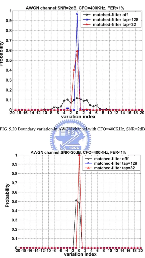
(12) FIG. 5.20 BOUNDARY VARIATION IN AWGN CHANNEL WITH CFO=400KHZ, SNR=2DB ................79 FIG. 5.21 BOUNDARY VARIATION IN AWGN CHANNEL WITH CFO=400KHZ, SNR=20DB ..............79 FIG. 5.22 BOUNDARY VARIATION IN ORIGINAL CM1 CHANNEL, CFO=400KHZ, SNR=2DB............80 FIG. 5.23 BOUNDARY VARIATION IN BEST 90% CM1 CHANNEL, CFO=400KHZ, SNR=2DB ...........80 FIG. 5.24 BOUNDARY VARIATION IN ORIGINAL CM1 CHANNEL, CFO=400KHZ, SNR=20DB..........81 FIG. 5.25 BOUNDARY VARIATION IN BEST 90% CM1 CHANNEL CFO=400KHZ, SNR=20DB ..........81 FIG. 5.26 BOUNDARY VARIATION IN ORIGINAL CM2 CHANNEL, CFO=400KHZ, SNR=2DB............82 FIG. 5.27 BOUNDARY VARIATION IN BEST 90% CM2 CHANNEL, CFO=400KHZ, SNR=2DB ...........82 FIG. 5.28 BOUNDARY VARIATION IN ORIGINAL CM2 CHANNEL, CFO=400KHZ, SNR=20DB..........83 FIG. 5.29 BOUNDARY VARIATION IN BEST 90% CM2 CHANNEL, CFO=400KHZ, SNR=20DB .........83 FIG. 5.30 BOUNDARY VARIATION IN ORIGINAL CM3 CHANNEL, CFO=400KHZ, SNR=2DB............84 FIG. 5.31 BOUNDARY VARIATION IN BEST 90% CM3 CHANNEL, CFO=400KHZ, SNR=2DB ...........84 FIG. 5.32 BOUNDARY VARIATION IN ORIGINAL CM3 CHANNEL, CFO=400KHZ, SNR=20DB..........85 FIG. 5.33 BOUNDARY VARIATION IN BEST 90% CM3 CHANNEL, CFO=400KHZ, SNR=20DB .........85 FIG. 5.34 BOUNDARY VARIATION IN ORIGINAL CM4 CHANNEL, CFO=400KHZ, SNR=2DB............86 FIG. 5.35 BOUNDARY VARIATION IN BEST 90% CM4 CHANNEL, CFO=400KHZ, SNR=2DB ...........86 FIG. 5.36 BOUNDARY VARIATION IN ORIGINAL CM4 CHANNEL, CFO=400KHZ, SNR=20DB..........87 FIG. 5.37 BOUNDARY VARIATION IN BEST 90% CM4 CHANNEL, CFO=400KHZ, SNR=20DB .........87 FIG. 5.38 PER OF CM1 CHANNEL AT DATA RATE=110 MB/S, CFO=400KHZ, SCO=40PPM ............90 FIG. 5.39 PER OF CM2 CHANNEL AT DATA RATE=110 MB/S, CFO=400KHZ, SCO=40PPM ............90 FIG. 5.40 PER OF CM3 CHANNEL AT DATA RATE=110 MB/S, CFO=400KHZ, SCO=40PPM ............91 x.

(13) FIG. 5.41 PER OF CM4 CHANNEL AT DATA RATE=110 MB/S, CFO=400KHZ, SCO=40PPM ............91 FIG. 5.42 PER AT 110~480 MB/S DATA RATE FOR REQUIRED WORST CM CHANNEL .........................92 FIG. 5.43 PER VERSUS TRANSMISSION DISTANCE AT CFO=400KHZ, SCO=40PPM ..........................93 FIG. 6.1 ARCHITECTURE OF PROPOSED FRAME SYNCHRONIZER ........................................................95 FIG. 6.2 DETAIL ARCHITECTURE OF TAP-REDUCTION MATCHED-FILTER ............................................96 FIG. 6.3 DETAIL ARCHITECTURE OF SHARED AUTO-CORRELATOR .....................................................99 FIG. 6.4 ARCHITECTURE OF ADDRESS-BASED REGISTER-FILES......................................................100 FIG. 6.5 MICROPHOTO OF THE UWB TRANSCEIVER CHIP IN 0.18UM PROCESS ..............................103. xi.

(14) List of Tables. TABLE 2.1 IEEE 802.11A PHY SYSTEM PARAMETERS .................................................................... 11 TABLE 2.2 IEEE 802.11A PHY DATA RATE DEPENDENT PARAMETERS ............................................ 11 TABLE 2.3 TIMING PARAMETERS OF PLCP PREAMBLE ....................................................................13 TABLE 2.4 LDPC-COFDM SYSTEM SPEC ....................................................................................14 TABLE 2.5 REQUIREMENT FOR 8% PER OF LDPC-COFDM SYSTEM ............................................14 TABLE 2.6 MB-OFDM SYSTEM SPEC ...........................................................................................15 TABLE 2.7 REQUIREMENT FOR 8% PER OF MB-OFDM SYSTEM ...................................................15 TABLE 5.1 SNR LOSS FROM CFO=0 TO 20KHZ AT IEEE FADING CHANNEL DELAY SPREAD=100NS. ..................................................................................................................................................66 TABLE 5.2 SNR LOSS FROM CFO=0 TO 20KHZ AT IEEE FADING CHANNEL DELAY SPREAD=150NS ..................................................................................................................................................67 TABLE 5.3 SNR LOSS FROM CFO=0 TO 100KHZ AT IEEE FADING CHANNEL DELAY SPREAD=150NS ..................................................................................................................................................67 TABLE 5.4 SNR LOSS OF PROPOSED DESIGN FOR 8% PER..............................................................74 TABLE 5.5 REQUIRED SNR FOR PER=8% OF CM1~CM4 AT 110MB/S DATA RATE ........................92 TABLE 5.6 PERFORMANCE OF PROPOSED DESIGN FOR 8% PER OF 90TH PERCENTILE CM CHANNEL REALIZATION .............................................................................................................................93. xii.

(15) TABLE 5.7 TRANSMISSION DISTANCE OF PROPOSED DESIGN ............................................................93 TABLE 6.1 REGISTER-FILES COST OF THE CONVENTIONAL AND THE PROPOSED DESIGN...................97 TABLE 6.2 GATE-COUNT COST OF THE PROPOSED FRAME SYNCHRONIZER.....................................101 TABLE 6.3 AREA COST COMPARISON (0.18UM CELL LIBRARY) ......................................................102 TABLE 6.4 POWER CONSUMMATION COMPARISON (POST-LAYOUT SIMULATION) ...........................102 TABLE 6.5 UWB TRANSCEIVER CHIP SUMMARY .........................................................................103. xiii.

(16) CHAPTER 1 Introduction In this chapter, we describe the motivation for researching low complexity frame synchronization of OFDM system. The differences between current approaches and proposed design will be shown also. In the end of this chapter, we list the outline of this thesis.. 1.1 Motivation In recent years, orthogonal frequency division multiplexing (OFDM) has become an important digital multi-carrier transmission scheme [1~2]. Because of its high bandwidth efficiency and robustness in multi-path environments, OFDM system is wildly applied for high-speed wireless communication. However, it also has several disadvantages, such as high sensitivity to synchronization errors and high hardware complexity of baseband transceiver. The objective of this thesis is to propose a low complexity frame synchronizer of OFDM based wireless communication that can greatly reduce hardware implementation cost with acceptable performance loss from conventional frame synchronizer. In conventional design, matched-filter is the most hardware cost block that contains over 60% gate count of total frame synchronizer [3~4]. In general, OFDM systems with 64 or 128 point FFT use matched-filter with 64 or 128 taps to detect FFT window boundary, such as IEEE 802.11a [5], hiperLAN/2 [6], and developing UWB system [7~8]. Therefore, we propose some efficient schemes to maintain required taps of matched-filter as few as possible and remove other taps from matched-filter to save design 1.

(17) complexity. Moreover, UWB communication has received much attention as a high speed, low cost wireless LAN implementation in short distance since FCC allowed spectrum from 3.1GHz to 10.6GHz, total 7.5GHz band for UWB devices in 2002. It requires over hundreds of MS/s bandwidth synchronizer for OFDM based system. Such high throughput design was proposed to realize by parallel approaches with multiple matched-filters, leading to high power consumption of frame synchronization [9~10]. However, by applying the proposed schemes to reduce the complexity of matched-filers and required size of register-files, almost 58% power consumption and 65% area can be saved from the conventional design. The SNR loss in packet error rate (PER) simulation is restricted to less than 0.5 dB compared with perfect frame synchronizer (frame error rate=0) in order to maintain system performance.. 1.2 Reviews of The Frame Synchronizer Design In OFDM system, frame synchronizer is the first function block of baseband receiver for data processing. Basically, it uses correlation algorithms and training symbols of PLCP preamble to find out the timing of OFDM symbols before true transferred data [11]. Since OFDM system is seriously sensitive to synchronization errors, especially at high data rate transferring, frame synchronizer requires high accuracy to prevent dominating system performance. In general, frame synchronizer composes packet detection and FFT window detection. Packet detection, known as coarse timing synchronization, detects the coming of the valid packet by evaluating the periodic training symbols [12]. To detect such a periodicity, actual incoming signals will be compared with the delayed version of the same signals by applying auto-correlation algorithm. Sometimes it also 2.

(18) detects the last training symbol to decide the end of PLCP preamble. FFT window detection, known as fine timing synchronization, cuts the start boundary of FFT window in OFDM symbols to remove GI by comparing the incoming signals with known value of training symbols. It computes the corresponding timing metric by a matched-filter based on the cross-correlation algorithm in one OFDM symbol [13]. The index of the maximum timing metric will be seen as the estimated FFT window boundary. Therefore, frame synchronizer can be done successfully by combining the two main function blocks.. 1.3 Introduction to OFDM System OFDM system was drawn firstly by Chang in 1966 of band-limited signals for multi-channel data transmission [1]. The main approach of multi-carrier system is dividing original bandwidth into a lot number of parallel sub-bands to transmit data simultaneously. But to avoid interference caused by signals in adjacent bands, it requires sufficiently guard bandwidth between the separated sub-bands and decreases bandwidth efficiency. Therefore, OFDM systems use sub-carriers overlapping with each other but maintaining orthogonal property to improve bandwidth efficiency. Moreover, by adding guard interval for cyclic OFDM symbol extension to reserve the orthogonality in multi-path fading channel, influence of inter symbol interference (ISI) will be resolved. With the advantages of high bandwidth efficiency and the robustness in multi-path environment, OFDM system has become more attractively for new generation communication systems, such as digital subscribe lines (DSL), digital audio broadcasting (DAB) [14], digital video broadcasting (DVB) [15], high-speed wireless local area network (WLAN) like IEEE 802.11a and Hiperlan/2, and the developing Ultra-Wideband (UWB) systems. 3.

(19) FIG. 1.1 Spectrum of single-carrier system.. FIG. 1.2 Spectrum of conventional multi-carrier system.. FIG. 1.3 Spectrum of OFDM system 4.

(20) The basic idea of OFDM system is shown in the following. FIG 1.1 is the spectrum of the serial system with one carrier. Suppose it transfers data in the time interval Ts , the spectrum in frequency domain will have bandwidth= 2 × f s , where f s = 1 / Ts . Similarly, the spectrum of conventional multi-carrier system with 5 subcarriers is shown as FIG 1.2. To divide available spectrum of subcarriers more efficiently, OFDM system overlaps subcarriers to save bandwidth without ICI by maintaining orthogonal property of the subcarriers as FIG 1.3. For the conventional multi-carrier system with ‘N’ sub-carriers, the required bandwidth is equal to (2 N + 1) f s . But for OFDM system, the required bandwidth is only ( N + 1) f s , saving almost 50% from the multi-carrier system as N → ∞ .. Serial to Parallel. QAM data. X0. e 2πf 0t. X1 . . . XN-2. e 2πf1t. TX e. 2 πf ( N −2 ) t. e. XN-1. 2 πf ( N −1) t. IDFT. channel. De-QAM data. X^0. e −2πf 0t. X^ 1. e −2πf1t. . . .. X^N-2 DFT. e. e. X^N-1. RX. −2 πf ( N −2 ) t. −2 πf ( N −1)t. FIG. 1.4 Use IDFT/DFT for OFDM modulation/demodulation. 5.

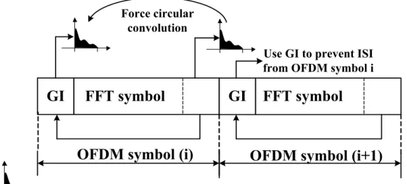
(21) However, OFDM system needs large number of sinusoidal oscillators to obtain orthogonal transformation until Weinstein and Ebert suggested using discrete Fourier transform (DFT) to replace the required oscillators, reducing implementation complexity of OFDM modem [16]. The OFDM modulation and demodulation by using Inverse DFT (IDFT) and DFT is shown as FIG 1.4. In realty, the IDFT/DFT is replaced by inverse fast Fourier transform (IFFT)/fast Fourier transform (FFT) with proper size to reduce hardware cost.. After IFFT, cyclic prefix (CP) will be added in front of the original FFT window as guard interval (GI) proposed by Peled and Ruiz. It makes the linear convolution with the channel impulse response similar to a circular convolution as FIG 1.5. Since circular convolution in time domain is equivalent to multiplication in the DFT domain. Orthogonality of subcarriers distorted by multi-path channel can be easily recovered with an equalizer to avoid ICI. The length of GI should be set longer than the expected delay spread of multi-path environment. Otherwise, ISI influence will exist. Force circular convolution. Use GI to prevent ISI from OFDM symbol i. GI. FFT symbol. GI. OFDM symbol (i). FFT symbol. OFDM symbol (i+1). : linear convolution with channel impulse response of OFDM symbol i FIG. 1.5 Use CP as GI to prevent ISI and maintain circular convolution 6.

(22) FIG 1.6 shows the simplified block diagram of OFDM transceiver. At first is FEC coder. It corrects the errors at weak subcarriers caused by frequency-selective-fading to reduce error probability. The trade off is the reduction of data rate by transmitting additional encoded data. Then QAM mapping increases the data rates of system, decreasing the noise margins of transferred as trade off. After QAM mapping, IFFT and GI insertion introduced previously complete the OFDM modulation.. Data In FEC Coder. I . QAM . S/P . Mapping Q .. I I . GI . IFFT . P/S Q Insertion Q .. I DAC Q. TX RF. Channel. Data Out. FEC Decoder. QAM I . . S/P De. Q . mapping. FFT. I I . GI . . P/S Q Remove Q .. I ADC Q. RX RF. FIG. 1.6 Simplified block diagram of OFDM system. 1.4 Outline of This Thesis In this thesis, Chapter 2 introduces the simulation platform and system specification, including IEEE 802.11a WLAN, LDPC-COFDM UWB system, and multi-band Viterbi COFDM (MB-OFDM) UWB system. The proposed algorithms according to different system requirements will be described in Chapter 3 and Chapter 4. In Chapter 3, we focus on a common throughput (less than 100MHz) frame synchronizer and use IEEE 802.11a WLAN for case study. In Chapter 4, we focus on a high throughput (greater than 500MHz) frame synchronizer and use LDPC-COFDM 7.

(23) and MB-OFDM UWB system for case study. The simulation result and performance analysis of our proposed design will be discussed individually in Chapter 5 for three different system platforms introduced in Chapter 2. Chapter 6 shows the architecture of proposed design and its hardware implementation result. Finally, conclusion and future work will be given in Chapter 7.. 8.

(24) CHAPTER 2 System Platform In this chapter, system platforms used for our case study will be introduced. The first is constructed according to IEEE 802.11a physical layer (PHY), finalized by IEEE 802.11 Wireless LAN committee in November 1999. It is an indoor wireless local area work (LAN) data communication in the 5GHz band. Others belong to OFDM based UWB system, including LDPC-COFDM system [8] and MB-OFDM system [7]. The system specifications of the two system platforms will be introduced individually.. 2.1 IEEE 802.11a PHY 2.1.1. System Platform. The system platform diagram of our IEEE 802.11a transceiver PHY is shown as FIG 2.1. The transmitter contains two main function blocks：OFDM modulation and forward-error correction (FEC) coding. The OFDM modulation has 64-point DFT with 4 kinds modulation methods listed in TABLE 2.1. The FEC coding supports three coding rates: 1/2, 2/3 and 3/4. The receiver contains three main function blocks: synchronization, OFDM demodulation and FEC decoding. Synchronization compensates the received signals degraded by channel effects. The detail channel effects will be discussed in section 2.3. After synchronization, the OFDM demodulation transfers time domain signals into frequency domain sub-carriers and FEC decoding corrects the error data caused by channel effects. 9.

(25) Data in. Convolutional Convolutional encoding encoding. scrambler scrambler. interleaver interleaver. FEC Encoding OFDM Modulation. QAM QAM mapping mapping RX RX RF RF. pilot pilot insertion insertion. I. ADC ADC. AGC AGC. ADC ADC. GI GI reduction reduction. I. Multi-path Multi-path Channel ChannelModel Model. Q. FFT FFT. De-interleaver De-interleaver. Preamble Preamble&&GI GI insertion insertion. IFFT IFFT. Q. Synchronization. Frame Frame detection detection. Channel Channel equalizer equalizer. Viterbi Viterbi decoding decoding. TX TX RF RF. AFC AFC. Phase Phase recovery recovery. QAM QAM de-mapping de-mapping. OFDM Demodulation. FEC Decoding De-scrambler De-scrambler. Data out. FIG. 2.1 IEEE 802.11a system platform. The major system parameters of IEEE 802.11a PHY are listed as TABLE 2.1. It required 20MHz bandwidth to transfer data. With 4 kinds modulations and 3 coding rates, the supported data rates are from 6M bits/s to 54M bit/s. The detail modulation parameters of supported data rates are listed as TABLE 2.2. For each transferred OFDM symbol, it has 48 data sub-carriers and 4 pilot sub-carriers, total 52 used sub-carriers modulated by 64–point FFT/IFFT. The last 16 points of IFFT outputs will be appended to the OFDM symbol as guard interval to retain the cyclic prefix property of FFT symbol. The performance requirement is less than 10% packet error rate (PER) according to the IEEE 802.11a SPEC.. 10.

(26) Required bandwidth. 20MHz. Date rate (Mbits/s). 6, 9, 12, 18, 24, 32, 48, 54. Modulation method. BPSK, QPSK, 16QAM, 64QAM. Error correct code. K=7(64 states convolutional code). FEC coding rate (R). 1/2, 2/3, 3/4. FFT size (N). 64. Number of used sub-carriers (NST). 52. Number of data carriers (NSP). 48. Number of pilot carriers (NSD). 4. OFDM symbol duration. 4.0 us. IFFT/FFT period (TFFT). 3.2 us. GI duration (TGI). 0.8us (TFFT/4). Packet Error Rate (PER) performance. ≦10%. TABLE 2.1 IEEE 802.11a PHY system parameters. Data rate. Modulation. (Mb/s). Coded. Coded bits. Coding. bits per. per OFDM per OFDM Required. Rate. subcarrier. symbol. symbol. (NBPSC). (NCBPS). (NDBPS). Data bits SNR. 6. BPSK. 1/2. 1. 48. 24. 9.7. 9. BPSK. 3/4. 1. 48. 36. 10.7. 12. QPSK. 1/2. 2. 96. 48. 12.7. 18. QPSK. 3/4. 2. 96. 48. 14.7. 24. 16-QAM. 1/2. 4. 192. 72. 17.7. 36. 16-QAM. 3/4. 4. 192. 144. 21.7. 48. 64-QAM. 2/3. 6. 288. 192. 25.7. 54. 64-QAM. 3/4. 6. 288. 216. 26.7. TABLE 2.2 IEEE 802.11a PHY data rate dependent parameters. 11.

(27) 2.1.2. Frame Format. FIG 2.2 shows the format of the PLCP protocol data unit (PPDU) used for IEEE 802.11a PHY. It comprises PLCP preamble, PLCP header and data field. The PLCP preamble is used for synchronization, including 10 short symbols and 2 long symbols. The short symbols are used for automatic-gain control (AGC), coarse timing detection and coarse frequency offset estimation. The long symbols are used for fine timing detection, fine frequency offset estimation and channel estimation. The detail PLCP preamble format and its timing parameters are shown in FIG 2.3 and TABLE 2.3. After the PLCP preamble is the PLCP header. It conveys information about coding rate, modulation type and the data length of PLCP service data unit (PSDU). The last component is data field contains variable number of OFDM symbols by the PSDU length.. PLCP header RATE Reserved LENGTH Parity Tail SERVICE. Coded/OFDM (1/2,BPSK). PLCP Preamble. PSDU. Tail. Pad. Coded/OFDM (indicated in SIGNAL). SIGNAL. DATA FIELD. FIG. 2.2 PPDU frame format of IEEE 802.11a PHY. PLCP preamble t1. t2. t3. t4. t5. t6. t7. t8. t9. t 10. Tshort : short training sequences. TGI2. T1. T2. TLONG : long training sequences. FIG. 2.3 PLCP preamble format 12. GI. SIGNAL OFDM symbol. GI. DATA OFDM symbol.

(28) TPREAMBLE: PLCP preamble duration. 16 us (TSHORT + TLONG). TSHORT: Short training sequence duration. 8 us (10 × TFFT/4). TLONG: Long training sequence duration. 8 us (TGI2 + 2 × TFFT ). t1~t10 : Short symbol duration. 0.8 us (10 × TFFT). T1~T2: Long symbol duration. 3.2 us (TGI2 + 2 × TFFT ). TGI2: Training symbol GI duration. 1.6 us (TFFT/2). TABLE 2.3 Timing parameters of PLCP preamble. 2.2 Ultra-Wideband System 2.2.1. System Platform. In recent years, UWB communication has received much attention as a high speed, low cost wireless LAN implementation in short distance. To promote UWB technology, FCC allowed spectrum from 3.1GHz to 10.6GHz, total 7.5GHz band for UWB devices in 2002. Since UWB system has not been standardized; two baseband systems has been proposed. One is impulse radio based, transmitting nano-second time domain pulses over a wide bandwidth [17~18]. The other is OFDM based, dividing spectrum into several sub-bands and use one OFDM modulation to transfer data. In this paper, we focus on two OFDM based UWB systems for case study. The first is LDOC-COFDM system, having 528MHz bandwidth, 128 point FFT, and low density parity check (LDPC) codec with 120Mb/s~480Mb/s data rates. The detail system spec and system requirement for 8% PER are listed in TABLE 2.4 and TABLE 2.5. The second is MB-OFDM system, transmitting OFDM symbols across three time-interleaved sub-bands. An example of 13.

(29) timing-frequency coding (TFC) for the MB-OFDM system is shown as FIG 2.4. TABLE 2.6 lists the SPEC of MB-OFDM system and TABLE 2.7 lists the system requirement for 8% PER.. Data Rate (Mb/s). FFT. Bandwidth (MHz). FEC Coding Rate Spreading Gain. 120. 128-point. 528. 3/4. 4. 240. 128-point. 528. 3/4. 2. 480. 128-point. 528. 3/4. 1. TABLE 2.4 LDPC-COFDM system SPEC. Data Rate (Mb/s) Required Distance (m) Required Eb/N0 (dB) Required SNR (dB) 120. 10. 12.91. 7.55. 240. 4. 18.35. 16. 480. 2. 20.5. 21.1. TABLE 2.5 Requirement for 8% PER of LDPC-COFDM system. Frequency: MHz 3168. 3696. pre-guard interval: 60.6 ns. OFDM symbol: 242.4 ns. guard interval: 9.5ns. Symbol Length 312.5 ns. 4224 4752. Band Period: 937.5 ns. FIG. 2.4 An example of MB-OFDM system for TFC (1、2、3、1、2、3) 14.

(30) Data Rate (Mb/s). FFT. Bandwidth (MHz). FEC Coding Rate Spreading Gain. 53.3. 128-point. 528. 1/3. 4. 80. 128-point. 528. 1/2. 4. 110. 128-point. 528. 11/32. 2. 160. 128-point. 528. 1/2. 2. 200. 128-point. 528. 5/8. 2. 320. 128-point. 528. 1/2. 1. 400. 128-point. 528. 5/8. 1. 480. 128-point. 528. 3/4. 1. TABLE 2.6 MB-OFDM system SPEC. Data Rate (Mb/s) Required Distance (m) Required Eb/N0 (dB) Required SNR (dB) 110. 10. 12.9. 7.1. 200. 4. 18.34. 15.2. 480. 2. 20.5. 21.1. TABLE 2.7 Requirement for 8% PER of MB-OFDM system. The system block diagram of OFDM based UWB system shown as FIG 2.5. It comprises transmitter, channel model and receiver. Transmitter sends transferred signals meet system SPEC. Channel model simulates channel interference and RF effects. At receiver, frame synchronizer detects the valid packet and FFT-window boundary. Then received signals are sent to demodulation, FEC decoder and finally it’s sent back to MAC. 15.

(31) Transmitter From MAC. LDPC encoder scrambler. QPSK. spreading. IFFT. convolutional encoder. preamble insert. clipping. Channel Model CFO. AWGN. frequency synchronizer. RF effects. Receiver. frame synchronizer AGC. timing offset. FFT. channel equalizer. DeQPSK. shaping filter. multipath channel. LDPC decorder. Descrambler. Viterbi decorder. To MAC. FIG. 2.5 System block diagram of OFDM based UWB system. 2.2.2. Frame Format. 1. Packet format :. PLCP preamble. PLCP header. Data. 9.375ns. 30 sync symbols 2. Preamble format :. 21 packet sync symbol. 3. Sync symbol format :. Pre - GI. 3 frame sync 6 Channel estimation symbol symbol. Sync Sequences (128 points ). Post -GI. FIG. 2.6 Frame format of MB-OFDM UWB system The Frame format of OFDM based UWB system is shown as FIG 2.6 [19]. One packet is constructed from PLCP preamble, PLCP header, and data field. The PLCP preamble duration is 9.375ns. It has 30 sync symbols, including 21 packet-sync symbols (PS), 3 frame-sync symbols (FS), and 6 channel estimation symbols (CES). One sync-symbol can be divided into pre guard 16.

(32) interval, sync sequences and post guard interval. The sync sequences have one hundred and twenty-eight points with constant amplitude (1 or -1). The pre guard interval is the cyclic prefix of sync sequences with 32 points. The guard interval is inserted for transmitter and receiver to switch the carrier frequency to next sub-band.. Transferred data. TX DAC CLK t1. SCO effect CLK t2. Received data. RX ADC. TX RF. multi-path fading channel. Carrier Freq. f1. CFO effect Carrier Freq. f2 Unpredicted Noise. RX RF. AWGN model. FIG. 2.7 Channel model data flow of simulation platform. 2.3 Simulated Channel Model The channel effects flow of our platforms in simulation are shown as FIG 2.7, including multipath fading channel, additive white Gaussian noise (AWGN), carrier frequency offset effect, and sampling clock offset (SCO) effect. We will introduce how these channel effects distorts the transferred data in detail as follows:. 17.

(33) 2.3.1 Multi-Path Fading Channel In wireless communication, the transmitting signals may collide with some obstacles and result other time-delay, power-decay reflected paths received by antenna. It is called multi-path interference, as shown in FIG 2.8. In time domain, the multi-path interference causes inter-symbol interference. (ISI). from. succeeding. symbols;. and. in. frequency. domain,. it. causes. frequency-selective fading when delay spread is longer than symbol period. In our platform, we model the multi-path interference by the linear convolution of corresponding channel impulse responses as. y (t ) = h(t ) ⊗ x(t ) = ∑ h(t − N∆ ) × x(t ) , h(t ) = impulse response N. . In IEEE 802.11a PHY, the channel impulse response is established from the IEEE 802.11a channel model [20]. An example of the IEEE channel impulse response for 100 ns RMS delay spread is shown in FIG 2.9. In UWB system, we use Intel channel model [21] for LDPC-COFDM system and IEEE 802.15.3a channel environment from CM1 to CM4 model [22] for MB-OFDM system. FIG 2.10 shows an example of the UWB channel impulse of Intel channel model for 9ns RMS delay spread. Impulse reseponse. obstacle 1. ISI effect path (i-1). TX RF. path i path (i+1). obstacle 2. path (i-1). RX RF. path i path (i+1). GI GI. FFT symbol FFT symbol GI. GI. FFT symbol. FIG. 2.8 Multi-path interference and ISI effect 18. GI. FFT symbol FFT symbol GI. FFT symbol.

(34) FIG. 2.9 IEEE 802.11a channel impulse response. FIG. 2.10 UWB channel impulse response 19.

(35) 2.3.2 AWGN Model At receiver antenna, the transferred signals will be interfered by non-predicted noise. In our platform we use AWGN model to simulation the non-predicted noise. The AWGN signal w(t) is generated by MATLAB as follows:. w(t ) = rand (1, L ) × RMS + j × rand (1, L ) × RMS Where L is the length of data signals and RMS is the normalized root mean square power defined as:. RMS = 10. ( Pdata − SNR ) / 20. 2. Where Pdata is the power of data signal ands SNR is the SNR ratio between data signals and AWGN signals.. 2.3.3 Carrier Frequency Offset Model Carrier frequency offset (CFO) is happened due to the difference of carrier frequency between transmitter RF and receiver RF. The CFO effect in time domain can be represented as follows:. y (t ) = x(t ) × e − j×2π ( f1 − f 2 )T ×t Where f1 is the carrier frequency of transmitter and f 2 is the carrier frequency of receiver. The parameter T is the period of sample clock. In IEEE 802.11a PHY, the sample clock rate is 20MHz and T equals to 50ns. In OFDM-based UWB system the sample clock rate is 528MHz and T equals to 1.894ns .It clearly shows CFO effect will cause linear phase shift in time domain as Fig 2.11. 20.

(36) FIG. 2.11 Linear phase shift caused by CFO With the linear phase shift in time domain decaying the orthogonality of subcarriers, CFO induces inter-carrier interference (ICI) in frequency domain by moose’s law [23]. ICI effect can be represented as follows： ⎤ • exp( jπ∆f ( N Y [k ] = H [ k ] X [ k ] × ⎡sin (π∆f ) FFT − 1) N FFT ) N FFT • sin (π∆f N FFT )⎥⎦ ⎢⎣. ⎡ ⎤ ⎢ ⎥ ⎥ • exp( jπ∆f ( N FFT − 1)) • exp( jπ ( m − k )) + ∑ H [ m ] X [ m ] × ⎢sin (π∆f ) ⎞ ⎛ ∆ + − π ( ) f m k ⎢ ⎥ N FFT N FFT m=− k ⎟⎟ ⎥ N FFT • sin ⎜⎜ m≠k ⎢ N FFT ⎠⎦ ⎝ ⎣ k. ICI. 2.3.4 Sampling Clock Offset Model As shown in FIG 2.7, sample clock offset (SCO) is caused by the variances of sampling frequency between digital to analog converter (DAC) in transmitter and analog to digital converter (ADC) in receiver. In time domain, SCO results time shift from practical sampled points and ideal 21.

(37) sampled points. Without compensating SCO effect, the time shift error will be accumulated. It leads ADC to sample the received signal at wrong time and fails receiver behavior. The SCO distortion also makes a linear phase error in frequency domain as FIG 2.12. Thus, we use pilot sub-carriers to estimate the linear phase error caused by SCO to recovery the transferred data.. FIG. 2.12 SCO effect in Time domain and frequency domain 22.

(38) CHAPTER 3 A Low Complexity Frame Synchronizer for OFDM Application In this chapter, a low complexity frame synchronizer used for OFDM system is proposed. It mainly chooses the most-significant taps of matched filter used for FFT window detection to reduce correlation complexity of frame synchronizer. To explain our study clearly, the IEEE 802.11a PHY introduced in chapter 2 is selected as our system platform. The detail algorithm, analysis and simulation results will be shown in the following.. 3.1 Frame Synchronizer Data Flow Frame Synchronizer Long Preamble Detection From ADC. FFT Window Detection. Packet Detection. Fine AFC. To FFT. Coarse AFC. FIG. 3.1 Frame synchronizer data flow. The data flow of proposed frame synchronizer is shown in FIG 3.1. In the initial, packet detection detects the valid packet through normalized auto-correlation algorithm in short preamble. A decision threshold is chosen to compare with the normalized auto-correlation value. The valid 23.

(39) packet will be asserted when the normalized auto-correlation value is greater than decision threshold. Then, coarse frequency compensation uses residue short training symbols to compensate CFO ≦ ±4ppm(±20KHz). At the same time, frame synchronization detects the end of short preamble by another decision threshold. Next, FFT window detection finds out start boundary of FFT window by comparing with one long training sequence (cross-correlation algorithm).. After deciding the FFT window boundary, fine frequency compensation compensates. remain CFO ≦ 0.8ppm(4KHz) and channel equalizer estimates channel response by another long training sequence.. 3.1.1 Packet Detection In 802.11a PHY, the valid packet can be detected by depending the periodic data property of PLCP preamble. As mentioned in 2.1.2, short preamble is constructed by ten repeating short symbols and each short symbol has period ‘Ts’ (0.8us). Thus we make a comparison of received signals R(t) and R(t+Ts) by the normalized auto-correlation scheme [24-25] depicted as follows: N −1. C k = ∑ rk + m × r(*k + m )+ N m =0. N −1. Pk = ∑ r( k + N + m ). 2. m=0. λk =. 2. Ck Pk. 2. (Eq 3.1). In the above equation: Ck is the auto-correlation value and Pk is the corresponding symbol power. The parameter ‘N’ is the number of sample points in a short period ‘Ts’ equaling to 16. 24.

(40) Normalizing the auto-correlation value Ck with symbol power Pk , we can get a new decision value. λk. The normalized auto-correlation valueλk can detect the valid packet independent with receiver power level. Thus packet detection begins working without AGC turning the correct RF receiver gain. In IEEE 802.11a PHY, AGC, packet detection, diversity selection and Coarse CFO estimation are required to be complete in short preamble duration. The number of short symbols needed for packet detection should be as less as possible. In our design, since AGC and packet detection can work simultaneously, they can share short symbols with each other and get longer estimation time to increase performance. The proposed decision value Λ k are defined as following equation: it uses three short symbol pairs for normalized auto-correlation algorithm.. Λ. k. =. C k + C k −1 + C k − 2. 2. ( Pk + Pk − 1 + Pk − 2 ) 2. FIG. 3.2 Example of Packet Detection in Proposed Design 25. (Eq 3.2).

(41) FIG 3.2 shows an example of packet detection. Noise signals with 5us are added before the valid packet. The testing channel condition is SNR=0dB, CFO=200KHz(40ppm) and multipath delay spread=150 ns. The vertical axis is the proposed normalized auto-correlation value Λk. To detect the valid packet, a pre-defined threshold is needed to compare with Λ k. Once the normalized correlation value is greater than pre-defined threshold, detection of packet will be asserted. It is clearly under low SNR regions, the normalized auto-correlation value of noise signal varies extremely. To reduce the error rate of false announcement, a decision window is defined to test packet assertion. When Λk is greater than pre-defined threshold, the decision window starts to check the following correlation values. Packet detection only announce when all correlation values in decision window are also greater than the pre-defined threshold. If not, the packet assertion will be canceled and packet detection returns the initial state, as shown in FIG 3.2. .. 3.1.2 FFT Window Detection In our proposed design, FFT window detection finds the correct FFT window boundary by the known-data property [26]. It compares the received data with the ideal long training symbol data in a pre-defined searching window. The data comparison is based on the cross-correlation algorithm shown as follows：. ∆(k ) =. Ln −1. ∑ n =0. 2. R( k +n ) × Cn*. (Eq 3.3). In the above equation, ‘R’ is the received data from ADC, ‘C’ is the corresponding compared element of long training symbol. ‘Ln’ is the total number of elements in one long training symbol. In 802.11a standard, Ln is the same as FFT size equaling to 64. Δ(k) is correlation value of the 26.

(42) kth index of pre-defined searching window. Thus the maximum cross-correlation value represents which most similar to the ideal long training symbol, declared as the FFT window boundary.. FIG. 3.3 FFT window detection in AWGN and multi-path channel. 27.

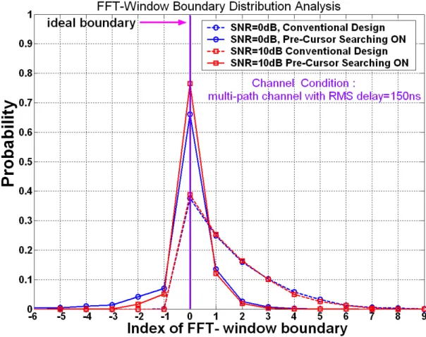
(43) An example of FFT window detection in AWGN channel and multi-path channel with 150 ns RMS delay spread is shown as FIG 3.3. It is clearly in the AWGN channel, the maximum cross-correlation index will be the start of FFT window as we expected. However in the multi-path channel, the delay spread of other arrival paths makes the maximum cross-correlation value locate in the later samples compared with the ideal FFT window boundary, and the correct FFT window boundary becomes the 2th or 3th peak cross-correlation value in the searching window. A common resolution is choosing the index earlier N points (N is an integer modified by designer) than the maximum cross-correlation value index as preferred FFT window boundary. However, the early catching will reduce the effective GI and degrades system performance in severe multi-path channel [27]. To solve this problem, the TOP ‘M’ pre-cursor searching scheme in [3] was referenced. It defines the index of maximum ‘M’ cross-correlation values as boundary candidates. The ‘N’ samples before the peak cross-correlation value is pre-cursor window. If there are more than one boundary candidates locating in the pre-cursor window, chooses the earlier index as our preferred FFT window boundary. Otherwise, chooses the peak cross-correlation value index as our preferred FFT window boundary. FIG 3.4 is the FFT window boundary distribution between using pre-cursor searching scheme (In our design, M=5 and N=5) and conventional design (without pre-cursor searching scheme) in multi-path channel with RMS delay spread=150 ns. For the perfect boundary cutting (index=0 at FIG 3.4), using pre-cursor searching scheme has correct probability twice the conventional design. Also the boundary distribution of pre-cursor searching scheme is more centralized, meaning less early catching points needed to retain effective GI. Comparing the simulation curves in SNR=0dB and SNR=10dB, since increasing SNR can’t reduce 28.

(44) multi-path interference, the boundary distribution of conventional design choosing the maximum correlation value in different SNR region are almost the same. However, SNR improvement can reduce probability of error boundary candidates in pre-cursor searching scheme caused by AWGN noise. Thus SNR improvement of pre-cursor searching scheme leads to better boundary distribution centralization (index=0) and less early catching (index from –4 to -1).. FIG. 3.4 FFT window detection in AWGN and multi-path channel. 3.2 Proposed Algorithm 3.2.1 Most-Significant Taps Scheme In 802.11a PHY, the most hardware cost of frame synchronizer is FFT-window detection. To 29.

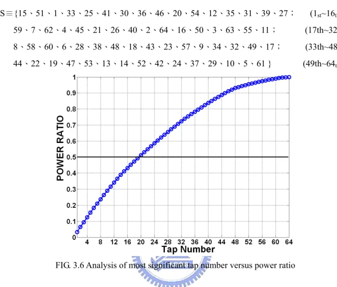
(45) implement the cross-correlation scheme (Eq 3.3), matched filter with 64 taps are used to calculate the timing metric Δ(k), meaning 64 complex multipliers(each complex complier has four multipliers and two adders) are needed. Therefore, the most efficient approach for hardware saving is reducing required taps compared in FFT window detection. However, matched filter is based on ML estimation, its compared accuracy has positive relation with input data power. And decreasing tap number of matched filter may result in performance degradation. To reduce required taps of matched filter with the least performance loss, the most-significant taps schemes is proposed.. ∆(k ) =. N. ∑ m=1. 2. R( k + S [ m ]) × CS*[ m ]. (Eq 3.4). In Eq 3.4, the parameter C is the matched-filter coefficient from C0 to C63, corresponding to the 64 taps. S is the index-sorting matrix from the maximum element of C to the minimum element. For example, S[1] represents index of the 1st maximum element of C and S[2] represents index of the 2nd maximum element. The parameter N is the number of used taps modified by user in demand. FIG 3.5 shows the power distribution of matched-filter coefficients in time domain and reorders them by power ratio.. FIG. 3.5 Power distribution of C0~C63 and S[1]~S[64] 30.

(46) The contents of index-sorting matrix S is listed as follows: S≣{15、51、1、33、25、41、30、36、46、20、54、12、35、31、39、27；. (1st~16th). 59、7、62、4、45、21、26、40、2、64、16、50、3、63、55、11；. (17th~32th). 8、58、60、6、28、38、48、18、43、23、57、9、34、32、49、17；. (33th~48th). 44、22、19、47、53、13、14、52、42、24、37、29、10、5、61 }. (49th~64th). FIG. 3.6 Analysis of most significant tap number versus power ratio. In 802.11a standard, the matched-filter coefficients are generated from the long OFDM training symbol transferred into time domain, resulting great power ratio variance between the coefficients. In the most-significant taps scheme, the least power ratio coefficients will be seen as redundant taps and removes from matched-filter. Thus the most-significant taps scheme can reduce correlation-complexity with less performance degradation. FIG 3.6 plots the total number of taps used for most-significant taps scheme versus its containing power ratio. The matched filter in [28] proposed using first 32 matched filter coefficients for low-power synchronizer design. It has 50 % power ratio from the conventional design (with total 64 taps). However in most 32 significant taps scheme, 50% correlation complexity from conventional 64 taps is saved as [28] with 32 taps, but 31.

(47) the proposed design still containing 72.4% power ratio from conventional design. Therefore it can get better performance than [28]. On the other hand, the most significant taps scheme only requires 20 taps to reach 50% power ratio, saving 37.5% complexity from [28].. 3.2.2 Quantization Approach Another effective approach to reduce complexity of cross-correlation was proposed in [29]. The proposed correlation scheme quantized the matched filter coefficients into the value composed of {0、±20、±2-1 、±2-2 ……±2-q }. By the quantized 2-q - level coefficients, multiply function of cross-correlation scheme can be replaced with q-bit shifting function. Thus multipliers used for correlation can be simplified into q-bit shifters. In IEEE 802.11a standard, the time domain long training symbol can be quantized into {0、±2-3、±2-4、±2-5、2-6 }. The drawback of this approach is serious quantization error, as FIG 3.7 shown.. FIG. 3.7 Tap power analysis of quantized approach 32.

(48) We use signal to quantization error ratio (SQNR) to estimate the quantization error (Eq 3.5)： 2 64 ⎫ ⎧ Cm ⎪ ⎪ ∑ ⎪ ⎪ m =1 SQNR = 10 log ⎨ 2⎬ 64 ⎪ (Cm − Qm) ⎪ ⎪⎭ ⎪⎩ ∑ m =1. (Eq3.5). Parameter C is the original matched filter coefficient and Q is coefficient after quantized. The SQNR of quantization approach is 14.86dB. Although the SQNR ratio is some worse, FIG 3.8 shoes the FER simulation in multipath channel with 150 ns RMS delay spread and CFO =100KHz under perfect packet detection. The SNR loss between original 64 taps and quantized 64 taps is only 0.5 dB for 1% FER.. FIG. 3.8 FER between conventional and quantization approach 33.

(49) Finally, we proposed a low complexity cross-correlation design for FFT-window detection by combining the most-significant taps scheme and the quantization approach. The algorithm is shown as follows:. ∆(k ) =. N. ∑ m =1. 2. R( k + S [ m ]) × QS*[ m ]. QX = arg min T {Re[C X ] − T } + j × arg min T {Im[C X ] − T } T ∈ {0,±2 −3 ,±2 −4 ,±2 −5 ,±2 −6 }. (Eq 3.6). S ≡ index sortting matrix of most − significant taps scheme Similar to Eq 3.4, parameter ‘R’ is the received signals and ‘N’ is the number of used taps. The parameter ‘N’ to reduce complexity while still maintaining performance is different with channel condition and user’s concern. In chapter 5, we will show the simulation results between channel model, complexity, and performance in our 802.11a system platform.. 34.

(50) CHAPTER 4 A Low Complexity and High Throughput Frame Synchronizer for OFDM-Based UWB System In this Chapter, a novel frame synchronizer is proposed for OFDM-based UWB system. Integrating the tap-reduction scheme, register-sharing algorithm and dynamic threshold, the proposed design can save over 50% area cost and power consumption from the conventional design power with an acceptable performance loss. Moreover, the proposed design can achieve 528MS/s throughput for 120~480Mb/s data rates UWB system in 0.18µm CMOS process.. 4.1 Motivation For OFDM-based UWB system, Frame synchronizer requires over hundreds of Mega samples per second throughput. Conventional frame synchronizer using single matched filter is not efficient to achieve high throughput by the long critical path of complex multiplier used for matched filters. On the other hand, parallel approaches with multiple matched-filters [9-10] to achieve such high throughput will lead to high area cost and high power consumption. To solve this problem, reducing matched filter complexity becomes the main concern to implement our design. In a matched-filter, tap number and required throughput dominate design complexity. Thus we proposed a tap-reduction scheme to reduce tap number for low-complexity improvement. Furthermore, another register-sharing algorithm cooperates with the tap-reduction scheme to save required size of register-files for parallel architecture. Finally, dynamic threshold design is adopted 35.

(51) to enhance frame error rate performance from the conventional fixed-threshold design. The platform of our OFDM-based UWB system has been introduced in section 2.2. In the following, we first introduce the proposed algorithm based on LDPC-COFDM system to reach 528MS/s high throughput, including tap-reduction scheme, register-shaing algorithm, and dynamic threshold design. Then we apply the proposed algorithm for MB-OFDM system and add another dynamic searching window algorithm to detect RF switching of the three time-interleaved sub-bands. The performance analysis and simulation result of proposed design will be shown in chapter 5.. 4.2 LDPC-COFDM Design In LDPC-COFDM system, transmitter sends the valid data at one fixed sub-band with 528MHz bandwidth. Without time-interleaving the OFDM symbols, the TFC of RF will maintain constant. Thus frame synchronizer needn’t to consider the correct switching time between the sub-bands.. 4.2.1 Frame Synchronizer Flow FIG 4.1 is the data flow of proposed frame synchronizer for LDPC-COFDM UWB system. In the initial, Packet detection detects the valid packet from the received signals through auto-correlation scheme. After packet announcement, FFT window detection finds the correct FFT window boundary by matched filters. Then preamble timing detection distinguishes three kinds of sync symbols (PS, FS, CES) in preamble. Finally, by the control signals from three main blocks, FFT symbol gate cuts OFDM data symbols to FFT for frequency domain transformation. 36.

(52) FFT Window Detection. Packet Detection. Preamble Timing Detection. Preamble Cut. Boundary Cut Packet Announce. FFT Symbol Gate. From ADC. To FFT. FIG. 4.1 Frame synchronizer flow. 4.2.1. 1 Packet Detection Noise signals and valid packet will be distinguished by using periodic packet sync symbols. The normalized auto-correlation scheme of packet detection is shown as follows: N −1. AX = ∑ rX *N +n × r(*X +3)*N +n n =0. N −1. PX = ∑ r( X + 3)* N + n n =0. λX =. AX PX. 2. (Eq 4.1). 2 2. In Eq 4.1, the parameter ‘r’ is the received signals from ADC. Before valid packet announcement, the received signals will be divided into several received symbols with 312.5ns time duration (equal to one OFDM symbol duration). The parameter ‘X’ is the index number of the received symbols, and ‘N’ is the total length of samples in one received symbol. The calculated result ‘AX’ represents the auto-correlation value of the Xth received symbol, ‘PX’ represents the 37.

(53) power estimation of Xth received symbol, and λ X represents the normalized auto-correlation value of Xth received symbol. In [30], it proposed that AFC estimates CFO effect by the phase of auto-correlation value for OFDM symbol pair with three symbols duration. To share auto-correlation value with AFC, packet detection calculate auto-correlation value between received symbol Xth and (X+3)th as FIG 4.2. Moreover, to prevent false announcement, packet detection asserts the valid packet at index k when both λ X and λ X −1 are higher than the pre-defined threshold.. threshold compare. λ2. λ1. X =1. threshold compare. threshold compare. X =2. λ3. X =3. threshold threshold compare compare. λ4. X =4. λ5. X =5. λ6. X =6. X =7. X =8. X =9. 312.5ns. FIG. 4.2 Packet detection flow. 4.2.1. 2 FFT Window Detection After packet detection, FFT Window detection finds FFT window boundary by comparing sync sequences in packet sync symbol. It also based on the cross-correlation algorithm and matched-filter. Section 2.2.1 refers that sync sequences has 128 points. Thus the tap number of matched-filter is 128. The cross-correlation algorithm is shown as follows：. 38.

(54) 2. Ls −1. Λ(m) = ∑ r( m+n ) × sn*. (Eq 4.2). n=0. In Eq 4.2, parameter ‘r’ is the received data from ADC, ‘s’ is the corresponding sync sequences used as matched-filter coefficients, ‘Ls’=128 is the total tap number, and ‘m’ is the index of pre-defined searching window with 312.5ns time duration (equal to one OFDM symbol duration).. 4.2.1. 3 Preamble Timing Detection In the proposed frame synchronizer, FFT window detection only finds the FFT window. We still need preamble timing detection to divide preamble from received data. The decision scheme of preamble timing detection is shown as follows: Ls −1. DY = ∑ rY *N +n × r(*Y +1)*N +n n =0. PY =. L s −1. ∑ r(Y +1)*N + n. 2. ( Eq 4.3 ). n=0. DY + DY −1 ≥ Γ × (PY + PY −1 ) 2. 2. In the above equation, ‘DY’ is the auto-correlation value of the sync sequences in Yth packet sync symbol, ‘PY’ is the corresponding symbol power, and ‘Ls’=128 is the total points in sync sequences. Preamble timing detection is also based on the auto-correlation scheme and ‘Γ’ is the parameter of compared threshold. From the proposal [19], frame sync symbol equals packet sync symbol multiplying –1. The auto-correlation value between the last packet sync symbol and first frame sync symbol will be negative to auto-correlation value of other sync symbol pairs. Thus 39.

(55) preamble timing detection decides first sync symbol by Eq 4.3 shown as FIG 4.3. Since before preamble timing detection, FFT window boundary has been detected. We can remove cyclic prefix interfered by ISI from sync symbols and only use sync sequences for correlation estimation.. threshold compare. threshold compare. threshold compare. threshold compare (eliminate and approach zero). D. D. 17th PS. 18th PS. D. D. 19th PS. 20th PS. -D 21th(last) PS. 1st FS. FIG. 4.3 Preamble timing detect flow. 4.2.2. Proposed Algorithm. 4.2.2. 1 Tap-Reduction Scheme As mentioned earlier, parallel approaches to achieve 528MS/s throughput leads to high hardware cost and power consumption. For low complexity improvement, reducing tap number of matched filter was proposed [10]. The trade off is performance degradation of frame synchronizer. According to the UWB system proposal [19], the power of sync sequences is constant for every sample point. We can’t apply the most-significant taps scheme introduced in section 3.2.1 to reduce tap number of matched filter. Therefore, we proposed a tap-reduction scheme to reduce correlation complexity by down sampling the received signals because of the average power distribution property of sync sequences. The proposed tap-reduction scheme can also apply for 40.

(56) auto-correlation scheme. In the following, we show the modified functions of Eq 4.1~ Eq 4.3： Packet Detection： ⎣( N −1) / w ⎦. ∑. AX =. n =0. rX *N +n×w × r(*X +3)*N +n×w. ⎣( N −1) / w ⎦. ∑. PX =. r( X +3)*N + n×w. n =0. λX =. 2. AX PX. 2. ( Eq 4.4 ). 2. FFT Window Detection：. Λ(m) =. 2. ⎣( Ls −1) / w⎦. ∑ n=0. r( m+n×w) × sn*×w+ j. ( Eq 4.5 ). Preamble Timing Detection：. DY =. PY =. ⎣( Ls −1) / w ⎦. ∑ n =0. rY *N +n×w × r(*Y +1)*N +n×w. ⎣( L s −1) / w ⎦. ∑ n =0. r(Y +1)* N + n× w. ( Eq 4.6 ). 2. DY + DY −1 ≥ Γ × (PY + PY −1 ) 2. 2. In Eq 4.4 ~Eq 4.6, the parameter ‘ω’ is a reduction factor controlling correlation complexity and tap number for each function block.. Differing from conventional down-sampling scheme having only 1/‘ω’ throughput rate of input data, the tap-reduction scheme still has the same throughput rate (528MS/s) with input data to keep timing resolution of FFT window detection. Sync sequences used as matched-filter taps. 41.

(57) are also divided into ‘ ω ’ groups ( S n×w+ j. j ∈ {0, 1, 2...., w − 1} ). By the average power. distribution property of sync sequences, any one of the ‘ω’ groups chosen as matched-filter taps has equal performance. The detail performance simulation of tap-reduction scheme will be shown in section 5.2.1. By the simulation result, we proposed ‘ω’=4 for our frame synchronizer. The data flow of conventional design and design using tap-reduction scheme (with ‘ω’=4, ‘j’=3) are shown in the following：. Register file: with 128 words. Received samples. 0. 1. 2. 3. ……………. 124 125 126 127. m=0. Compared 0 Taps. Received samples. 1. 1. 2. 3. ……………. 124 125 126 127. 2. 3. 4. ……………. 125 126 127 128. m=1. Compared 0 Taps Received samples. 2. 1. 2. 3. ……………. 124 125 126 127. 3. 4. 5. ……………. 126 127 128 129. m=2. Compared 0 Taps. Received samples. 3. 1. 2. 3. ……………. 124 125 126 127. 4. 5. 6. ……………. 130 131 132 133. m=3. Compared 0 Taps. 1. 2. 3. ……………. 124 125 126 127. Received samples has been stored by register files 0. 1. 2. 3. 4. 5. 6. 7. …… 127 128 129 130 131 132 133 …… 127+(N-1). FIG. 4.4 Data flow of conventional design with 128 taps (w=1). 42.

(58) Register file: with 32 words Received samples. 0. 4. 8. 12. ……………. 112 116 120 124. m=0. Compared 3 Taps Received samples. 7. 1. 11 15. 5. 8. 13. ……………. 115 119 123 127. ……………. 113 117 121 125. m=1. Compared 3 Taps Received samples. 2. 7. 11 15. ……………. 115 119 123 127. 6. 10 14. ……………. 114 118 122 126. m=2. Compared 3 Taps Received samples. 3. 7. 11 15. ……………. 115 119 123 127. 7. 11 15. ……………. 115 119 123 127. m=3. Compared 3 Taps. 7. 11 15. ……………. 115 119 123 127. Received samples has been stored by register files 0. 1. 2. 3. 4. 5. 6. 7. …… 127 128 129 130 131 132 133 …… 124+(N-1). FIG. 4.5 Data flow of tap-reduction scheme with 32 taps (w =4, j =3). FIG 4.4 is the conventional design with 128 taps (‘ω’=1). The register-files storing received samples for cross-correlation are 128 words. FIG 4.6 is the tap-reduction scheme with 32 taps (‘ω’=4 ‘j’=3). Comparing FIG 4.4 and FIG 4.5, tap-reduction scheme reduces 75% correlation complexity and register-files length of conventional design from 128 taps to 32 taps. However, when applying parallel architecture for high-throughput matched-filter design, the register-files should be parallelized, too. To resolve the increasing size of register-files for parallelism, we proposed another register-sharing algorithm. It can cooperate with the tap-reduction scheme to share received samples for the parallel matched-filters to reduce required size of register-files. 43.