適用於三維積體電路之線性規劃

國立交通大學

電子工程學系 電子研究所碩士班

碩 士 論 文

適用於三維積體電路之線性規劃

Generic Integer Linear

Programming Formulation for 3D IC

Partitioning

研究生：梅宗菀

指導教授：江蕙如 博士

適用於三維積體電路之線性規劃

Generic Integer Linear Programming Formulation for 3D IC

Partitioning

研究生：梅宗菀

Student: Tsung-Wan Mei

指導教授：江蕙如 博士

Advisor: Dr. Iris Hui-Ru Jiang

國立交通大學

電子工程學系 電子研究所碩士班

碩士論文

A Thesis

Submitted to Department of Electronics Engineering & Institute of

Electronics College of Electrical and Computer Engineering

National Chiao Tung University

In Partial Fulfillment of the Requirements

For the Degree of

Master

In

Electronics Engineering

February 2011

Hsinchu, Taiwan, Republic of China

中華民國 一○○年二月

適用於三維積體電路之線性規劃

研究生：梅宗菀 指導教授：江蕙如 博士

國立交通大學

電子工程學系 電子研究所

摘要

Generic Integer Linear Programming Formulation for 3D

IC Partitioning

Student: Tsung-Wan Mei Advisor: Dr. Iris Hui-Ru Jiang Department of Electronics Engineering

Institute of Electronics National Chiao Tung University

Abstract

As technology advances, 3D IC has gradually become a trend, because it is a novel technology, it requires new EDA technology, and partitioning is one of important items. This paper targets on partitioning from the architectural level, in order to maximize its benefit. First, we use the logical operators to solve the problem of 3D IC partitioning, and converted into integer linear programs (ILPs). Our ILP formulation can reduce the number of TSV and power, and because of its flexibility, it can be expanded to support multiple supply voltage designs. We propose two methods to speed up the ILP computation, Experimental results show that our method can effectively reduce the ILP computation time. In addition, our method also has great flexibility in space, by restrictions on changes or new ILP formula can easily be extended to different target partitioning problem. This flexibility makes the ILP formula we can easily solve the general 3D IC partitioning problem.

Acknowledgements

I would like to express my heartfelt gratitude to all those who gave me the possibility to complete the thesis. First of all, my sincerest appreciation goes to my advisor, Prof. Iris Hui-Ru Jiang, for her patient guidance and spur throughout my graduate course. Then, I would like to be grateful to the members of my thesis committee, Prof. Mango Chia-Tso Chao and Prof. Charles Hung-Pin Wen, for their precious suggestions and comments. Meanwhile, I deeply appreciate Wan-Yu, and members of IRIS Lab, Yen-Ting, Yu-Ming, Ya-Chung. Also, I deeply show my appreciation to my parents and friends for their invaluable support throughout my study years.

Tsung-Wan Mei

National Chiao Tung University February 2011

Table of Contents

Abstract (Chinese) i

Abstract ii

Acknowledgements iii

List of Tables vi

List of Figures vii

Chapter 1 Introduction 1 1.1 Background ……….. 1 1.2 Previous Work ………. 5 1.2.1 Partitioning ……….. 5 1.2.2 ILP Formulation ……….. 6 1.3 Thesis Organization ………. 7 Chapter 2 Preliminaries 8 2.1 Vertical Interconnects ……….. 8

2.2 Multilevel Multi-way Partitioning ……….. 9

2.3 Multiple Supply Voltage (MSV) ……….. 10

Chapter 3 Generic ILP Formulation for 3D IC Partitioning 11 3.1 Problem Definition ……….. 11 3.2 Hypergraph Modeling ……….. 12 3.3 ILP Formulation ……….. 13 3.4 ILP Reduction ……….. 15 3.4.1 Iterative ILP ………. 15 3.4.2 Pre-clustering ……… 16 iv

Chapter 4 An Extension to MSV Design 17

4.1 Problem Definition ……….. 17 4.2 Extended ILP Formulation for MSV Design ……….. 18 4.3 Speed-up ……….. 20

Chapter 5 Experimental Results 21

5.1 Generic ILP vs. Iterative ILP ………... 22 5.2 ILP with MSVs ………... 24

Chapter 6 Conclusion 30

6.1 Concluding Remarks ………... 30

Bibliography 31

List of Table

3.1 Variables used in our generic ILP formulation ……… 14

3.2 Logical expressions vs. mathematical constraints ……… 14

4.1 Variables used in our extended ILP formulation for MSV design ……... 19

5.1 Statistics on GSRC benchmarks ……….. 21

5.2 Results on GSRC benchmarks with single voltage ……….. 23

5.3 Results on GSRC benchmark with MSV ………. 25

List of Figures

1.1 A 3D IC with TSVs for vertical interconnects

(via first, front to back integration) ……….. 1

1.2 Conventional multi-way partitioning in (a) cannot guarantee optimality in 3D IC integration in (b) ……….. 3

1.3 The process of Partitioning algorithm ………. 5

1.4 The flow chart of Partitioning program ……… 6

2.1 The three phases of hMetis ……….. 9

3.1 3D IC partitioning ……… 11

3.2 The iterative ILP algorithm ……….. 15

5.1 Comparisons of (a) #TSVs and (b) runtime between iterative ILP w/ and w/o MSV ………. 27

5.2 Comparisons of (a) #TSVs and (b) runtime between iterative ILP w/ pre-clustering and w/o pre-clustering ……….. 28

5.3 Comparisons of (a) #TSVs and (b) runtime between iterative ILP with MSV w/ pre-clustering and w/o pre-clustering ……….. 29

1

Chapter 1

Introduction

1.1

Background

Technology Roadmap for Semiconductors (ITRS)預測，隨著光學蝕刻技術越接 近自然極限，增加規模整合是必須的[5]。圖 1.1 表示了一個三維積體電路使用 through-silicon vias (TSVs)去連接各層的設備層和金屬層。而連接層(bonding layer)則是層與層之間的黏合劑。從各方面看來，儘管三維積體電路是可行也有

layer 3

layer 2

layer 1 Stacked die

Bulk silicon (substate wafer) Heat sink Encapsulation TSV cell Landing pad Interlayer dielectric Metal layers Device layer TSV IO Bump TSV through (bonding layer)

Figure 1.1 A 3D IC with TSVs for vertical interconnects (via first, front to back integration) [3].

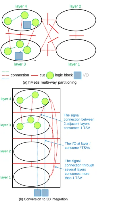
2 益的，但在 IC 上打 TSV 過程的變化(11.1%)遠遠大於閾值電壓裝置的變化 (6.4%)，因此，TSVs 應該要更精巧地被使用。 而要將一般平面電路轉換成三維結構需要新穎和自動化的設計，分割電路就 是一項很重要的技術，因為其結果會大大影響電路的 performance。另一方面， 決策和優化在一個更高的層級比起工作在較低的層級能得到更多優點。例如，從 結構層級的功能分割比起從物理層級分割能得到更多的好處，因為功能分割可以 適當的連接功能和操作（logic blocks）之間。從功能分割的設計上除錯比起從 電路上除錯也要容易得多。此外，在結構層級問題的大小明顯小於在物理層級， 即數位邏輯閘，通常不超過一百個。本文著重從結構層級將電路分割為三維積體 電路結構。這種方法可以很容易地擴展到所有的層級。在這篇論文裡，三維積體 電路的每層為一設備層加一金屬層組成，相當於一個分區（堆疊）。以前的研究 表示最大限度地減少切割的大小可以間接地優化繞線長度 [6] [7]。因此，良好 的分割演算法可能使得後期階段有更好的解決方案。 由於三維積體電路所有的相互作用與外部信號進行只能通過最底層，三維積 體電路分割問題是相當不同於傳統之一。如圖 1.2(a)所示，傳統的電路分割演 算法，例如 hMetis[8]，不能保證是最好的方法。從單純的基礎上擴展到傳統的 電路分區，每個分區後，假若被分配到三維積體電路的一組不同的設備層和金屬 層，如圖 1.2(b)所示，一個被切割或連接一個輸入/輸出（I/ O）的 net，其相 關的 pin 點可能剛好分散在多個非相鄰層時，就有可能需要使用超過一根 TSV 來 做連接。因此，最少的 cutsize 電路分割不能很好地反映如何減少使用 TSV 的數 量。此外，安排這些分區是不簡單的。

3 … layer 1 layer 2 layer 3 layer 4 I/O cut logic block

connection

(a) hMetis multi-way partitioning

layer 1 layer 3

layer 2 layer 4

(b) Conversion to 3D integration

The I/O at layer i consume i TSVs The signal connection between 2 adjacent layers consumes 1 TSV The signal connection through several layers consumes more than 1 TSV

Figure 1.2 Conventional multi-way partitioning in (a) cannot guarantee optimality in 3D IC integration in (b).

4 本研究發展一套分割方法來處理外部的相互作用和傳統的電路分割影響的 差異。本文首先將三維積體電路分割問題推導出邏輯運算，然後轉換為整數線性 規劃分程式（ILP）。由於限制式制定的靈活性，可藉由整數線性規劃的制訂，擴 展到支持多種電源電壓設計。這項研究還提出了一個 ILP 縮減技術，以加快我們 的 ILP 運算時間。這種技術保留了最佳化，同時降低了限制式和變數的數量。我 們的 ILP 可以控制三維積體電路的面積，盡量減少 TSV 的數量，並同時進行降 低功耗。更重要的是，這種方法非常靈活，可以很容易延伸至不同目標和不同層 級，如結構層級，邏輯層級或物理層級的分割問題。這種靈活性使我們的 ILP 方 程式替代了傳統三維積體電路分割問題。

5

1.2

Previous Work

1.2.1

Partitioning

6

Figure 1.4 The flow chart of Partitioning program. [11]

1.2.2

ILP Formulation

7

1.3

Thesis Organization

本篇論文將在第二章介紹預備知識；第三章描述問題的定義以及本篇論文主 要的方法；第四章將問題擴展到考慮多供應電壓源(MSV)；第五章分析實驗結果； 第六章會總結此篇論文。

8

Chapter 2

Preliminaries

這個章節將會介紹 TSVs、multilevel multi-way partitioning 以及多供應 電壓源(MSV)。

2.1

Vertical Interconnects

如圖 1.1 所示，TSV 在 3D IC 擔任連接垂直方向的橋梁，以下是關於 TSV 的敘述：

I. 在相鄰的兩層之間，一根 TSV 連接了一條 net。

II. 一根 TSV 包含了 TSV cell 和 landing pad。

III. 在 3D IC 的一層之中，A landing pad 是位在較低的層數去連接上層，而 它的面積並定大於 TSV cell 以方便對準 TSV cell 的位置。雖然 landing pad 的面積較 TSV cell 為大，但其實 landing pad 並不影響 devices 的擺 放，所以通常在計算面積時，都會忽略 landing pad 的面積。

IV. 一根 TSV IO 連接著 I/O terminal，而通常 TSV IO 的直徑會大於普通 TSV cell。並且只有在 3D IC 中的最底層會有 TSV IO，所有需要連接 I/O terminal 的 net 都並須經由 TSV 從最底層相連。

在這篇論文中，我們把層與層之間連接的 TSV 或是連接 I/O 的 TSV 都當作 一根 TSV。

9

2.2

Multilevel Multi-way Partitioning

為了降低執行時間並且有好的實驗結果，the multilevel partitioning 採用由下 而上的分層方法反覆聚類遞迴。hMetis 是最早也是最好的演算法之一[8]。

這個演算法包含了三個步驟：coarsening(clustering)，initial

partitioning，最後是 uncoarsening (disclustering) & refinement，如圖 2.1 所示。

10

2.3

Multiple Supply Voltage(MSV)

在 VLSI 設計上，功耗是一個非常關鍵的問題。多供應電壓源（MSV）是一種 低功率電路技術。在保持系統正常運作的前提下，MSV 降低系統功耗是藉由提供 一個較低的電源電壓給部分系統。每個邏輯閘，都有一個以上的安全供電電壓可 以做選擇，來確保正常的運作。例如，一個邏輯閘可能有{安全供電電壓為 1.0V， 1.2V， 1.3V}是可以被選擇的。設計人員推斷，耗電越少越好。由於功耗與供電 電壓平方成正比，考慮到整體設計目標，1.0V 電源電壓值將被選定為工作電壓。

11

Chapter 3

Generic ILP Formulation for 3D IC Partitioning

這個章節介紹我們問題的定義和原始 ILP 的公式也包含加速原始 ILP 的方法。

3.1

Problem Definition

The I/O signal connects some block at layer p and consumes p-1 TSVs

The signal connection between layers consumes 1 TSV I/O cut logic block connection layer 0 … layer l Figure 3.1 3D IC partitioning.

Problem: l-layer 3D IC Partitioning

給予一個整數 l 層的 3D IC 和一個電路設計包含了 logic blocks、I/O terminal 和它們彼此之間的相連關係(nets)，結果要找到切割好為 l 層的子電路，並且要 做到盡量使 TSV 的數量最少和 3D IC 各層的面積盡量皆平均。

12

3.2

Hypergraph Modeling

我們將 input design 轉換成一個 hypergraph，G = (V, E)。V 代表的是一 個 I/O terminal 或 logic block，E 代表一條 net 連接兩個以上的點 V。而 TSV 的數量就是 TSV 的使用量，其包含層與層之間的 TSV 和 TSV I/Os。假若 k 層中 面積最大的一層為 m 層，投影面積即為 m 層的面積，所以我們可以利用平衡 3D IC 的各層面積，盡量不產生有某一層面積特別的大，來達到減小投影面積的目的。

13

3.3

ILP Formulation

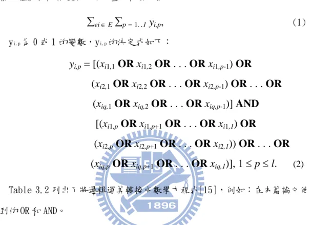
Table 3.1 列出了在 ILP 公式中所有變數所代表的意義以及變數的限制。而 目標方程式為計算 TSV 的使用量，計算方式如下：





y

,

yi,p為 0 或 1 的變數，yi,p的決定式如下：

y

= [(x

OR x

OR . . . OR x

) OR

(x

OR x

OR . . . OR x

) OR . . . OR

(x

OR x

OR . . . OR x

)] AND

[(x

OR x

OR . . . OR x

) OR

(x

OR x

OR . . . OR x

)) OR . . . OR

(x

OR x

OR . . . OR x

)], 1



p



l.

Table 3.2 列出了將邏輯運算轉換成數學方程式[15]，例如：在本篇論文使 用到的 OR 和 AND。

結合 Table 3.1 和 Table3.2 可以完整得到我們 ILP 的公式，而從變數可得 知，我們可以任意地調整變數的限制或面積平衡系數，在這方面有很大的彈性空 間。

14

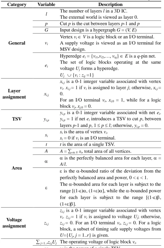
Table 3.1 Variables used in our generic ILP formulation.

Category Variable Description

General

l The number of layers l in a 3D IC.

The external world is viewed as layer 0.

p Cut p is the cut between layers p-1 and p

G Input design is a hypergraph G = (V, E)

vi Vertex vi V is a logic block or an I/O terminal. ei

Hyperedge ei = {vi1,vi2,…, viq}  E is a q-pin

net.

Layer

assignment xi,j

xi,j is a 0-1 integer variable associated with

vertex vi. xi,j = 1 if vi is assigned to layer j;

otherwise, xi,j = 0.

For an I/O terminal vi, xi,0 = 1, while for a logic

block vj, xj,0 = 0.

TSV yi,p

yi,p is a 0-1 integer variable associated with net ei. yi,p = 1 if net ei introduces a TSV to cut p,

between layers p-1 and p, 1  p  l; otherwise,

yi,p = 0.

Area

si

si is the area of vertex vi. si = 0 if vi is an I/O terminal.

t t is the area of a single TSV.

A A = viV si, total area of all vertices.

  is the perfectly balanced area for each layer, 

= A/l.



 is the -bounded ratio of the deviation from the perfectly balanced area, 0 <  < 1.

The -bounded area for each layer is subject to the range [(1-), (1+)].

Table 3.2 Logical expressions vs. mathematical constraints [16].

Logical Expression Mathematical Constraints

C = A AND B C  A C  B C A+B-1 C = A OR B C  A C  B C  A+B

15

3.4

ILP Reduction

3.4.1

Iterative ILP

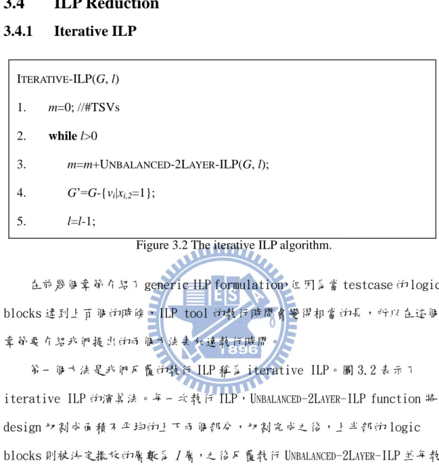
在前幾個章節介紹了 generic ILP formulation，但因為當 testcase 的 logic blocks 達到上百個的時候，ILP tool 的執行時間會變得相當的長，所以在這個 章節要介紹我們提出的兩個方法去加速執行時間。

第一個方法是我們反覆的執行 ILP 稱為 iterative ILP。圖 3.2 表示了 iterative ILP 的演算法。每一次執行 ILP，UNBALANCED-2LAYER-ILP function 將

design 切割成面積不平均的上下兩個部分，切割完成之後，上半部的 logic blocks 則被決定擺放的層數為l 層，之後反覆執行 UNBALANCED-2LAYER-ILP 並每執

行一次則將l – 1 直到完成 3D IC 的結構。特別的一點是當l 為 1 的時候，代

表所剩下的 logic blocks 已經不用再被切割，直接擺放至第一層。 Figure 3.2 The iterative ILP algorithm.

ITERATIVE-ILP(G, l)

1. m=0; //#TSVs 2. while l>0

3. m=m+UNBALANCED-2LAYER-ILP(G, l);

4. G’=G-{vi|xi,2=1};

16

UNBALANCED-2LAYER-ILP function 基本上與章節 3.3 所介紹的 generic ILP

formulation 大致相同，除了在面積的限制式上。因為 UNBALANCED-2LAYER-ILP

function 是將 design 切割成面積不平均的兩個部分，所以我們是對切割出來的 上半部分去做限制，而稍做更改的 formulation 如下：

3.4.2

Pre-clustering

第二個方法是我們在執行 ILP 之前先將 design 作 pre-clustering 的步驟。 我們參考[19]所提出的方法去減少 ILP 所需處理的變數量，將 logic blocks 降 低為 100 個之內。我們將連結性較強的幾個 logic blocks 綁在一起，例如：pin 點為 3 個以上的 net，我們先將這條 net 所連接的 logic blocks 綁在一起成為 一個新的 subset，之後對於剩下的 logic blocks，再從其中挑選較小的λ值。 λ值代表的是對外連結性的強弱，一個 logic block 的λ值算法為假若它在這個 新的 subset 之中，它所連接且不在這個 subset 之中的 pin 點有幾個。

minimize eiEp=1,2 yi,p

subject to j=0..2 xi,j = 1, viV;

17

Chapter 4

An Extension to MSV Design

基於 ILP 的彈性，我們將 chap 3.3 所提出的 ILP 公式擴展到考慮 MSV。每 一個 logic block 會有多個工作電壓可作選擇，所以在這個章節我們將 power 的 限制式加入到原始的 ILP 中。

4.1

Problem Definition

因為多考慮了 MSV 的情況，ILP 解答的目標改變為盡量降低 TSV 的使用量、 投影面積以及功耗。因此，多考慮 MSV 的 ILP 問題定義如下：

Problem: l-layer 3D IC Partitioning with MSV

給予一個整數 l 層的 3D IC 和一個電路設計包含了 logic blocks、I/O terminal 和它們彼此之間的相連關係(nets)，還有每個 logic block 可以選擇的 供應工作電壓，結果要找到切割好為 l 層的子電路，並且要做到盡量使 TSV 的數量最少，三維積體電路各層的面積盡量皆平均和盡量減少總功耗。

18

4.2

Extended ILP Formulation for MSV Design

Table 4.1 列出了在考慮 MSV 的情況下，所有變數所代表的意義以及變數的 限制。和 Table 3.1 並不考慮 MSV 的情況下的所有變數和限制式去做比較，Table 4.1 更多加了關於控制電壓的變數和 power 的限制式。值得注意的一點是，在最 後計算總電源的時候，並不是只有考慮 logic blocks 更要包含考慮 TSV 的電源。 而當一個 supply voltage 有被選擇使用時，我們就會把它建構為一個 I/O terminal，選擇使用這個 supply voltage 的 logic blocks 會連接它，以 voltage level 來看，形同一條 net。

19

Table 4.1 Variables used in our extended ILP formulation for MSV design.

Category Variable Description

General

l The number of layers l in a 3D IC.

The external world is viewed as layer 0.

p Cut p is the cut between layers p-1 and p

G Input design is a hypergraph G = (V, E)

vi

Vertex vi  V is a logic block or an I/O terminal. A supply voltage is viewed as an I/O terminal for MSV design.

ei

Hyperedge ei = {vi1,vi2,…, viq}  E is a q-pin net. The set of logic blocks operating at the same voltage Uj forms a hyperedge.

Uj  {vi : zij =1}

Layer

assignment xi,j

xi,j is a 0-1 integer variable associated with vertex

vi. xi,j = 1 if vi is assigned to layer j; otherwise, xi,j = 0.

For an I/O terminal vi, xi,0 = 1, while for a logic block vj, xj,0 = 0.

TSV yi,p

yi,p is a 0-1 integer variable associated with net ei.

yi,p = 1 if net ei introduces a TSV to cut p, between layers p-1 and p, 1  p  l; otherwise, yi,p = 0.

Area

si

si is the area of vertex vi.

si = 0 if vi is an I/O terminal.

t t is the area of a single TSV.

A A = viV si, total area of all vertices.

  is the perfectly balanced area for each layer,  =

A/l.



 is the -bounded ratio of the deviation from the perfectly balanced area and power, 0 <  < 1. The -bounded area for each layer is subject to the range [(1-), (1+)], while the -bounded power for each layer is subject to the range [(1-), (1+)].

Voltage

assignment zi,j

zi,j is a 0-1 integer variable associated with vertex

vi. zi,j = 1 if vi is assigned to voltage Uj; otherwise,

zi,j = 0. For an I/O terminal vi, zi,j = 0. For a logic block, a subset of timing safe supply voltages from

U={Uj, j = 1..r} is given.

Power

 j=1..rzi,jUj The operating voltage of logic block vi.

w w is the power of a single TSV. P P = viV si(k=1..r zi,kUk 2 ) + weiEp=1..l yi,p, total power. Pj Pj = viV sixi,j(k=1..r zi,kUk 2 ) + weiE yi,j, total power for layer j. For simplicity, the TSV power for cut j is included at layer j.

  is the perfectly balanced logic power for each

20

4.3

Speed-up

經過了考慮 MSV 的情況，我們依然可以使用 iterative ILP 去加速，對 chap 3.4 的 ILP 公式更多加了關於 power 的限制式，其方程式更改如下：

minimize eiEp=1,2 yi,p

subject to j=0..2 xi,j = 1, j=1..r zi,j = 1,viV;

(1-)viV si xi,j + teiE yi,j (1+), j=2,

21

Chapter 5

Experimental Results

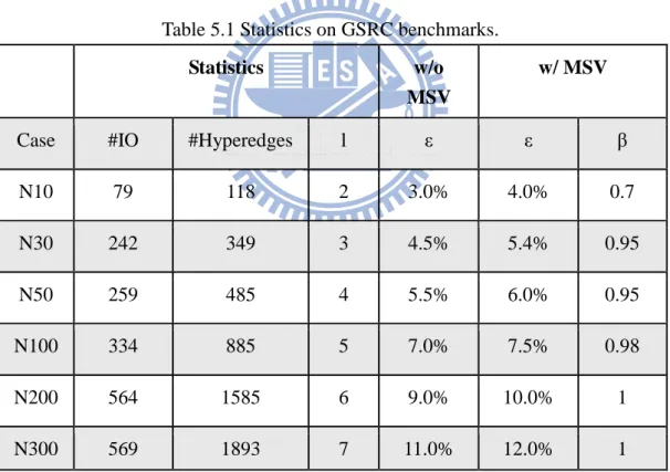
本篇論文之演算法以 C++程式語言並結合 IBM ILOG CPLEX 實現[18]。 以下將呈現 6 個 GSRC floorplanning benchmarks 執行的數據。Table 5.1 的左半部列出每個 benchmark 的 IO 數目、hyperedges 數目及所切割的層數。Table 5.1 的右半部是每個 benchmark 在不考慮 MSV 和考慮 MSV 的情況下，所設定的各 層面積係數和總電源係數。

Table 5.1 Statistics on GSRC benchmarks.

Statistics w/o

MSV

w/ MSV

Case #IO #Hyperedges l ε ε β

N10 79 118 2 3.0% 4.0% 0.7 N30 242 349 3 4.5% 5.4% 0.95 N50 259 485 4 5.5% 6.0% 0.95 N100 334 885 5 7.0% 7.5% 0.98 N200 564 1585 6 9.0% 10.0% 1 N300 569 1893 7 11.0% 12.0% 1

22

5.1

Generic ILP vs. Iterative ILP

Table 5.2 列出了 generic ILP 與 iterative ILP 的實驗結果。前 3 欄列出 了每個 testcase 的基本資訊；第 4 和第 5 欄分別是每個 testcase 所要切割出來 的層數和每層面積平衡的係數；第 6、第 7 欄為 generic ILP 所算出來的 TSV 數 量和執行所需時間；8、9 欄為 iterative ILP 初始沒有經過 pre-clustering 步 驟所算出來的 TSV 數量和執行所需的時間；最後兩欄為 iterative ILP 但初始經 過 pre-clustering 步驟所算出來的 TSV 數量和執行所需的時間。

從實驗結果可以得知，iterative ILP 改善了 generic ILP 的執行時間，平 均加速了 71 倍，甚至是最小的 case，n10，也可以加速到 2 倍快。第二，儘管 我們加快了 generic ILP 的執行時間，但在 iterative ILP 中使用 TSV 的數量不 超過在 generic ILP 中 TSV 數量的 5％。換句話說，iterative ILP 保留了 generic ILP 的最佳化。平均來說，從前三個 testcase 可以看到，我們的 iterative ILP 加快了 71 倍，而 TSV 數量卻只多了 4.3％。對於較大的 testcase 情況下，n200 和 n300，iterative ILP 和 pre-clustering 結果表現出，經過了 pre-clustering 的步驟更可以加快 iterative ILP，到達幾乎 2 倍的加速。

23

Table 5.2 Results on GSRC benchmarks with single voltage.

*: NA represents the ILP formulation is terminated by CPLEX. **

: The average of the first three cases

testcase #vertices #hyperegdes l  (%)

Generic ILP Iterative ILP

w/o pre-clustering w/ pre-clustering #TSVs runtime (sec) #TSVs runtime (sec) #TSVs runtime (sec) n10 79 118 2 3.0 115 0.18 124 0.09 n30 242 349 3 4.5 481 38.13 517 4.44 n50 259 485 4 5.5 715 3610.86 726 45.69 n100 434 885 5 7.0 NA* NA* 1204 124.19 1295 28.735 n200 764 1585 6 9.0 NA* NA* 2536 11592.00 3015 5550.47 n300 869 1893 7 11.0 NA* NA* 3288 21645.90 4153 11153.10 Average -- -- -- -- _1.000** 1.000** 1.043** 0.014** -- --

24

5.2

ILP with MSV

Table 5.3 列出了 generic ILP 與 iterative ILP 分別考慮 MSV 的實驗結 果。前 3 欄列出了每個 testcase 的基本資訊；第 4 和第 5 欄分別是每個 testcase 所要切割出來的層數和每層面積平衡的係數；第 6、第 7 欄為 generic ILP 所 算出來的 TSV 數量和執行所需時間；8、9 欄為 iterative ILP 初始沒有經過 pre-clustering 步驟所算出來的 TSV 數量和執行所需的時間；最後兩欄為 iterative ILP 但初始經過 pre-clustering 步驟所算出來的 TSV 數量和執行所 需的時間。

從實驗結果可以得知，iterative ILP 達到了加速 142 倍並且比起 generic ILP 幾乎沒有使用多餘的 TSV。我們更可以看到 n50 的 iterative ILP 達到了 92 倍速，同時節省 6％TSV 的數量。這種情況表明，TSV 的數量其實可以忽略不 計。同樣的，在較大的 testcase 情況下，n200 和 n300，經過了 pre-clustering 的步驟更可以加快 iterative ILP，到達幾乎 2 倍的加速。

25

Table 5.3 Results on GSRC benchmark with MSV.

*

: NA represents the ILP formulation is terminated by CPLEX. **

: The average of the first three cases.

testcase #vertices #hyperegdes l  (%)

Generic ILP Iterative ILP

w/o pre-clustering w/ pre-clustering #TSVs runtime (sec) #TSVs runtime (sec) #TSVs runtime (sec) n10 79 118 2 4.0 118 3.85 127 5.23 n30 242 349 3 5.4 484 3616.67 518 11.13 n50 259 485 4 6.0 799 3611.67 749 39.30 n100 434 885 5 7.5 NA* NA* 1229 192.11 1322 62.453 n200 764 1585 6 10.0 NA* NA* 2761 11985.30 3180 5863.11 n300 869 1893 7 12.0 NA* NA* 3321 21620.30 4196 10804.70 Average -- -- -- -- 1.000** 1.000** 0.988** 0.007** -- --

26 圖 5.1 比較了 iterative ILP 考慮 MSV 與不考慮 MSV 的兩種情況下，TSV 的 數量（見圖 5.1（a））和執行時間（見圖 5.1（b））。隨著多了 MSV 的情況下，有 多少 TSV 被使用於提供不同的電壓必須加以考慮。因此，TSV 數量自然是考慮了 MSV 的 iterativeILP 較不考慮 MSV 要來的多。實驗結果表示，考慮了 MSV 多了 將近 6％以上的 TSV 數量。圖 5.1（b）展示了兩個 ILPs 的執行時間。因為多了 關於電壓的變數與限制式，ILP 的複雜性增加，導致收斂速度較慢。考慮 MSV 的 iterative ILP 執行時間多花費了將近 2％。然而， iterative ILP 的執行時間 是數百倍快於 generic ILP，所以，考慮與不考慮 MSV 之間執行時間的差異是可 以容忍的。

圖 5.2 和圖 5.3 比較了 iterative ILP 是否經過 pre-clustering 步驟與不 經過 pre-clustering 步驟的兩種情況下，TSV 的數量和執行時間。實驗結果表 示，不論是否考慮 MSV，經過 pre-clustering 多了將近 2 成的 TSV 數量。然而， 因為減少了 ILP 的資訊處理量，使得執行時間縮短了一倍以上的時間。

27

(a)

(b)

28

(a)

(b)

Figure 5.2 Comparisons of (a) #TSVs and (b) runtime between iterative ILP w/ pre-clustering and w/o pre-clustering.

29

(a)

(b)

Figure 5.3 Comparisons of (a) #TSVs and (b) runtime between iterative ILP with MSV w/ pre-clustering and w/o pre-clustering.

30

Chapter 6

Conclusion

6.1

Concluding Remarks

31

Bibliography

[1] W. R. Davis, J. Wilson, S. Mick, J. Xu, H. Hua, C. Mineo, A. M. Sule, M. Steer, and P. D. Franzon, “Demystifying 3D ICs: The Pros and Cons of Going Vertical,”

IEEE Design & Test Magazine, pp. 498–510, Nov.-Dec., 2005.

[2] W.-L. Hung, G. Link, Yuan Xie, N. Vijaykrishnan, and M. J. Irwin, "Interconnect and Thermal-aware Floorplanning for 3D Microprocessors." in Proc ISQED, pp. 98–104, Mar. 2006.

[3] C. Ferri, S. Reda, and R. I. Bahar, “Parametric Yield Management for 3D ICs: Models and Strategies for Improvement,” ACM Journal on Emerging

Technologies in Computing Systems, 4(4), pp. 19:1–19:22, 2008.

[4] X. Dong and Y. Xie, “System-Level Cost Analysis and Design Exploration for Three-Dimensional Integrated Circuits,” in Proc. ASP-DAC, pp. 234–241, 2009. [5] The International Technology Roadmap for Semiconductors (ITRS), 2008.

Available: http://www.itrs.net/.

[6] Z. Yi, X. Hong, Q. Zhou, Y. Cai, J. Bian, H. Yang, P. Saxena, and V. Pitchumani, “A Divide-and-Conquer 2.5-D Floorplanning Algorithm based on Statistical Wirelength Estimation,” in Proc. ISCAS, pp. 6230–6233, 2005.

[7] T. Yan, Q. Dong, Y. Takashima, and Y. Kajitani, “How Does Partitioning Matter for 3D Floorplanning?” in Proc. GLSVLSI, pp. 73–78, Apr. 2006.

[8] G. Karypis, R. Aggarwal, V. Kumar, and S. Shekhar, “Multilevel Hypergraph Partitioning: Application in VLSI Domain,” IEEE Trans on Very Large Scale

32

[9] D. M. Kwai, “Homogeneous integration for 3D IC with TSV,” in Proc. ASP-DAC, pp. 546–547, 2010.

[10] H. S. Ye, M. C. Chi, and S. H. Huang, “A design partitioning algorithm for Three Dimensional Integrated Circuits,” IEEE International Symposium on Computer, Communication, Control and Automation (3CA) , pp. 229-232, 2010. [11] Y. C. Hu, Y. L. Chung, and M. C. Chi, “A multilevel multilayer partitioning

algorithm for three dimensional integrated circuits,” in Proc ISQED, pp. 483–487, 2010.

[12] S. Lee, K. Kang, and C. M. Kyung, “Temperature- and bus traffic- aware data placement in 3D-stacked cache,” in Proc. VLSI-SoC, pp.352–357, 2010.

[13] B. Noia, S. K. Goel, K. Chakrabarty, E.J. Marinissen, and J. Verbree,

“Test-architecture optimization for TSV-based 3D stacked ICs,” in Proc. ETS, pp.24–29, 2010.

[14] C. M. Fiduccia and R. M. Mattheyses, “A Linear-Time Heuristic for Improving Network Partitions,” in Proc. DAC, pp. 175–181, 1982.

[15] L. Schrage, Optimization Modeling with LINGO, 6th ed., Lindo Systems Inc., 2008.

[16] GSRC benchmark.

[17] I. H. R. Jiang, “Generic Integer Linear Programming Formulation for 3D IC Partitioning,” in Proc. SOCC, pp. 321–324, 2009.

[18] IBM ILOG CPLEX Optimizer. Available:

33

[19] T. Jindal, C. J. Alpert, J. HU, Z. Li, G.-J. Nam and C. B. Winn, “Detecting Tangled Logic Structures in VLSI Netlists,” in Proc. DAC, pp. 603–608, 2010.