最大化存貨投資報酬的中盤商退化性商品存貨模式

行政院國家科學委員會專題研究計畫 成果報告

最大化存貨投資報酬的中盤商退化性商品存貨模式 研究成果報告(精簡版)

計 畫 類 別 ： 個別型

計 畫 編 號 ： NSC 97-2410-H-011-006-

執 行 期 間 ： 97 年 08 月 01 日至 98 年 07 月 31 日 執 行 單 位 ： 國立臺灣科技大學資訊管理系

計 畫 主 持 人 ： 陳正綱

處 理 方 式 ： 本計畫可公開查詢

中 華 民 國 98 年 12 月 28 日

行政院國家科學委員會補助專題研究計畫 ■ 成 果 報 告

□期中進度報告

（計畫名稱）

最大化存貨投資報酬的中盤商退化性商品存貨模式

A Deteriorating Inventory Model for Intermediary Firms under Return on Inventory Investment Maximization

計畫類別：■ 個別型計畫 □ 整合型計畫 計畫編號：NSC 97-2410-H-011-006

執行期間： 97 年 8 月 1 日至 98 年 7 月 31 日

計畫主持人：陳正綱 共同主持人：

計畫參與人員：廖益祥、林駿甫

成果報告類型(依經費核定清單規定繳交)：■精簡報告 □完整報告

本成果報告包括以下應繳交之附件：

□赴國外出差或研習心得報告一份

□赴大陸地區出差或研習心得報告一份

□出席國際學術會議心得報告及發表之論文各一份

□國際合作研究計畫國外研究報告書一份

處理方式：除產學合作研究計畫、提升產業技術及人才培育研究計畫、

列管計畫及下列情形者外，得立即公開查詢

□涉及專利或其他智慧財產權，□一年□二年後可公開查詢

執行單位：國立台灣科技大學 資訊管理學系

中 華 民 國 九十八 年 十二 月 二十八 日

行政院國家科學委員會專題研究計畫成果報告

最大化存貨投資報酬的中盤商退化性商品存貨模式

A Deteriorating Inventory Model for Intermediary Firms under Return on Inventory Investment Maximization

計畫編號：NSC 97-2410-H-011-006 執行期限：97 年 8 月 1 日至 98 年 7 月 31 日

主持人：陳正綱 執行機構及單位名稱：國立台灣科技大學資訊管理學系 計畫參與人員：廖益祥、林駿甫

中文摘要

本研究計劃的目的，是從中盤商的角 度以最大化存貨投資報酬為目標，來考慮 具退化性質的產品時之最佳採購週期。首 先，將透過數學模式的建立與分析來推導 在下最佳採購週期的特性。根據這些推導 出來的特性，我們將發展有效率的求解演 算法來求得模式最佳解以提供決策者最佳 採購週期決策的參考

在存貨系統中，就進、補貨或採購週 期的決策，本研究計劃的重要性在於拓展 原本對該領域的認識。不僅以中盤商為決 策者來最大化其存貨投資報酬，同時也將 考慮具退化性質的產品對決策的影響，來 提供決策者最佳進、補貨與採購週期的決 策的參考。

關鍵詞：：存貨、中盤商、存貨投資報酬 最大化、退化性產品。

Abstract

The objective of this project is to explore the deteriorating products for the intermediary firms to determine the optimal purchasing cycle under return on inventory investment maximization (ROII maximi- zation). Through the formulation and analyses of the mathematical model, several interesting and useful properties will be derived. By fully utilizing these properties, an efficient search algorithm will be developed. From the development of our models and the results of this project, several decision- making rules, managerial insights, and economic implications are expected to be obtained.

Keywords: Inventory, Intermediary Firm, ROII maximization, Deteriorating Product

1. Introduction

In a supply chain logistics system, the function of an intermediary firm is to purchase products and to sell those purchased products to the public or to other firms.

(see e.g., Chen and Min [1]). This paper investigates how the intermediary firms can optimally determine the purchasing cycle length of a deteriorating product under return on inventory investment (ROII) maximization. By incorporating the deteriorating nature of products and the special structure of the intermediary firm’s environments into the traditional economic order quantity (EOQ) model, we mathematically formulate the inventory problem encountered by the intermediary firms as a ROII maximization problem.

Several interesting properties of the optimal policy are investigated and an efficient algorithm is provided to search for the optimal solution.

In practice, the intermediate firms described in this paper can be easily found in numerous industries. For example, the personal computer assembly firms purchase electronic components from independent producers. Also, Chen and Min [1] presents two examples of intermediate firms in the agricultural industry as well as the garment and apparel industry. For the mathematical formulation of the inventory problem for intermediary firms, Chen and Min [1] first investigated how intermediary firms can optimally determine both the selling quantity and the purchasing price of a product. Chen [2] extended Chen and Min [1] to propose a profit maximization inventory model to optimally determine the quality level, the

selling quantity and the purchasing price of a product for the intermediary firms.

Traditionally, cost minimization (or profit maximization) is widely utilized as the performance measure of inventory models (see e.g., Silver et al. [3], Smith [4], or Ladany and Sternlieb [5]). In Schroeder and Krishnan [6], an inventory model is proposed under an alternative performance measure of return on investment (ROI) maximization. Rosenberg [7] considers the logarithmic concave demand functions and examines the inventory models under profit maximization vs. return on inventory investment maximization. More recently, Toshitsugu et al. [8] constructs and analyzes inventory and investment in setup operations policies under return on investment maximization. We note that the last three ROII-related papers deal with the inventory models from the perspectives of a retailer or a producer. In contrast to the perspectives of a retailer or a producer, the proposed inventory model in this paper is constructed and analyzed from the perspectives of an intermediate firm. In addition, the deterioration nature of products is considered in this paper.

The literature concerning the deterioration nature of the product from the perspectives of a retailer or a producer instead of from the perspectives of an intermediary firms is well documented.

Ghare and Schrader [9] first proposed an EOQ model with an exponentially deteriorating inventory. More recently, numerous research works (see e.g., Padmanabhan and Vrat [10], Sarker et al.

[11], Giri and Chaudhuri [12], Chung, Chu and Lan [13], Jalan and Chaudhuri [14], Wee and Law [15] and Dye and Ouyang [16]) ever discussed the deteriorating inventory models under different environmental scenarios and/or model assumptions.

Padmanabhan and Vrat [10] discussed three different EOQ models for deteriorating items under linearly stock dependent selling rate with no backlogging, complete backlogging and partial backlogging, respectively, and a comparison of these three models was given. Sarker et al. [11]

developed an order-level inventory model

with inventory-level dependent demand and deterioration by relaxing infinite production rate in the model shown in Padmanabhan and Vrat [10]. Giri and Chaudhuri [12]

proposed two EOQ models for a perishable product with stock-dependent demand rate and with / without nonlinear holding cost.

Chung, Chu and Lan [13] extended Padmanabhan and Vrat’s [10] work, and showed the necessary and sufficient conditions for the existence and uniqueness of the Padmanabhan and Vrat’s [10] no backlogging and complete backlogging inventory models. We note that the intersection of the above four papers lies on the inventory (or stock) – dependent demand for the deteriorating inventory problem.

Jalan and Chaudhuri [14] developed an inventory model for a deteriorating item under linearly time dependent demand rate with a linearly positive trend, and provided some properties of the model. Wee and Law [15] proposed an EPQ model for Weibull deteriorating items taking the time-value of sale revenues, set-up cost, inventory cost, shortage cost and item cost into consideration and found that when Weibull deterioration conforms to exponential deterioration, the production run time will be shorter. Dye and Ouyang [16]

extended the model shown in Padmanabhan and Vrat [10] by introducing a time-proportional backlogging rate. We note that the above three papers emphasized the importance of “time” factor on the deteriorating inventory models.

However, there has been few literatures concerning the deteriorating nature of the product from the perspective of the intermediary firm. In this paper, we attempt to incorporate the deterioration nature of the product into a ROII maximization model to determine the optimal purchasing cycle length for the intermediary firm. The rest of this paper is organized as follows. We first describe the model environments of the proposed problem for the intermediary firm.

Then, we mathematically formulate the proposed problem as a ROII maximization model. From the mathematical formulation, we derive three interesting properties to carry out an efficient algorithm to search for the

optimal purchasing cycle length for the intermediary firm. At the very last, a numerical example is provided and the concluding remarks are made.

2. Description of the model environments

The unit price that an intermediary firm pays to independent producers is denoted by

r for a single type of deteriorating products

(e.g., fruits or milk). The supply rate of the deteriorating product to the intermediary firm from the independent producers at price

r

is given by

s r . We note that a higher

( ) price r implies a higher supply rate ( )

s r ,

i.e.,

( ) 0

s r

r

∂ >

∂ . The purchased products of the intermediary firm from independent producers are assumed to be exponentially deteriorated with deterioration rate θ . Therefore, the rate of change of inventory level can be expressed as the following linear first order differential equation

t ( )

t

dI I s r dt

+

θ

=

(1) where

I

^t

represents the inventory level at time t . Additionally, the boundary condition of the differential equation (1) is that

I

⁰ =0

. By employing integrating factor and the boundary condition

I

⁰ =0

, the solution of differential equation (1) is

( )( ^t 1)

t t

s r e

I e

θ

θ

θ

= −

(2) where

^{t ∈}

[ ]

^{0, T}

and

( )( ^T 1)

T T

s r e

I e

θ

θ

θ

= −

(3) Here, T represents the time length between two successive selling points of the purchased products of the intermediary firm.

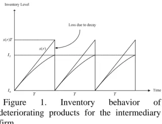
The graphical representation of the inventory behavior can be shown as in Figure 1. The purchased products of the intermediary firm are continuously checked to see if deterioration occurs or not. If the purchased units deteriorate, then dispose them

immediately. The non-deteriorating purchased products are stored in the warehouse of the intermediary firm at a cost of rF per unit per unit time where F is the per unit time holding cost as a fraction of the unit purchasing cost to the intermediary firm. Once an amount of non-deteriorating

I

T

units accumulates, all of the non-deteriorating

I

^T

units are sold to another firm that further processes or utilizes the products (or sell them to the public) at a given price of p per unit. We note that the given price p which is the intermediate firm sells the purchased products to another firm or to the public is greater than the unit price r that an intermediate firm pays to numerous independent producers. Namely,

p

>

r

is assumed. The cost incurred by the intermediary firm in selling the accumulated non-deteriorating products is represented by a fixed selling cost K and a variable selling cost

^c

per unit.

T T T

IT

I0

( ) s r ( )

s r T

Figure 1. Inventory behavior of deteriorating products for the intermediary firm

3. Mathematical Formulation for the Intermediary Firm

Under our definitions, assumptions and environment description, the revenue per cycle for the intermediary firm is given by

pI

T

while the payment to the independent producers per cycle is given by

rs r T .

( ) The total selling cost per cycle is

K

+

cI

^T

. The inventory holding cost per cycle is expressed as

0 0

2

( )( 1) ( ) 1

T T t

t t

T T

T

s r e

rF I dt rF dt

e Te e rFs r

e

θ θ

θ θ

θ

θ θ

θ

= − =

⎛ + − ⎞

⎜ ⎟

⎝ ⎠

∫ ∫

(4) Therefore, the profit per cycle,

PRPC T ,

( ) which is the revenue less the cost, is given by

0

( )

_T

( )

T

T t

PRPC T pI rs r T K cI rF I dt

= − −

− − ∫

(5) By substituting equations (2), (3), (4) into equation (5), we can have the following expression for

PRPC T :

( )

( )

( )

2

( ) 1

( ) ( )

( ) 1

T

T

T T

T

p c s r e

PRPC T rs r T

e

Te e K rFs r

e

θ

θ

θ θ

θ

θ

θ θ

− −

= −

⎛ + − ⎞

− − ⎜ ⎟

⎝ ⎠ (6)

In practice, no firm is willing to operate with negative profit in the long run. Therefore, in this paper, we assume that the profit level for the intermediary firm is non-negative.

The corresponding total profit per unit time,

PRPUT T , can be obtained by dividing

( )

( )

PRPC T

by T , the cycle length.

Namely,

( )

( )

2

( ) 1

( ) ( )

( ) 1

T

T

T T

T

p c s r e

PRPUT T rs r

Te

K rFs r Te e

T T e

θ θ

θ θ

θ

θ θ

θ

− −

= −

⎛ + − ⎞

− − ⎜ ⎟

⎝ ⎠

(7)

And the average inventory investment should be

0 0

2

( )( 1) ( )

( ) 1

T T t

t t

T T

T

r r s r e

AII T I dt dt

T T e

Te e

rs r Te

θ θ

θ θ

θ

θ θ

θ

= = −

⎛ + − ⎞

= ⎜ ⎟

⎝ ⎠

∫ ∫

(8)

Therefore, the return on inventory investment is given by dividing

PRPUT T

( ) by

AII T (see e.g., Schroeder and Krishnan

( ) [6], Rosenberg [7], and Tshiitsugu et al. [8]).

Namely,

( )

( )

( )

( )

2

2

( ) 1 1

1

( ) 1

T

T T

T

T T

T

T T

p c e ROII T

r Te e

Te Te e

K e

F

rs r Te e

θ

θ θ

θ

θ θ

θ

θ θ

θ θ θ θ

θ θ

− −

= + −

− + −

− −

+ −

(9)

In order to obtain the return on inventory investment maximizing cycle time length

T ,

^*

ROII T is differentiated with respect to T

( ) and set equal to zero. Hence,

( )

( )

( )

( )

( )

( )

( )

( )

( )

2

2

3

2

2

2

( )

1 1

1 ( ) 1

( ) 1 1

( ) 1 0

T T

T T

T T

T T

T T

T

T T

ROII T T

p c r e T e

r Te e

K e e

rs r Te e

p c r s r T e e

K e

rs r Te e

θ θ

θ θ

θ θ

θ θ

θ θ

θ

θ θ

θ θ

θ θ

θ θ θ

θ θ

∂ =

∂

− − + −

+ −

− −

+ −

⎡ − − + − ⎤

⎢ ⎥

⎢ − − ⎥

⎣ ⎦

= + −

=

(10)

We note that it is very difficult to find the optimal closed-form solution

T

^* from equation (10). Instead, several interesting properties are derived for the proposed problem so that the optimal solution

T can

^* be obtained.

4. Solution Procedure for the PRPUT Maximization Model

In this section, the uniqueness property of the optimal cycle length

T is obtained

^* and an approximate solution is derived.

Specifically, the approximate solution provides upper bound for searching the optimal cycle length

T .

^*

Proposition 1. If ROII T is given by

( ) equation (9), then there exists an unique optimal

T

^*> maximizing 0

ROII T .

( ) Proof: Please see appendix A.

Although Proposition 1 shows that an

optimal cycle length exists and is unique,

T

^* can only be obtained by a nonlinear search procedure since there is no closed form expression for

T . However, when the

^* when the deterioration rate θ is small, we can obtain an approximate solution for optimal cycle length

T . The result is

^* summarized in the following proposition.

Proposition 2. If the deterioration rate θ is

small, then we can have an approximate

solution

^T

^a*

⁼

(

^{p − − c r s r 2}

)

^{K ( ) − K}

^θ _.

Proof: Please see appendix B.

Although Proposition 2 shows that an approximate solution

*

T

a

can be obtained in closed form format, the relationship between

*

T

a

and

T

^* is still unknown. The following proposition clearly states the relationship between

*

T

a

and the optimal solution

T .

^*

Proposition 3. The approximate solution

*

T

a

is a upper bound of the optimal solution

T .

^* Proof: Please see appendix C.

Before presenting the iterative search procedure to find the optimal cycle length

T , we first rearrange equation (10) by some

*

algebraic manipulation and can obtain the following result.

( )

( )

2

1 ln 1 ,where

( )

T MT

M K

p c r s r K θ

θ θ

θ

= +

= +

− − −

(12)

Employing the existence and uniqueness properties in Proposition 1, the approximate solution for the cycle length in Proposition 2, the upper bound for the optimal cycle length in Proposition 3 and the equation (12), the iterative search procedure for the optimal cycle length

T can be facilitated and is

^* summarized as follows.

Step1:Compute

( )

(1) *

2

a

( ) T T K

p c r s r K θ

= =

− − −

Step 2: Set

^{i = 2}

, and compute

( )

( ) 1 ( 1)

ln 1

i i

T MT

θ

⁻

= +

Step 3: if

( )i (i1)

T

−

T

⁻ >

ε

, then go to Step 4.

Otherwise go to Step 5

Step 4: Set

^{i = + i 1}

and compute

T

^{( )i} , then go to Step 3.

Step 5: output

T

^{( )i} as the optimal cycle length

T , and calculate the corresponding

^*

ROII .

*

Although the above iterative search procedure can help us to find the optimal cycle length

T . However the sequence

^*

{ } ^T

^{( )i} may not converge to

T . In the

^* next proposition, we will show that the iterative search procedure we propose will converge to the unique optimal solution

T .

^*

Proposition 4. If the approximation solution

*

T

a

is chosen as the starting point of the iterative search procedure, the sequence

{ } ^T

^{( )i} will converge to the optimal solution

T .

*

Proof: Please see appendix D.

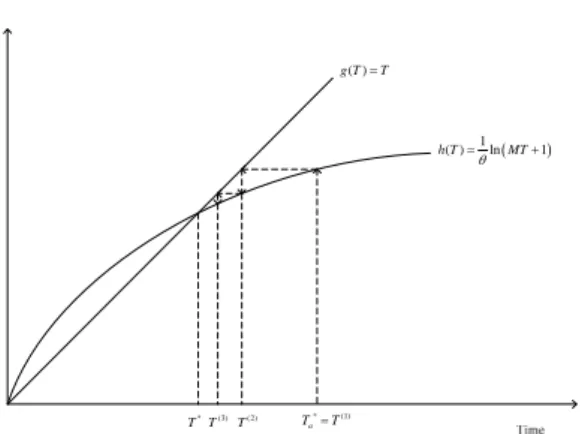
The iterative search procedure for the optimal cycle length

T can be depicted in

^* Figure 2. Let ( )

g T

=

T

represents the left hand side of equation (12) and

( )

( ) 1ln 1

h T MT

=

θ

+

represents the right hand side of equation (9). We note that the optimal cycle length

T occurs at the

^* intersection of ( )

g T and ( ) h T . Refer to

Figure 2, the optimal cycle length

T can

^* be found very efficiently.

* (1)

Ta=T T* T⁽²⁾

( ) g T=T

T(3)

( )

( ) 1ln 1

h T MT

=θ +

Figure 2. Iterative search procedure to find optimal cycle length

T .

^*

5. Numerical Example

In this section, we solve a ROII maximization problem over the cycle length

T to illustrate some of the features

discussed in this paper. First, we assume that the supply rate per unit time ( )

s r is a

linear function of r , the unit price that an intermediary firm pays to independent producers. That is, ( )

s r

=

gr

, where g is a positive proportionality constant. Let us assume that the following values are provided either by estimates from the free market or by regulatory rules.

5 K =

9

p

=

0.05 F =

0.5

g

=

0.5 c =

5 r =

θ

= 0.1

By employing the algorithm developed in the previous section, we can solve this numerical example very efficiently. Assuming

10 6

ε

= ⁻ , the outcome of each iteration is shown in Table 1.

Table 1. The outcome of each iteration to find optimal cycle length

T .

^*

From Table 1, we note that the optimal cycle length

T converges within three iterations.

^* Specifically, the optimal cycle length

T

^* and the corresponding return on inventory investment are given by 1.165508061719163 and 0.41628468277685, respectively. Next, we perform sensitivity analysis for the deterioration rate

θ

on the optimal cycle length

T and the corresponding

^*

ROII .

^*

6. Concluding Remarks

We have show how to formulate the return on inventory investment maximization problem for intermediary firms by incorporating the deteriorating nature of the purchased products. Three useful properties are derived to develop an efficient algorithm to search for the optimal cycle length. Also, the sensitivity analysis of the deterioration rate is presented.

There are several possible extensions of the proposed problem in this paper. For example, it would be interesting to examine the proposed problem under different performance measurement such as profit maximization or residual income. Another possible extension is to examine the interactions between independent producers (or supplier) and the intermediary from the perspective of game theory.

Iteratio n

( )i

T ROII

under

T

^{( )i}

1 1.212121 0.415413791764777 10 1.192797 0.415976286559608 30 1.173968 0.416254001455607 50 1.168151 0.416281631787386 70 1.166328 0.416284379518799 90 1.165755 0.416284652731335 110 1.165574 0.416284679896216 130 1.165517 0.416284682597105 138 1.165508 0.41628468277685

Appendix A

Proposition 1. If ROII T is given by

( ) equation (9), then there exists an unique optimal

T

^*> maximizing 0

ROII T .

( )

Proof: From equation (10), set ( ) 0

ROII T T

∂ =

∂ , we have

( )

( )

( )

( )

2

2

( ) 1

( ) 1

0 ( ) 1

T T

T

T T

p c r s r

e T e

K e

ROII T

T rs r Te e

θ θ

θ

θ θ

θ θ

θ θ

⎡ − − ⎤

⎢ ⎥

⎢ + − ⎥

⎢ ⎥

⎢− − ⎥

∂ = ⎣ ⎦ =

∂ + − (A.1)

Let ( )

( )

( )

( ) ( ) 1

1

T

T

f T p c r s r T e

K e

θ

θ

θ θ

= − − + −

− − (A.2)

To prove ( )

ROII T

0

T

∂ =

∂ has unique

solution, it is necessary to prove that ( ) 0

f T

= has unique solution.

It is clear that

0

lim ( ) 0

T ₊

f T

→ = . By

differentiating ( )

f T

with respect to T , then we have

( )

( )

2

( ) ( ) 1

^r

r

T

T

f T p c r s r e T

K e

θ θ

θ θ

∂ = − − −

∂ +

(A.3)

( )

2

2 2

( )

p c r s r

( ) _Tr

f T e

T K

θ

θ

θ

− −

⎡ ⎤

∂∂ = − ⎢⎣− ⎥⎦ (A.4)

If we can prove

f T is a concave function,

( ) and let

T

_f^* be the global maximum of

( )

f T

, then there exists a unique

T

^* in

( ^T

^f*,∞ such that

) f T

( ^*)= . 0

Since ROII cannot be negative, we have the following inequality.

( )

( ) ( )

( )

2

2

( ) 1 ( )

( ) 1 0

T T

T T T

p c s r e rs r Te

K e Frs r Te e

θ θ

θ θ θ

θ θ

θ θ

− − −

− − + − > (A.5)

Because 1+

θ Te

^θT −

e

^θT > , we can move 0 the fourth term of inequality of (A.5) to the right hand side of (A.5), then the following inequality holds

( )

( )

²

2

( ) 1 ( )

0

T T

T

p c s r e rs r Te

K e

θ θ

θ

θ θ

θ

− − −

− > (A.6)

By dividing θ on inequality (A.6), the following inequality holds

( ) ^{( )}

(

¹

)

^{( )}

0

T T

T

p c s r e rs r Te K e

θ θ

θ

θ θ

− − −

− > (A.7)

Since 1

e

^θT − <

θ Te

^θT , we can replace

T 1

e

^θ − in first term of (A.7) with

θ Te

^θT, then the following inequality holds

( ) ^{( ) ( )}

0

T T

T

p c s r Te rs r Te K e

θ θ

θ

θ θ

θ

− −

− > (A.8) By dividing

e

^θT on inequality (A.8), the following inequality holds

(

^{p − c s r}

)

^{( ) θ T − rs r ( ) θ T − K θ > 0}

(A.9) By pulling out the common term “θ ” of the

^T

first and second term, we have the following inequality

(

^{p − − c r s r}

)

^{( ) θ T − K θ > 0}

(A.10) We note that

θ T < 1

, hence we can replace θ in inequality (A.10) with 1 and the

T

following inequality holds

(

^p − − ^{c r s r}

)

^{( )} − ^K

θ

> ⁰

(A.11) With inequality (A.11) and (A.4), we can find that

2

2

( ) 0

f T

T

∂ <

∂ , and

f T

( ) is a concave function.

Thus

0

lim ( ) 0

T

f T K

T θ

→

∂ = >

∂ ,

2

2

( ) 0

f T

T

∂ <

∂ , and

*

T

f be the global maximum of

f T , it is

( ) clear

T

_f^*

> 0

, and it is not difficult to realize that ( )

f T is monotonic decreasing between

( ^T

^f*,∞ , then ( ) 0

) f T

= has unique solution between

( ^T

^f*,∞

)

, that is,

( ) 0

ROII T

T

∂ =

∂ has unique solution between

( ^T

^{f*,∞ .}

)

Let

T

^* be the unique solution of ( ) 0

ROII T T

∂ =

∂ , to prove

T

^* is the global maximum of

ROII T , it is necessary to

( ) prove that

2 *

2

( )

ROII T

0

T

∂ <

∂ .

By differentiate equation (10) and replace T with

T

^*, we have

( )

( )

* *

*

*

*

3

2 *

2

2 *

( ) 1

( )

( ) 1

T T

T

T

T

p c r s r

e e

ROII T K e

T T e

rs r e

θ θ

θ θ θ

θ

θ θ

⎡ − − ⎤

⎢ ⎥

⎢ − ⎥

⎢ ⎥

⎢ + ⎥

∂ = ⎣ ⎦

∂ ⎛ + ⎞

⎜ ⎟

⎜ − ⎟

⎝ ⎠

(A.11)

From (A.1), we can simplify (A.1) to

( )

( )

( )

( ) 1

1 0

T

T

p c r s r T e

K e

θ

θ

θ θ

− − + −

− − = (A.12) Rearrange (A.12), we have the following equation.

( )

( )

( )

^{( )}

( ) 1

1 0 ( )

T

T

p c r s r e

K e p c r s r T

θ

θ

θ

θ

− − − =

− − − − (A.13) Replace (

^{p − − c r s r}

)

^{( ) 1} ( ^{− e}

^θT*

)

in (A.11) with (A.13), we have the following equation.

( )

*

*

*

3

2 * *

2

2 *

( ) ( )

( ) 1

T

T

T

p c r e

s r T K ROII T

T T e

rs r e

θ

θ θ

θ θ θ

θ

⎡ − − ⎤

− ⎢ ⎥

∂ = ⎢⎣ − ⎥⎦

∂ ⎛ + ⎞

⎜ ⎟

⎜− ⎟

⎝ ⎠

(A.14)

From (A.10) and (A.14), we conclude that

T

* maximizing

ROII T

( ) globally has been proven.

Appendix B

Proposition 2. If the deterioration rate

θ is small, then we can have an approximate solution

( )

*

2

a

( ) T K

p c r s r K θ

= − − −

.

Proof: From equation (10),

T satisfies

^* ( *)

ROII T

0

T

∂ =

∂ , which can be simplified to (A.12). If the deterioration rate is small, by employing Taylor series expansion, we can have the following approximation.

( ) ( )

( ) ( )

2 3

4 2

1 2! 3!

...

4! 2!

T

T T

T e

T T

θ

θ θ

θ

θ θ

+ − = − −

− ≈ −

(A.15)

( ) ( ) ( )

2 3

2

1 2! 3!

...

2!

T

T T

e T

T T

θ

θ θ

θ θ θ

− = − − −

− ≈ − −

(A.16)

Substituting (A.15) and (A.16) into (A.12), (A.12) can be rewritten to

( )

( )

( )

* 2

* 2

*

( ) 2!

2! 0

a

a a

T p c r s r

K T T

θ

θ θ θ

⎡ ⎤

⎢ ⎥

− − − −

⎢ ⎥

⎣ ⎦

⎡ ⎤

⎢− − ⎥=

⎢ ⎥

⎣ ⎦

(A.17)

Therefore,

( )

*

2

a

( ) T K

p c r s r K θ

= − − −

(A.18)

Appendix C

Proposition 3. The approximate solution T

_a^* is a upper bound of the optimal solution

T .

^* Proof: It is not difficult to show that

2 2

1 1

2

e

T

T

T

θ

θ

θ

− − >

∀ > T 0

and

0 < < θ 1

Hence, we can let

* *

2 *2

1

2

e

T

T f

T

θ

θ

θ

− − = , where

f

> (A.19) 1 Since

T satisfies

^*

( )

( )

( )

* *

*

*

*

2 *

*

* 2

( ) 1

( ) 1

( ) 1

0

T T

T

T

T

p c r s r

e T e

K e

ROII T

T T e

rs r e

θ θ

θ

θ θ

θ θ

θ θ

⎡ − − ⎤

⎢ ⎥

⎢ + − ⎥

⎢ ⎥

⎢ ⎥

− −

⎢ ⎥

∂ = ⎣ ⎦

∂ ⎛ + ⎞

⎜ ⎟

⎜ − ⎟

⎝ ⎠

=

(A.20)

Rearrange (A.20), we have the following equation.

( )

( )

( )

( )

*

* *

*

*

4 *2

* 2

*

2 *2

2 *2

( ) 1

( ) 1

0 1

T

T T

T

T

T e

rs r T e e

p c r s r e T

T K e

T

θ

θ θ

θ

θ

θ θ

θ θ

θ θ

+ −

⎡ − − − − ⎤

⎢ ⎥

⎢ ⎥=

⎢ ⎥

⎢ − ⎥

⎢− ⎥

⎣ ⎦

(A.21)