暴漲宇宙的初始條件及其在宇宙背景輻射上所形成之特徵

(1)

國立臺灣大學理學院物理學系博士論文

Department of Physics College of Science

National Taiwan University Doctoral Dissertation

Initial Condition of the Inflationary Universe and Its Imprint on the Cosmic Microwave Background

林裕翔 Yu-Hsiang Lin

指導教授：陳丕燊博士 Advisor: Pisin Chen, Ph.D.

中華民國 106 年 6 月 June 2017

(2)

(3)

Acknowledgments

I want to thank Prof. Pisin Chen for bringing me into the field of physics research, giving me the environment and opportunity to fully dedicate myself into physics.

His support started from the time before I entered the physics department, all the way to the time I’m leaving. I also have my deepest gratitude to my mother and my father. You are very successful parents who help your son grow into a man who can face the challenges in life and pass them. I love you. To my partner and my guardian, the most beautiful Ting-An: Thank you for sharing the life with me.

I thank Prof. Jiunn-Wei Chen, Prof. Yu-tin Huang, Dr. Dong-han Yeom, and Dr. Frederico Arroja for being my thesis examination committee and their e↵ort.

I would also like to thank: Dr. Mariam Bouhmadi-L´opez and Yu-Chien Huang for giving me the opportunity to collaborate; Prof. Keisuke Izumi and Dr. Lance Labun for their support and many discussions, and being models of good researchers for me;

Dr. Frederico Arroja for his careful reading and thoughtful comments, from which I benefited a lot; Dr. Dong-han Yeom for working with me and his many interesting ideas; Prof. Teruaki Suyama, Prof. Pei-Ming Ho, Dr. Je-An Gu, Dr. Christo- pher Gauthier, Dr. Sean Downes, and Dr. Jinn-Ouk Gong, for their discussion and help; Prof. Jiwoo Nam for his teaching in physics and Korean; Prof. Tom Abel and Prof. Greg Madejski for having me at the KIPAC family in SLAC; Prof. Leonardo Senatore, Prof. Stephen Shenker, Prof. Eva Silverstein, and Prof. Andrei Linde for their discussion at SITP, Stanford University; Prof. Hitoshi Murayama, Prof. Ya- sunori Nomura, and Dr. Keisuke Harigaya for their help and discussion at Berkeley.

(4)

Special thanks go to all friends, faculties, and secretaries in LeCosPA, NTU, for helping me and supporting me all the time. The thesis and related works are in addition supported by Taiwan Ministry of Science and Technology, as well as Taiwan National Center for Theoretical Sciences.

It has been a precious and wonderful journey through the ocean of life for me.

Prof. Cha-Ray Chu once said, “Artistic creation is a constant progression. A creator must cherish her own work; even if it is not perfect, it is what she devoted herself to.” I am grateful for being lucky to have the opportunity of creating something, and being able to experience what she said. As American writer Elizabeth Gilbert put it, “you must stubbornly walk into that room, regardless, and you must hold your head high. You make it; you get to put it out there. Never apologize for it, never explain it away, never be ashamed of it. You did your best with what you knew, and you worked with what you had, in the time that you were given. You were invited, and you showed up, and you simply cannot do more than that.” The spirit of the Sand Hill Road days will always be a part of me.

(5)

X X XÅ Å Å

ûWMAP0Planck∫ [ Ñ¿,Pú- ⌘⌘ å↵0áôÆ‚Ão;⌅(w

‚w‚µÑ;\/ENº⇤CDM⇡ñáô!ãÑ⇣,⇥⇠°q ⌦⇡⇧ÓpÑ

À⇣UÕ⇡ñáô!ãÑzö'I⁄ ⌘⌘Õ6 7»Ñ’_ª⇤n¥2Máô

;\ë6ÑH…⇥¿,o:(¥2áô:¶®9 åÑe⁶⁰ ÊÛÑ ì·

¥24Ñ˝œ:¶∫10¹⁶↵A⌅˚P✏y⇥Çú(ÙÿÑ˝œ:¶· iÍUº

Ñ¯ ⇧Õõm0Óc G¥2MáôÑ~U Ô˝ º¥2B Ñ

—<sBzgÑde Sitteráô⇥( p}≥ Ñ¥2áô- ⌘⌘ Â@¿,

0Ñ':¶Æ˛È /(s⌥Å2e¥2B ÑN! D—‚ã»/®9ÑñL

0s⁄ ‡d⇡õ':¶Æ˛ãÊ⌦⌧6W¥2MáôÑ«⌦ ⌘⌘_Ô˝Ô

Âû':¶Ñ;\- ∫¥2MáôÑ ¯⇥

⌘⌘ñH⇤n ↵!ÆÑ⌃÷!ã⇥(⇡↵!ã- ¥2MáôEˇÜ1á¡

áô&⇡i.◊+”≤:w@À⇣Ñ≤a⇥(á¡Ñ≈¡↵ ¥2MáôÕ6

/† ®9 F/®9Ñ† ¶‘¥2B ✏⇥(áô&Ñ≈¡↵ ¥2Máô

G/I ®9⇥⌘⌘ eChaplygin#‘\∫˛axÑ!ã Â#•¥2MÑ◊+

”≤:w≤aB å¥2B ⇥)(—<Ñw‚wÆ˛ Àùˆ ⌘⌘|˛⇡#

Ñ¥2Máô!ã ©º„À':¶;\Ñë6⇥Kå✏N º À zKÙå

tå˚q'Ñ⌃ê ⌘⌘»|˛¥2MÑá¡≤avÊ¡ å⇡·@(Ñ—<

Àùˆ Ñ zK ‡d& ˝ ⇣':¶;\ë6⇥

⌘⌘•W2 eI ¥2P_BÑ':¶;\ ãÊ⌦/Ù•1¥24

ÀœPK(»/®9 L0s⁄ Ñ;\Üzö⇥✏Nv(FLRWáô- ↵

1¿Kπ↵✏√xw@œÑœ4ÑÚáÆ˛;\ ⌘⌘ó˙(áô¥2P_

(6)

B ÚáÆ˛Ñw‚w;\Ù•Õ ˙¥24 ÀœPK(‚w'º»/JëÑ

‚µÑ;\⇥ÇúáôwÀºÖ¥2(w < 1) c”õ(w > 0)B ï↵ÑU±

zK ¥2P_B w‚w;\Ñ/E⌥⇤´ë6⇥6 (c”õB Ñùˆ

↵ &í Ni⌃‡úãÑ_6Üb⇣⇡#ÑU± zK⇥Ê πb ÍÅá

ô/wÀº 1 < w < 0ÑU± zK s(¥2P_KMáô˛ììwN µ

c”õÑB ¥2P_BÑw‚w;\/E_⌥⇤´û7 ^ë6⇥⌘⌘2

e⇤n1 ↵Ÿ4!ã@" Ñåéµáô¥2 & ó˙v;\ I vP

ú⌥✏NM⇤∫!ÆÑÆ4⌃ê@róÑP÷ Ù⇥

⌘⌘(⌦b@|˛Ñi.˝„À;\ë6ÑÔ˝'——¥2MÑÖ¥2 c”

õB ——(\∫áôÑ Àùˆ⌦˝ /åh‰∫ˇ✏⇥⇡↵„_1ó:Ü

;\ë6&^1J‰xi⌃@ ⇣ / .œPÕõÑH…⇥⌘⌘⇤n°(œ

PÕõ-ÑWheeler-DeWittπ↵Ñ„⇢Hartle-HawkingÑ!äL‚˝x Ü\∫

áôÑ Àùˆ⇥(⇡#Ñùˆï↵ ⌘⌘|˛':¶;\Ñë6Ô˝ÜÍº

ÍœÑ¥24 ¥24Ñ À zK/( ˚Ab-ÑP✏¨P⇥⌘⌘ óÆ

˛Ñ À˝œ;\ |˛ º˚U-IÍœÑ¥24Ü™ w‚wÑ;\˝⇤◊

0”ë⇥

‹uW – áôÆ‚Ão;⌅ ':¶;\/E”ë ”≤:w á¡ áô

& Chaplygin#‘ áôxÆ˛⌃÷ U± zK áô¥2 Àùˆ ;\

 Ö¥2 Ÿ4¥2 Hartle-Hawking!äL‚˝x Wheeler-DeWittπ↵

✏ ✏Özì!ã⇥

(7)

Abstract

There is an apparent power deficit relative to the ⇤CDM prediction of the cosmic microwave background spectrum at large scales, which, though not yet statistically significant, persists from WMAP to Planck data. It is well-motivated to consider such power suppression as the imprint of the preinflationary era. The observations show that about the last 60 e-folds of inflation operates at the energy scale of 10¹⁶ GeV. If at the higher energy scales the matter content is in a di↵erent phase, or that the gravity is modified, the evolution of the geometry in the preinflationary universe may not be the de Sitter expansion in a spatially flat universe, as it is deep in the inflationary era. In the scenario of “just-enough” inflation, the perturbations at the largest scales we observe today exit the horizon around the transition time from preinflation to inflation era, hence carrying the characteristics of the preinflationary universe. The large-scale spectrum may therefore serve as the window to peek into the preinflationary universe.

We first present a simple toy model corresponding to a network of frustrated topological defects of domain walls or cosmic strings that exist previous to the standard slow-roll inflationary era of the universe. If such a network corresponds to a network of frustrated domain walls, it produces an earlier inflationary era that expands more slowly than the standard one does. On the other hand, if the network corresponds to a network of frustrated cosmic strings, the preinflationary universe would expand at a constant speed. Those features are phenomenologically modeled by a Chaplygin gas that can interpolate between a network of frustrated

(8)

topological defects and a de Sitter–like or a power-law inflationary era. We show that these scenarios can alleviate the quadrupole anomaly of the cosmic microwave background spectrum, based on the approximate initial conditions for the long- wavelength perturbations. A more thorough and systematic analysis on the initial vacuum carried out later will show that the preinflationary domain wall dominated era has a di↵erent vacuum state from the approximate one and does not suppress the long-wavelength spectrum.

We then go further to show that the large-scale spectrum at the end of inflation reflects the super-horizon spectrum of the initial state of the inflaton field. By studying the curvature perturbations of a scalar field in the Friedmann-Lemaˆıtre- Robertson-Walker universe parameterized by the equation of state parameter w, we find that the large-scale spectrum at the end of inflation reflects the superhorizon spectrum of the initial state. The large-scale spectrum is suppressed if the universe begins with the adiabatic vacuum in a superinflation (w < 1) or positive-pressure (w > 0) era. In the latter case, there is however no causal mechanism to establish the initial adiabatic vacuum. On the other hand, as long as the universe begins with the adiabatic vacuum in an era with 1 < w < 0, even if there exists an intermediate positive-pressure era, the large-scale spectrum would be enhanced rather than suppressed. We further calculate the spectrum of a two-stage inflation model with a two-field potential and show that the result agrees with that obtained from the ad hoc single-field analysis.

Neither of the two possibilities discovered earlier—the preinflationary superinflation and positive-pressure eras—that attempt to account for the power suppression is completely satisfactory as a realistic initial condition of the inflationary universe.

This difficulty may be a hint that the origin of the power suppression does not lie in the semi-classical physics, but in the quantum theory of gravity. We consider the Hartle-Hawking no-boundary wave function, which is a solution to the Wheeler-

(9)

DeWitt equation, as the initial condition of the universe. We find that the power suppression can be the consequence of a massive inflaton, whose initial vacuum is the Euclidean instanton in a compact manifold. We calculate the primordial power spectrum of the perturbations and show that, as long as the scalar field is moderately massive, the power spectrum is suppressed at the long-wavelength scales.

Keywords – Cosmic microwave background, large-scale power suppression, topological defect, domain wall, cosmic string, Chaplygin gas, cosmological perturbation theory, adiabatic vacuum, inflation, initial condition, spectrum evolution, superinflation, two-field inflation, Hartle-Hawking no-boundary wave function, Wheeler- DeWitt equation, minisuperspace model.

(10)

(11)

List of Figures

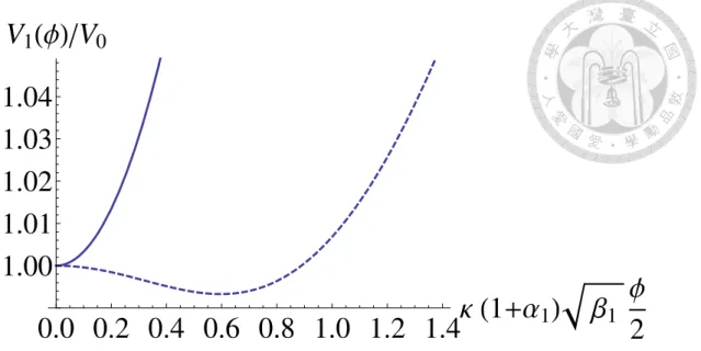
2.1 The scalar field potential for the NFDW era ( 1 = 1) for di↵erent values of ↵₁. The solid curve corresponds to ↵₁ = 1 (has unique minimum at = 0) and the dashed curve corresponds to ↵1 = 7 (has minimum at > 0). The situation is similar for the case of NFCS ( 1 = 2), which we omit here. . . 16 2.2 The scalar field potential for 1 = 1 (preinflationary NFDW). The

upward convex curve is V₁ (cf. Eq. (2.15)) and the downward cacave curve is V2 (cf. Eq. (2.16)). We can choose  0 for V¹ and 0 for V2 to describe the potential of the scalar field . In this model the scalar field rolls down too quickly in the slow-roll inflationary era and the radiation dominated phase is reached too early. . . 18 2.3 This plot shows the rescaled potentials given in Eqs. (2.23) and (2.25)

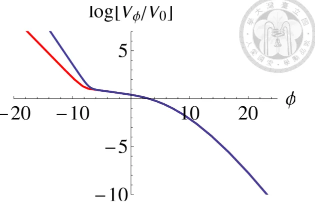
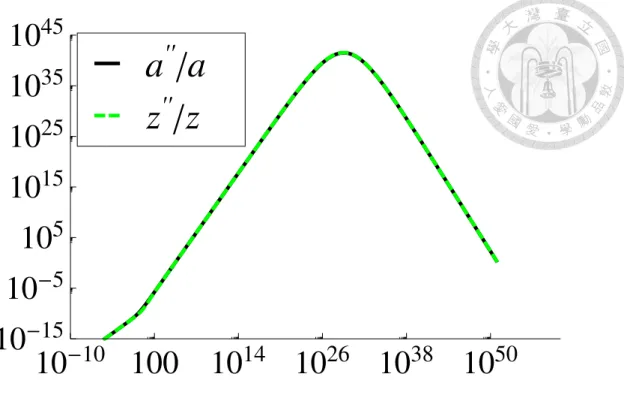
versus the scalar field , where V0 = A^1/(1+₂ ³⁾(A2/B2) ⁽¹⁺ ²^)/(q(1+ ³⁾⁾. The blue curve corresponds to the NFCS case, and the red curve corresponds to the NFDW case. The energy scale of inflation, V0, in our model is about 10¹⁵ GeV for both NFDW and NFCS. . . 21 2.4 The green dashed curve corresponds to z⁰⁰/z and the black curve cor-

responds to a⁰⁰/a. As can be seen that the approximation z⁰⁰/z ⇡ a⁰⁰/a holds during the NFDW dominated and the power-law inflationary eras. . . 23

(14)

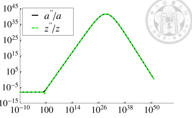
2.5 The green dashed curve corresponds to z⁰⁰/z and the black curve corresponds to a⁰⁰/a. As can be noticed that the approximation z⁰⁰/z ⇡ a⁰⁰/a holds during the NFCS dominated and the power-law inflationary eras. . . 24 2.6 This plot corresponds to the curvature perturbation spectrum for

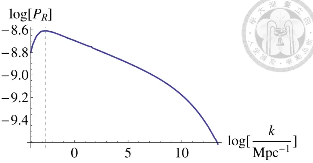
the inspired modified GCG model with ₁ = 1 (see Eq. (2.18a)), which describes a NFDW dominated era followed by a power-law inflationary period. We choose 3 = 1.05. The vertical dashed line corresponds to the pivot scale k = 0.002 Mpc ¹. . . 27 2.7 This plot corresponds to the curvature perturbation spectrum for the

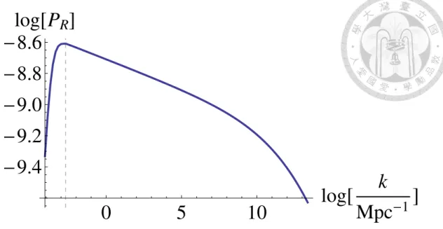
modified GCG model with 1 = 2 (see Eq. (2.18a)), which describes a NFCS dominated era followed by a power-law inflationary period.

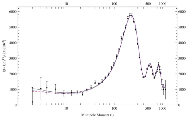
We choose 3 = 1.05. The vertical dashed line corresponds to the pivot scale k = 0.002 Mpc ¹. . . 28 2.8 The CMB temperature anisotropy spectrum. The dots with error

bars are the WMAP 7-year data. The solid line is the prediction of standard inflation with a power-law spectrum. The dashed and dotted lines are the spectra of the scenarios of NFCS and NFDW, respectively. . . 29

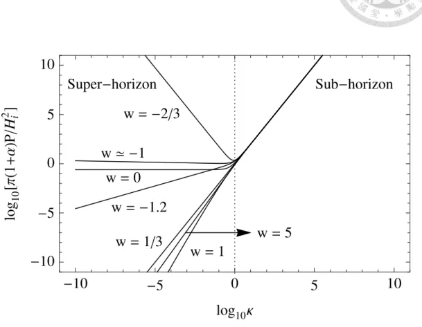
3.1 The power spectra (3.29) with sample parameters w = 1.2, 2/3, 0, 1/3, 1, 5, and at the slow-roll limit w ' 1. They are plotted with normalizations such that they have the same magnitude at the sub-horizon limit. For w ' 1 the power spectrum is given by (3.31), and the normalization is instead ⇡✏P/H_i². The complete relationship between the slope of the super-horizon spectrum and the equation- of-state parameter is described by the scaling relation (3.38), and is plotted in Figure 3.2. . . 40

(15)

3.2 The plot of 2µ + 3, the exponent of the power-law scaling relation (3.38) with respect to the equation-of-state parameter, w. . . 41

4.1 Time evolution of the power spectrum in era C in the case of single- stage evolution (only era C). The solid curves are the spectra of R from early time to late time (from light to dark). The vertical dashed lines denote the comoving horizon size at the corresponding instants (also from light to dark). . . 46 4.2 Time evolution of the power spectrum in era B in the case of two-

stage evolution (era B and C). The solid curves are the spectra of R from early time to late time (from light to dark). The vertical dashed lines denote the comoving horizon size at the corresponding instants (also from light to dark). . . 48 4.3 Time evolution of the power spectrum in era C in the case of two-

stage evolution (era B and C). The solid curves are the spectra of R from early time to late time (from light to dark). The vertical dashed lines denote the comoving horizon size at the corresponding instants (also from light to dark). . . 49 4.4 Illustration of the evolution of the physical wavelengths of the modes

and the Hubble radius with respect to the number of e-fold, N . The three parallel straight lines denote the modes with three di↵erent wavelengths, long to short from top to bottom (color online). The corresponding features they generate in the power spectrum, Figure 4.3, are labeled in the legends (top to bottom corresponding to long to short wavelengths). The black piecewise-connected lines denote the Hubble radius evolving from the kinetic era to the slow-roll era, and finally into the ⇤CDM era. The shaded region denotes the scales within which are causally connected. . . 51

(16)

4.5 Time evolution of the power spectrum in era B in the case of three- stage evolution (era A, B, and C). The solid curves are the spectra of R from early time to late time (from light to dark). The vertical dashed lines denote the comoving horizon size at the corresponding instants (also from light to dark). . . 53

4.6 Time evolution of the power spectrum in era C in the case of three- stage evolution (era A, B, and C). The solid curves are the spectra of R from early time to late time (from light to dark). The vertical dashed lines denote the comoving horizon size at the corresponding instants (also from light to dark). . . 54

4.7 Illustration of the evolution of the physical wavelengths of the modes and the Hubble radius with respect to the number of e-fold, N . The five parallel straight lines denote the modes with di↵erent wavelengths, long to short from top to bottom (color online). The corresponding features they generate in the power spectrum, Figure 4.6, are labeled in the legends (top to bottom corresponding to long to short wavelengths). The black piecewise-connected lines denote the Hubble radius evolving from the first slow-roll era to the kinetic era, then to the second slow-roll era, finally into the ⇤CDM era. The shaded region denotes the scales within which are causally connected. 56

4.8 Time evolution of the power spectrum in era S in the case of two- stage evolution (era S and C), with w = 1.2. The solid curves are the spectra of R from early time to late time (from light to dark).

The vertical dashed lines denote the comoving horizon size at the corresponding instants (also from light to dark). . . 58

(17)

4.9 Time evolution of the power spectrum in era C in the case of two- stage evolution (era S and C), with w = 1.2, NS = 6, and ✏ = 0.1.

The solid curves are the spectra of R from early time to late time (from light to dark). The vertical dashed lines denote the comoving horizon size at the corresponding instants (also from light to dark). . 59

5.1 The spectra of the curvature perturbations with i = 3.63MP, 3.65MP, and 3.67MP. The other parameters are held fixed as ⁰ = 10 ⁹,

i = 1.60MP, and m = 1.22⇥ 10 ⁶MP. . . 68

5.2 The CMB temperature-temperature correlation (TT) spectra with

i = 3.63MP, 3.65MP, and 3.67MP. The dots with error bars are the Planck 2013 data. The other parameters are held fixed as ⁰ = 10 ⁹,

i = 1.60MP, and m = 1.22⇥ 10 ⁶MP. . . 69

5.3 The CMB TT spectra with i = 1.50MP, 1.60MP, and 1.64MP. The dots with error bars are the Planck 2013 data. The other parameters are held fixed as ⁰ = 10 ⁹, _i = 3.65M_P, and m = 1.22⇥ 10 ⁶M_P. . 70

5.4 The CMB TT spectra with ⁰ = 10 ¹⁰, 10 ⁹, and 3⇥ 10 ⁹. The dots with error bars are the Planck 2013 data. The other parameters are held fixed as i = 3.65MP, i = 1.60MP, and m = 1.22⇥ 10 ⁶MP. . . 71

5.5 Time evolution of the power spectrum in era B in the case of three- stage evolution (era A, B, and C), in which w = 0 in era B. The solid curves are the spectra of R from early time to late time (from light to dark). The vertical dashed lines denote the comoving horizon size at the corresponding instants (also from light to dark). . . 74

(18)

5.6 Time evolution of the power spectrum in era C in the case of three- stage evolution (era A, B, and C), in which w = 0 in era B. The solid curves are the spectra of R from early time to late time (from light to dark). The vertical dashed lines denote the comoving horizon size at the corresponding instants (also from light to dark). . . 75

6.1 The power spectrum obtained by numerically solving the perturbations with ˜m = 0, H0 =p

8⇡/3. . . 89 6.2 The power spectrum obtained by numerically solving the perturba-

tions with ˜m = 1000p

0.1, H0 =p

8⇡/3. . . 89 6.3 The power spectrum obtained by numerically solving the perturba-

tions with ˜m =p

0.1⇥{0, 1, . . . , 10}, from top to bottom. All spectra are plotted with H0 =p

8⇡/3. . . 90 6.4 The time evolution of power spectrum in the case of ˜m = 0, H0 =

p8⇡/3. The darker curves correspond to the spectra at later times.

The lightest curve is the initial Lorentzian spectrum at time ti. For each n mode, the power is evaluated up to its horizon crossing time. . 91 6.5 The time evolution of power spectrum in the case of ˜m = 0.5H0,

H0 = p

8⇡/3. The darker curves correspond to the spectra at later times. The lightest curve is the initial Lorentzian spectrum at time ti. For each n mode, the power is evaluated up to its horizon crossing time. . . 92 6.6 The time evolution of power spectrum in the case of ˜m = H0, H0 =

p8⇡/3. The darker curves correspond to the spectra at later times.

The lightest curve is the initial Lorentzian spectrum at time ti. For each n mode, the power is evaluated up to its horizon crossing time. . 93

(19)

6.7 The time evolution of power spectrum in the case of ˜m = 2H0, H0 = p8⇡/3. The darker curves correspond to the spectra at later times.

The lightest curve is the initial Lorentzian spectrum at time ti. For each n mode, the power is evaluated up to its horizon crossing time. . 94

(20)

(21)

List of Tables

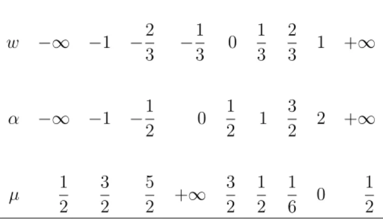
3.1 Corresponding values of ↵ and µ for some reference equation-of-state parameter w. The parameter ↵ = (1 + 3w)/2 is related to the scale factor by (3.13), and µ = |3(1 w)/2(1 + 3w)| describes the general solution of the perturbation through (3.16). Note that for the accelerating universe with w < 1/3, one has ↵ < 0, while for the decelerating universe with w > 1/3, one has ↵ > 0. . . 35

(22)

Chapter 1 Introduction

The ⇤CDM model of cosmology with an early inflationary era is very successful in explaining the cosmic microwave background (CMB) power spectrum. However, it has been observed in the COBE data that the quadrupole power is lower than the model prediction [1, 2]. This observation is further confirmed by WMAP, reporting the quadrupole power lower than the theoretical expectation by more than 1 but less than 2 [3]. Although this stand-alone low quadrupole mode may be explained by the cosmic variance, the Planck observation analyzed the low-` (` < 30) and high-` (` 30) spectra separately, and showed that the best-fit amplitude for the low-` spectrum is 10% lower than that for the high-` one at 2.5–3 significance [4, 5].¹

The CMB quadruple originates from the lowest modes of the primordial power spectrum with comoving wave number k of the order of 10 ³Mpc ¹. These lowest modes are the first modes that exit the horizon during inflation and the last ones that reenter in the radiation, matter, or dark energy dominated eras. Consequently, we expect that these modes are heavily a↵ected by the physics of the very early

1This low-`/high-` tension is present even when the particularly low quadrupole mode is ex- cluded from the analysis [4]. In [5] it is further pointed out that the low-` power deficit is mainly caused by the low multipoles between ` = 20 and 30.

(23)

universe, possibly the physics prior to the slow-roll inflationary era. Based on this reasoning, there have been attempts to explain the low-` power suppression of the CMB by introducing some preinflation era that breaks the slow-roll condition at about 60 e-folds before the end of inflation [6, 7, 8, 9, 10, 11, 12, 13, 14, 15]. The basic argument about how an era that deviates from the slow-roll dynamics could suppress the power is that the amplitude of the curvature perturbation,R ⇠ H / ˙, would decrease as | ˙| increases. This scenario is first realized in the single-field chaotic inflation with potential V = m^{2 2}/2, where m is the mass of the inflaton. If the inflaton starts with large speed ˙² m^{2 2}, the kinetic energy dominates the preinflation universe, and the power at the horizon scale is suppressed [6]. Other scenarios of violating the slow-roll evolution include the preinflation era filled with some radiation [7], the primordial black hole remnants [8], or the frustrated network of topological defects [9]. There are also preinflation models in which the universe is dominated by the spatial curvature as the emergent property from a number of moduli fields in the models of solid inflation [16, 10]. All of the models above report power suppression at the large scales.

On the other hand, the existence of the preinflation decelerating era in models that predict multi-stage inflation does not always result in power suppression [17, 18, 19, 11, 20, 12, 13, 14]. In the presence of two fields with mass hierarchy, there are two inflationary eras connected by a decelerating era. With the second inflationary era identified as the last 60 e-folds of the inflation, it is shown that the power is enhanced, rather than suppressed, at large scales that cross the horizon during the first inflationary era or the decelerating era [17]. Similar evolution also occurs in the early times of the hybrid inflation [21], in which the heavy field is played by the

“waterfall field” who acquires the mass through the coupling to the inflaton field.

In this case, it is however inferred that when the coupling term dominates at the early times, the inflaton field rolls faster due to the coupling, and eventually leads

(24)

to the power suppression [6]. Among other models of multi-stage inflation which commonly have a decelerating era before the last inflationary era, some predict power suppression at large scales [11, 12, 14], while some predict enhancement [17, 18, 19, 20, 13]. One therefore naturally wonders: What initial condition of inflation generated by the preinflation era would actually suppress the CMB power spectrum at large scales?

1.1 Topological Defects

As a toy model to study the preinflation era, we propose a new cosmological period just before the slow-roll inflationary era. This period corresponds to an era described by a network of topological defects, which we will assume to be frustrated domain walls or cosmic strings [22, 23, 24, 25, 26]. We expect that the production of topological defects at those scales follows the prediction of high energy physics.

In addition, given that the topological defects era precedes the slow-roll inflationary era, the topological networks will a↵ect mainly the lower modes of the power spectrum of the scalar and tensorial perturbations. Afterwards, they will soon be diluted during most of the inflationary era.

Topological defects such as domain walls or cosmic strings can naturally arise in the history of the universe. In a system that has spontaneous symmetry breaking, the symmetry that is broken at low temperature is restored at high temperature.

The standard model of the elementary particles has such scenarios including the electro-weak and GUT (grand unified theory) scale symmetry breaking. In the early universe, when the temperature is higher than the symmetry breaking scale, the field is in a global minimum (with quantum fluctuation around the minimum).

As the universe expands, the temperature will eventually drop below the critical temperature associated with the symmetry. In the low temperature, the potential of the field has multiple degenerate vacua, and the field will fall down to one of the

(25)

vacua randomly. Across the space in the universe, there are therefore many spatial regions in which the field drops to di↵erent vacua. Two regions in di↵erent vacua are separated by a domain wall, usually in the case of the discrete symmetry. Cosmic strings can arise from the breaking of a local U (1) symmetry in the Abelian Higgs model, which allows the solution of vortex lines [27].

Topological defects are interesting subjects in cosmology for several reasons.

An early one is that it could possibly seed the large-scale structure we observe today. Planar domain walls, for example, repel the baryonic matter and induce inhomogeneities [28]. However, if the domain walls are produced too early in the history of the universe, their energy density may dominate over the other radiation and baryonic matter sources and significantly alter the observed expansion history.

On the other hand, if the domain walls are created at lower energy scales, while their energy density will be subdominant, the kinetic energy of them may still spoil the isotropy of the CMB we observe today.

The network of frustrated domain walls and cosmic strings are considered to be viable components of the universe because they will not destroy the isotropy of CMB [29], nor cluster at the small scale [22]. This is because the network structure makes the domain walls behave like some kind of solid, whose elastic resistance is only shear deformations. It is hard to have large kinetic movement in orders higher than the bulk velocity. Moreover, due to their topological nature, the pressure of such networks of topological defects is negative and of the same order of their energy density, so their speed of sound is close to the speed of light. As a consequence, their Jeans length is comparable to the size of the horizon, and they does not collapse at small scales. One example of the network of domain walls joined by cosmic strings is given by the complex U (1) scalar field, such as axions [28]. In this type of simple models the string and anti-directed string will soon annihilate each other within the Hubble radius, therefore unable to form the stable network structure. To maintain

(26)

a network structure, one can instead consider, for example, the O(N ) field [28], which has di↵erent types of cosmic strings. In this scenario, the probability of pair- annihilations of the cosmic strings are suppressed because the same type of strings collide less frequently.

1.2 Relation between initial state and power spec- trum

One of our most important findings is that, in general, the long-wavelength spectrum at the end of inflation reflects the super-horizon spectrum of the initial state [30].

To establish such relationship between the initial state and the power spectrum, we first find the spectrum of the adiabatic vacuum in the universe with a constant equation of state driven by a scalar field. The conditions of having the blue-tilted, red-tilted, or scale-invariant spectra at the super-horizon scales are found. The spectra obtained are based on the assumption that the mode solutions approach the Minkowski limit at small scales. We point out that in the decelerating universe the super-horizon modes would enter the horizon and become sub-horizon, which means that these super-horizon modes are initially causally disconnected. Such assumption in an initially decelerating universe therefore relies on the final state of the mode evolution to govern its initial state, which reverses the cause and e↵ect. Later it was shown that the large-scale power suppression in models with preinflation decelerating era is actually a consequence of this unnatural yet widely adopted assumption.²

In the next step, we demonstrate that for the universe experiencing several eras

2Such a choice of the initial state for inflation, often referred to as the Bunch-Davies vacuum, even if there exists a non-slow-roll preinflation phase, has been commonly assumed in the literature (see, for example, [6, 18, 7, 13, 9, 15, 10]). There also exist numerous proposals of a non-Bunch- Davies vacuum as the basis of the initial condition for a universe that does not begin with a slow-roll phase (see, for example, [31, 32, 33, 34]).

(27)

with di↵erent equations of state, the large-scale spectrum is determined by the earliest era in which the universe begins. Starting with a single slow-roll era with the scale-invariant super-horizon spectrum, we find how the spectrum changes as one incrementally stacks a kinetic era, and yet another slow-roll era, into the early times.³ If the universe begins with the initial adiabatic vacuum in the kinetic era, the spectrum is suppressed at large scales, and we find that the suppression is a direct consequence of the blue-tilted super-horizon spectrum in the initial kinetic era. With another slow-roll era preceding the kinetic era, the large-scale spectrum is enhanced because the super-horizon spectrum in the initial slow-roll era is scale-invariant with the amplitude higher than that generated in the second slow-roll era. In this case, the intermediate kinetic era only serves to connect the two scale-invariant spectra of the two slow-roll eras. One sees that the power suppression stems from the initial blue-tilted super-horizon spectrum, and once the initial spectrum is di↵erent, the large-scale power may not be suppressed even if there is a preinflation kinetic phase.

We also investigate the scenario that the universe starts with a superinflation era before the slow-roll inflation. The superinflation era can be induced in theories of quantum gravity [36, 37, 15, 38], or by a scalar field that violates the dominant energy condition [39, 40]. Models in the latter case generally su↵er from quantum instabilities and should only be regarded as e↵ective theories (for related discussions, see, for example, [41, 42]). The interest here lies in the fact that, opposite to the case of a single preinflation kinetic era, it is causal to assume the initial adiabatic vacuum in the preinflation superinflation era. We found that in this case the large- scale power is also suppressed due to the blue-tilted super-horizon initial spectrum in the superinflation era. Power suppression due to an early superinflation era has also been inferred in the models of loop quantum gravity [36] or bouncing cosmology [15], while in this work a more systematic treatment to the evolution of perturbations is

3The e↵ect due to piecewise changes of the model parameter was studied in [35], where the time-dependent e↵ective inflaton mass was considered.

(28)

given.

After understanding the character of the spectrum in the multi-stage inflation using the ad hoc single-field analysis, we calculate the spectrum of the curvature perturbations in a two-field model with the given potential. We consider the chaotic potential with a coupling term to the second scalar field, which is similar to the e↵ective potential in the early stage of the hybrid inflation. By numerically solving the equations of motion and using the CAMB code [43, 44], we show that the large- scale spectra of curvature perturbations and CMB are indeed enhanced due to the initial inflationary era.⁴

1.3 Initial Condition from Quantum Cosmology

As we showed earlier that the power suppression can occur if one of the two following possibilities happens in the early stage of the inflation: First, the phantom equation of state (and the superinflationary expansion due to the phantomness) can induce the power suppression. Second, a positive-pressure era (with the equation-of-state parameter w > 0), such as the kinetic-energy-dominated era, at the early stage of inflation can cause the power suppression. Both scenarios are logically possible, but both ideas have their own problems. For the phantom inflation scenario, it is very difficult to construct a viable theory for the phantom matter. For the positive- pressure era, the power suppression highly depends on the choice of the vacuum state. In the de Sitter space, we have a canonical choice of the vacuum—the Bunch- Davies vacuum [45], but in the positive-pressure era, there is no such a canonical

4As regards the treatment of the two-stage inflation, our approach is closest to that of [18, 19], in which a more complicated string-motivated two-field model is considered. In [17] the two fields have no direct coupling, and certain approximations are used to obtain the analytical solutions in various regimes of the model parameters. In [11, 12, 14, 20], the single-field models are used. In [13] the system is also modeled by a single fluid.

(29)

vacuum. Moreover, if we consider an eternally inflating background (and the con- sequent Bunch-Davies vacuum), then even though the universe evolves toward a positive-pressure era, the power suppression will not be realized [30].

The existing difficulties of having a consistent explanation for the power suppression may imply that its origin does not lie in the semi-classical physics, but in the quantum theory of gravity. Can we explain the power suppression by quantum gravitational e↵ects? Indeed, there has been several models explaining the power suppression from quantum gravity. For example, according to the loop quantum cosmology, quantum gravitational e↵ects can induce an e↵ective phantom matter in the deep trans-Planckian regime. The phantomness thereof can explain the CMB power suppression as well as supporting the scenario of the big bounce universe [46].

In order to investigate the wave function of our universe and the power suppression problem, we will rely on the Hartle-Hawking wave function, or the so-called no-boundary wave function [47]. This wave function is one of the proposals to the boundary condition of the Wheeler-DeWitt equation [48]. It is a path integral over the Euclidean compact manifolds, and can be approximated by the method of steep- est descent. Under such approximation, we can then describe the wave function as a sum of the Euclidean instantons, where each instanton should eventually be Wick- rotated into the Lorentzian signatures [49, 50] and approach real-valued functions [51, 52, 53, 54, 55]. By integrating the Lagrangian, one can estimate the probability for the history described by each instanton.

Following the work of Halliwell and Hawking [56], one can introduce perturbations to the background instanton solution. These perturbations also carry their own canonical degrees of freedom. Although in general it is very difficult to track their coupled evolution, one can consistently consider various modes separately as long as the perturbations stay in the linear regime. The probability distribution of the magnitude of each perturbation mode can then be calculated, and the expec-

(30)

tation values of these modes, or equivalently, the power spectrum, can therefore be determined.

Using the method of Laflamme [57], we can define the wave function for the Euclidean vacuum. The Euclidean vacuum gives the scale-invariant power spectrum at short-wavelength scales, hence consistent with the choice of the Bunch-Davies vacuum [45] at small scales. On the other hand, at the long-wavelength scales, the power spectrum is enhanced due to the curvature of the manifold. All these results have been known in the literature and consistent with the independent calculations from quantum field theoretical techniques [58, 59]. However, to our best knowledge, it was not emphasized that the power spectrum can be suppressed by introducing the potential term. In chapter 6, we include analytical and numerical details for the power suppression due to the potential term of the inflaton field [60].

We adopt the Planck units (c = ~ = G = 1) and the signature ( , +, +, +) throughout the thesis.

(31)

(32)

Chapter 2 Preinflationary Network of

Frustrated Topological Defects

One natural candidate that may cause the power suppression at the lowest modes of the CMB spectrum is the primordial topological defect produced during some phase transition in the preinflationary era. If the universe is populated with the topological defects before the slow-roll inflation, the expansion rate of the preinflationary universe is generally di↵erent from that of the de Sitter universe. Therefore, the curvature perturbations evolves di↵erently in the preinflationary era from the way they do in the inflationary era. If inflation sustains for just about 60 e-folds, we can then see the imprint of the transition from the preinflationary to the inflationary era on the perturbation spectrum.

In this chapter we consider two of the most common types of topological defects—

domain walls and cosmic strings—arising from the phase transitions at the cosmic scale. To model the transition from the preinflationary to the inflationary era, we introduce the generalized Chaplygin gas (GCG) [61, 62, 63, 64, 65]. The idea of describing the early universe by the Chaplygin gas was first suggested in Refs. [66, 67]

(see also [68, 69]) and later extended in Refs. [70, 71, 72, 73, 74, 75]. The energy density of a network of frustrated topological defects (NFTD) can be described in

(33)

a compact way, for example, as

⇢ =

✓ B1

a ¹^(1+↵¹⁾ + A1

◆1/(1+↵1)

, (2.1)

where a is the scale factor, B1 and A1 are constants related to the energy scale of the NFTD and the de Sitter-like inflationary era, respectively, ↵1 and 1 are constants such that 1 = 1, 2 for the network of frustrated domain walls (NFDW) and the network of frustrated cosmic strings (NFCS), respectively. We assume that 1 + ↵1

is positive such that the inflationary era is preceded by a topological dominance phase. Let us be reminded in this regard that the energy density of NFDW and NFCS scales as 1/a and 1/a², respectively [27]. It is worthy to stress that the NFTD epoch preceding the slow-roll inflationary can in principle produce inflation as well;

indeed this is the case for NFDW, but this inflation is much slower, i.e. much lazier than the slow-roll inflation. Moreover, for a NFCS dominated period the universe is increasing its size at a constant speed; i.e. with no acceleration or deceleration.

From now on whenever we refer to a preinflationary era, we will be referring to a pre-slow-roll inflationary era.

We consider a spatially flat Friedmann-Lemaˆıtre-Robertson-Walker (FLRW) universe filled with the matter content described by Eq. (2.1). The energy conservation gives

˙⇢ + 3H(⇢ + p) = 0, (2.2)

where a dot corresponds to a derivative with respect to the cosmic time and H stands for the Hubble rate. By inserting Eq. (2.1) into Eq. (2.2), one obtains the pressure of the matter content

p =

✓

1

3 1

◆

⇢ ¹

3 A₁

⇢^↵¹. (2.3)

Note that in terms of the equation of state,

p = w⇢, (2.4)

(34)

where w is the equation-of-state parameter, the universe is in the state of w = 2/3 and w = 1/3 for = 1 (NFDW dominated) and = 2 (NFCS dominated), respectively.

In the Planck unit, the Friedmann equation reads

H² = ²

3 ⇢, (2.5)

where ² ⌘ 8⇡G = 8⇡. The conformal time ⌧ can be expressed as

⌧ = p3

 b

cA₁^(b+c)

✓B1

A1

◆b

y^c ₂F₁(c, 1 b, c + 1, y), (2.6)

where y = ⇥

1 + (B1/A1) a ¹^(1+↵¹⁾⇤ 1

, b = 1 /[ 1(1 + ↵1)] , c = ( 2 + 1)/[2(1 +

↵1) 1], and 2F1 is a hypergeometric function [76]. Eq. (2.6) describes that the universe began in NFTD dominated era in the past infinity, and turned into a de Sitter-like space, in which a/ 1/⌧, at later time.

2.1 Model Building and Parameters Fixing

We divide the expansion of the universe into three successive periods: the preinflationary NFTD dominated era, the slow-roll inflating phase, and the standard ⇤CDM epoch. The energy density of each of these periods can be modeled as

⇢ = 8>

>>

<

>>

>:

 B₁

a ¹^(1+↵¹⁾ + A1

1/(1+↵1)

, (2.7a)



A2+ B2

a^4(1+↵²⁾

1/(1+↵2)

, (2.7b)

⇢_r0⇣a0

a

⌘4

+ ⇢_m0⇣a0

a

⌘3

+ ⇢_⇤. (2.7c)

Expression (2.7a) describes the energy density of the NFTD era, which was in- troduced in Eq. (2.1), followed by the de Sitter-like inflating phase. The model described by Eq. (2.7b) was previously studied within an inflationary framework in Ref. [70, 71] (see also Ref. [65]) and, under suitable constraints on A2, B2, and

↵2, can depict the transition from the de Sitter-like era to the radiation dominated

(35)

era. The energy density (2.7c) is the standard ⇤CDM model, in which ⇢r0, ⇢m0, and ⇢⇤ are the energy densities of the radiation, matter, and dark energy today, respectively. As we will show later, the parameters of the model can be constrained using observational data corresponding to the present energy density of radiation, the scalar power spectrum, and the spectral index at a given pivot scale. In addition, by requiring that the energy density is continuous at each transition, we have the conditions

A1 = A^(1+↵₂ ¹^)/(1+↵²⁾, (2.8)

B₂ = ⇢_r0a⁴₀ ^1+↵². (2.9)

In order to obtain the scalar power spectrum, it is useful to model the matter content in the first two periods of Eq. (2.7); i.e. those described by Eqs. (2.7a) and (2.7b), through a scalar field, with the condition that the energy density and pressure of the scalar field are the same as that given by Eqs. (2.7a) and (2.7b). The energy density and pressure of the scalar field are

⇢ =

02

2 a² + V ( ), p =

02

2 a² V ( ), (2.10)

where the primes denote the derivatives with respect to the conformal time. The scalar field and its potential in the first period is given by

(a) = 1

 (1 + ↵1)p

1

⇥ ln 0

@ 1 +q

1 + (_B^a

1/A1) ¹^(1+↵¹⁾ 1 +q

1 + (_B^a

1/A1) ¹^(1+↵¹⁾ 1

A , (2.11)

V1(a) =V0

6 8<

:(6 1)

"

1 +

✓B1/A1

a ¹

◆(1+↵1)#1/(1+↵1)

+ ₁

"

1 +

✓B1/A1

a ¹

◆(1+↵1)# ↵1/(1+↵1)9

=

;, (2.12)

where V0 = A^1/(1+↵₁ ¹⁾. Similarly, the scalar field and its potential in the second period can be obtained by replacing ↵1 with ↵2 and setting 2 = 4 in Eq. (2.11) and

(36)

Eq. (2.12), giving

(a) = 1

2 (1 + ↵2)

⇥ ln 0

@ 1 +q

1 + (_B^a

2/A2)^4(1+↵²⁾ 1 +q

1 + (_B₂^a_/A₂)^4(1+↵²⁾ 1

A , (2.13)

V2(a) =V0

3 ("

1 +

✓B2/A2

a⁴

◆(1+↵2)#

1/(1+↵2)

+2

"

1 +

✓B2/A2

a⁴

◆(1+↵2)# ↵2/(1+↵2)9

=

;. (2.14)

We can obtain the potential of the scalar field for the two periods as functions of the scalar field by substituting the inverse function of Eq. (2.11) into Eq. (2.12) and similarly that of Eq. (2.13) into Eq. (2.14), respectively, which leads to

V1( ) = V0

6 (

(6 1) cosh



 (1 + ↵1)p

12

2 1+↵1

+ 1cosh



 (1 + ↵1)p

12

1+↵12↵1)

, (2.15)

V2( ) = V0

3 n

cosh [ (1 + ↵2) ]^1+↵2² +2 cosh [ (1 + ↵2) ]^1+↵2^2↵2o

. (2.16)

Eq. (2.16) coincides with the potential in Ref. [70, 71], as it should be. The form of Eq.(2.15) and Eq.(2.16) has been chosen such that the two periods are connected at

= 0 with the potential and its first derivative with respect to being analytically continuous at the connecting point. The result is shown in Figure 2.2.

Next we tackle the issue of analyzing the potentials (2.15) and (2.16). First of all, we consider that the scalar field potential (2.15) has a unique minimum at = 0 to maximize the amount of inflation during the first period. Notice that unless this condition is imposed, the scalar field might roll down the potential till it reaches the minimum of V1( ) and then would have to climb up to reach the local maximum

(37)

0.0 0.2 0.4 0.6 0.8 1.0 1.2 1.4 Κ !1"Α

1

" Β

1

Φ 2 1.00

1.01 1.02 1.03 1.04

V

₁

!Φ"#V

⁰

Figure 2.1 The scalar field potential for the NFDW era ( 1 = 1) for di↵erent values of ↵1. The solid curve corresponds to ↵1 = 1 (has unique minimum at = 0) and the dashed curve corresponds to ↵₁ = 7 (has minimum at > 0). The situation is similar for the case of NFCS ( 1 = 2), which we omit here.

located at = 0, as shown in Figure 2.1. Imposing that the potential (2.15) has a unique minimum reached at = 0 implies a condition on the parameters ↵1 and 1

that

↵1 < 6 1 1

. (2.17)

Therefore, bearing in mind that (i) 1 = 1, 2 for NFDW and NFCS, respectively, and (ii) 0 < 1 + ↵1 so that the phase of FNTD precedes the inflationary phase, we conclude that 1 < ↵₁ < 5 for NFDW and 1 < ↵₁ < 2 for NFCS. We show the shape of the potential V1( ) for di↵erent cases when the condition (2.17) is fulfilled and violated in Figure 2.1.

In addition, we can constrain our model, potentials (2.15) and (2.16), using the methodology in Ref. [70, 71]. More precisely, we can use the WMAP7 observation of the power spectrum of the comoving curvature perturbation, Ps = 2.45⇥ 10 ⁹, and the spectral index, ns = 0.963, at the pivot scale k0 = 0.002 Mpc ¹ to fix the parameters in our model [77]. We can as well impose a bound on the number of

(38)

e-folds, Nc, since a given mode exits the horizon until the end of inflation as done in Ref. [70, 71]. This gives the best-fit values for ↵2, V0, and, therefore, A2. Notice that once V0is fixed, the parameter A1is fixed for a given ↵1 as well, since V0 = A^1/(1+↵₁ ¹⁾. The parameter B1 in Eq. (2.7a) fixes the energy density of the NFTD, which strongly a↵ects the lowest modes that exited the horizon around the onset of inflation, and causes a significant drop on the lowest modes of the primordial spectrum of the curvature perturbation. Although we expect that the NFTD would a↵ect the lowest modes, we must make sure that the curvature power spectrum Ps and the spectral index ns at the pivot scale k0 are consistent with the observations. There- fore, we choose the value of B1 such that Ps and ns match the observed values at k0, and that the amplitude of P_s drops at the scales whose comoving wave numbers are smaller than k0. Roughly speaking, the parameter B1 controls the horizontal shift of the curvature power spectrum.

However, following this procedure, it turns out that we can not find a set of values for the parameter B1 that satisfies the constraint on the spectral index. In fact, in this model B1 turns out to be always smaller than 0.9. This drawback originates from the second period described by Eq. (2.7b), which corresponds to the transition from the slow-roll inflationary era to the radiation dominated period.

More precisely, the model described by Eq. (2.7) does not give enough e-folds during the slow-roll inflationary era. We show, as an example, in Figure 2.2 how the scalar field rolls too quickly and the radiation dominated phase is reached too early in the case corresponding to a NFDW.

We therefore suggest an alternative model described by

⇢ = 8>

>>

<

>>

>: B1

a ¹ +

✓ A2

a¹⁺ ²

◆1/(1+ 3)

, (2.18a)

 A2

a¹⁺ ² + B2

a⁴⁽¹⁺ ³⁾

1/(1+ 3)

, (2.18b)

⇢r0

⇣a0

a

⌘4+ ⇢m0

⇣a0

a

⌘3+ ⇢⇤, (2.18c)

where 1 = 1, 2 discriminates the NFDW and the NFCS as in the former model,

(39)

!4 !2 0 2 4 Φ 0.5

1.0 1.5

V _Φ !V 0

V

₁

!V

0

V

₂

!V

0

Figure 2.2 The scalar field potential for 1 = 1 (preinflationary NFDW). The upward convex curve is V1 (cf. Eq. (2.15)) and the downward cacave curve is V2

(cf. Eq. (2.16)). We can choose  0 for V¹ and 0 for V2 to describe the potential of the scalar field . In this model the scalar field rolls down too quickly in the slow-roll inflationary era and the radiation dominated phase is reached too early.

and ₂, ₃, B₁, A₂, B₂ are constants we will explain below. The major di↵erence of this model from out previous one is that here we model the slow-roll inflation by a power-law expansion. We choose this model because it generates an almost flat curvature spectrum for modes larger than the pivot scale k0 = 0.002 Mpc ¹ and gives enough e-folds during the power-law inflationary period. In addition, the model introduces in a natural way that a NFTD precedes the power-law inflation as (1 + ₂)/(1 + ₃) < ₁ (please see also the conditions (2.19), (2.20) and (2.21)).

The first period in Eq. (2.18a) describes the matter content of the universe during a period that transits from a NFTD dominated phase to a power-law inflationary

(40)

era. The parameters B1 and A2 are associated with the energy scale of the NFTD and that of the power-law inflation, respectively. The second period with the energy density (2.18b) was previously studied within another inflationary framework in Ref. [72, 73]. It connects smoothly a power-law inflating phase with a radiation dominated universe, and the constraints on the parameters ₂ and ₃ are,¹

1 + 2 < 0, (2.19)

1 + 3 < 0, (2.20)

2(1 + ₃) < 1 + ₂. (2.21)

These constraints imply that (i) there is a power-law inflating phase, (ii) the inflationary era precedes the radiation dominated period, and (iii) the null energy condition is always fulfilled so that there is no superinflationary phase. Finally, the energy density described by (2.18c) corresponds to the ⇤CDM model as that described by Eq. (2.7c).

Although there seems to be many free parameters, they can be fixed down to only one by the following procedure: (i) Fix B2 by the current amount of radiation for a given 3. (ii) Constrain the power-law expansion quantified by A⁽¹⁺₂ ³^)/(1+ ²⁾ by the WMAP7 data of the curvature power spectrum Ps and the spectral index n_s. Since there are three parameters (A₂, ₂ and ₃) to be constrained by only two conditions (P_s and n_s), we are left with the only one free parameter, which we choose to be 3. (iii) Fix B1 such that Ps and ns remain the correct values at the pivot scale k0, and Ps drops only at comoving wave numbers smaller than k0.

Again, it is suitable to introduce a scalar field that mimics the matter content described in Eqs. (2.18a) and (2.18b); i.e. we describe the dynamics of the model through a scalar field with a potential whose energy density and pressure can be obtained from Eq. (2.10). During the NFTD period (cf. Eq. (2.18a)), the mapping

1The notation is di↵erent from the one used in the work [72, 73]. The parameters and ↵ in Ref. [72, 73] are denoted as 2 and 3here, respectively.

(41)

between the scalar field and the perfect fluid of our model leads to

(a) = p

v coth ¹ r

1

p v

1tanh ¹ r

⇣ + (1 ⇣) v

1

, (2.22)

V₁(a) = 1 6

"✓

5 + ³ ² 1 + 3

◆ ✓ A2

a¹⁺ ²

◆ ¹

1+ 3

+ (6 1)B1

a ¹ , (2.23)

where ⇣ = [1 + (A^1/(1+₂ ³⁾/B1)a ¹ ^v] ¹, v = (1 + 2)/(1 + 3), and V1( ) stands for the scalar field potential during this period. Similarly, we map the perfect fluid with the energy density (cf. Eq. (2.18b)) to the scalar field with a new potential V₂( ) [72, 73]

(a) = 1 q

"

4 tanh ¹ s

1 + q

4(1 + ₃) 1 1 + ⇠ 2 p⇣ coth ¹

s4

⇣

✓

1 + q

4(1 + 3) 1 1 + ⇠

◆#

,

(2.24) V2(a) = A^1/(1+₂ ³⁾

✓A2

B2

◆ ⇣/q

(1 + ⇠)^1/(1+ ³⁾

⇠ ^⇣/q

✓1 3

q 6(1 + 3)

1 1 + ⇠

◆ ,

(2.25)

where ⇠ = (B2/A2)a^qand q = 1 + 2 4(1 + 3). The potential (2.25) was previously obtained in Ref. [72, 73]. Such a potential, with an appropriate initial condition, drives a power-law inflation and mimics a radiation dominated universe afterwards.

Unlike the previous model described by Eq. (2.11)-(2.12) and Eq. (2.13)-(2.14), here it is not feasible to find analytically the inverse functions of Eq. (2.22) and Eq. (2.24), so we cannot obtain the analytical forms of the potential as functions of . We thus connect the scalar field potential numerically. V1(a) and V2(a) are connected at the intersection of the first two periods (Eq. (2.18a) and Eq. (2.18b)),

(42)

Figure 2.3 This plot shows the rescaled potentials given in Eqs. (2.23) and (2.25) versus the scalar field , where V₀ = A^1/(1+₂ ³⁾(A₂/B₂) ⁽¹⁺ ²^)/(q(1+ ³⁾⁾. The blue curve corresponds to the NFCS case, and the red curve corresponds to the NFDW case. The energy scale of inflation, V0, in our model is about 10¹⁵ GeV for both NFDW and NFCS.

where the second term of Eq. (2.18a) dominates over its first term, and the first term of Eq. (2.18b) dominates over its second term so that the potential and its first derivatives with respect to are approximately continuous at the intersection of the first two periods. It is worthy to notice that an integration constant appears when we integrate Eq. (2.10) after mapping it to the energy density and pressure of a given perfect fluid. Therefore, we can always choose the constant properly such that the scalar field is continuous at the connecting point. As a result, we can use the scale factor a as a parametric parameter to plot V1( ) and V2( ), which are shown in Figure 2.3 as an example. The scalar field starts with a negative value and rolls down the potential as the universe inflates until it reaches the radiation dominated era.

(43)

2.2 Scalar Perturbations

The accelerated expansion of the universe during the primordial inflationary era con- verts the initial quantum fluctuations in the universe into macroscopic cosmological perturbations, which leads to the inhomogeneity we observe nowadays in the CMB [78, 79]. Following the standard approach, we will use gauge invariant quantities that involve the metric perturbations and the scalar field fluctuations [80]. For con- venience, we will choose the comoving curvature perturbation, R, which in addition is conserved on large scales [81, 82].

We expect that a NFTD in the very early universe and just before the inflationary era could give the appropriate corrections to the quadrupole modes of the CMB data as observed nowadays [77]. We will next quantify the quantum cosmological perturbations during that period and obtain the power spectrum of the scalar perturbations.

The scalar perturbations can be described by introducing the variable (see, for example, Ref. [83])

u = zR, (2.26)

where z ⌘ ^{a ˙}_H. The variable u can be decomposed into Fourier modes, uk, which fulfill the field equation [83]

d²uk

d⌧² +

✓ k² 1

z d²z d⌧²

◆

u_k= 0. (2.27)

The modes uk can be mapped to the spectrum of the comoving curvature perturbations which reads [83]

2⇡²

k³ P_R(k) = |u^k|²

z² . (2.28)

Given that we are dealing with adiabatic perturbations, the comoving curvature perturbations remain constant on large scales and consequently we can equate the power spectrum at the horizon exit with the power spectrum of the primordial scalar perturbations at the horizon reentry as observed on the CMB. Therefore, for a given

(44)

10 ^!10 100 10 ¹⁴ 10 ²⁶ 10 ³⁸ 10 ⁵⁰ 10 ^!15

10 ^!5 10 ⁵ 10 ¹⁵ 10 ²⁵ 10 ³⁵ 10 ⁴⁵

z ^'' !z a ^'' !a

Figure 2.4 The green dashed curve corresponds to z⁰⁰/z and the black curve corresponds to a⁰⁰/a. As can be seen that the approximation z⁰⁰/z ⇡ a⁰⁰/a holds during the NFDW dominated and the power-law inflationary eras.

mode k, the spectrum is evaluated at the horizon exit; i.e. when k = acrossH, where across stands for the value of the scale factor when the mode exists the horizon.

We next obtain the evolution of the mode function uk(⌧ ) for each comoving wave number k in order to obtain the curvature perturbation spectrum. We will tackle this issue numerically rather than using the standard results for slow-roll inflation [78, 84, 83], because those conditions are not fulfilled at very early time when the NFTD is dominant. It is easier to solve Eq. (2.27) numerically by splitting it into two first order di↵erential equations,

8>

><

>>

:

X⁰ = Y

Y⁰ = k² ^z_z⁰⁰ X,

(2.29)

where we have set X = uk.

In addition, we need to impose a set of boundary conditions at the time when the wavelength of a given mode k is much smaller than the Hubble radius; that is,