基因及螞蟻規則探勘模式---以事故分析及事故鑑定為例

(1)

行政院國家科學委員會補助專題研究計畫

□ 成果報告

5期中進度報告

附件一

基因及螞蟻規則探勘模式-以事故分析及事故鑑定為例 (I/III)

Developing Genetic and Ant-based Rule Mining Models- Case

Studies on Accident Analysis and Appraisal (I/III)

計畫類別：5 個別型計畫 □ 整合型計畫

計畫編號：NSC 97-2628-E-009-035-MY3

執行期間：97 年 8 月 1 日至 100 年 7 月 31 日

計畫主持人：

邱裕鈞交通大學交通運輸研究所副教授

計畫參與人員：

陳彥蘅、傅強交通大學交研所博士班研究生

林柏辰、謝志偉

交通大學交研所碩士班研究生

成果報告類型(依經費核定清單規定繳交)：5精簡報告 □完整報告

本成果報告包括以下應繳交之附件：

□赴國外出差或研習心得報告一份

□赴大陸地區出差或研習心得報告一份

□出席國際學術會議心得報告及發表之論文各一份

□國際合作研究計畫國外研究報告書一份

處理方式：除產學合作研究計畫、提升產業技術及人才培育研究計畫、列

管計畫及下列情形者外，得立即公開查詢

□涉及專利或其他智慧財產權，□一年□二年後可公開查詢

執行單位：國立交通大學

中華民國 98 年 5 月 25 日

(2)

一、摘要

1.1 中文摘要

本計畫第一年期之研究內容旨在利用規則探勘模式（genetic rule mining, GRM），建立一套事故鑑定專家系統，除可供事故責任鑑定之精確預測外，並提供學習所得規則，供進一步詮譯、後最佳化及訓練之用。本研究共提出三種 GRM 模式，並利用民國 89～91 年之事故鑑定案例，共計 537 件，1,074 位當事人作為研究對象，透過卡方檢定共評選出 22 個關鍵鑑定變數，以作為潛在之狀態變數，控制變數則設定為鑑定責任（分別全因、主因、次因、同為及無因等五個等級）。所有變數均設定為類別變數（categorical variables），俾利變數數值之選擇。至於 GAs 染色體之編碼，則以每一條染色體代表一條邏輯規則，每一族群代表所組成之邏輯規則組成。各染色體之適合度值（fitness value）則以三個目標表之，分別為：包含事故件數最多、與其他染色體重覆最少、與其他染色體矛盾度最低。並與類神經網路及判別分析方法進行績效評比。結果顯示，本模式之判中率明顯高於類神經網路及判別分析模式，且所選擇之邏輯規則也可據以了解鑑定委員之推理邏輯。另外，本年期也進一步將所建構之 GRM 模式應用於高速公路事故嚴重度之分析。為避免三級嚴重度之事故件數分佈不均所導致之過度挖掘問題，本研究乃以隨機方式選擇相同數量之事故件數進行模式訓練與驗證，並將預測結果與決策樹比較，以驗證本模式之績效。結果顯示，本模式共計選擇了 19 條規則，其訓練準確度達 78.50%，而驗證準確度則達 74.16% 均遠高於決策樹之預測結果。而障礙物及鋪面狀況是兩個最重要的影響事故嚴重度之成因。關鍵字：事故鑑定、規則探勘、遺傳演算法、事故嚴重度 1.2 Abstract

The first research year of this project aims to propose an accident appraisal expert system that can not only accurately predict the liability degrees of involved parties but also demonstrate comprehensive appraisal rules for further investigation, post-adjustment, and training of junior accident appraisal committee members. Three genetic rule mining (GRM) models, based on two schemes of the Michigan approach (GRM1 and GRM2) and on the Pittsburgh approach (GRM3) are respectively proposed by discovering knowledge from historical appraisal cases. A total of 537 Taiwanese two-car crash accident cases (1,074 parties) are randomly and equally divided into three subsets to train and validate the proposed models. The GRM1 model performs the best in both training and validation with correctness rates of 78.85% and 70.21%, respectively. We further compare the proposed GRM1 model with artificial neural network models (ANN) and discrimination analysis (DA) model proposed by Chiou (2006). The GRM1 model can achieve the same accuracy as the ANN models and provide more information than the ANN models by delivering a comprehensive combination of rules. It can be used to enhance the quality and efficiency of accident appraisal.

In addition, the proposed GRM models have also been applied to freeway accident analysis to discover the key rules that determine the most contributing factors to crash severity. To avoid over-mining caused by unevenly distributed data across different types of accidents, identical numbers of A1-type, A2-type, and A3-type crash cases drawn from 2003-2007 Taiwan freeway accident investigation reports are used for the analysis. A total of 19 rules have been mined which can achieve overall correct rates of 78.50% in training and of 74.16% in validation, respectively, much higher than those yield by the decision tree model. Obstacle and surface condition have been found as the two most contributory factors to crash severity in this study.

Keywords: Accident appraisal; Rule mining; Genetic algorithms; Crash severity.

(3)

本年期主要研究成果包括兩大部分：事故鑑定及事故分析。分述如下： 2.1 事故鑑定

2.1.1 Background

Almost all countries have official institutes or ad hoc committees responsible for investigating the road traffic accident liabilities. In Taiwan, two sorts of such ad hoc committees have long been in operation: the local appraisal committee (LAC) and the re-appraisal committee (RAC). The LAC is responsible for investigating the liability of disputable cases of road accidents taking place within a jurisdiction area; whereas the RAC is authorized to re-investigate the cases that the LAC’s judgments are not agreeable to any of the involved parties within a region covering one or several LAC territories. Nowadays, there are 14 LACs and 5 RACs are in operation in Taiwan but several defects have been identified (Chiou, 2006). The most serious problem is the insufficient number of experienced experts because carrying out the accident appraisals requires professional knowledge. There has been lack of mechanism to pass the cumulated experiences of senior members over to the new members when the terms for senior members are expired or when the committees are reshuffled periodically. As a consequence, it is not unusual that the appraisal or re-appraisal outcomes for very similar cases judged by different LACs or RACs can be quite diverse or even contradictory. It is imperatively important but challenging to develop effective expert systems that can help enhance the consistency of the accident appraisals.

Chiou (2006) developed an artificial neural network (ANN)-based accident appraisal expert system wherein two models (party-based and case-based) are proposed and compared. It is found that the party-based model has reached correctness rates of 82.43% (training) and 68.75% (validation), while the case-based model has achieved 85.72% (training) and 77.91% (validation). With such satisfactory correctness rates, the models are in effect of practical helpfulness. However, after implementing the proposed ANN models to some RAC members, two major concerns have been pointed out. First, the committee members express their hesitations to use the black-box characterized ANN models because they fail to clearly get insights into the ANN inference mechanism. Second, they question the capability of ANN models in training the junior members because the models only predict the liability with lack of explanations. It would be of great usefulness if one could develop an expert system that can not only achieve higher correctness rates but also convey the knowledge extracted from historical cases to any committee members, i.e., mining for knowledge from available historical databases and toward decision support of accident appraisals.

Rule mining, also known as rule generation, rule recovery, or classification/association rule mining, is one of data mining techniques intended to mine for knowledge from available databases and toward decision support. Rule mining is naturally modeled as multi-objective problems with three criteria: (1) predictive accuracy, (2) comprehensibility, and (3) interestingness (Freitas, 1999; Ghosh and Nath, 2004). Rule mining problems can be roughly divided into two categories: crisp rule mining and fuzzy rule mining, depending upon the fuzziness of the variables in rules. To automatically search for the optimal combination of rules from a considerable number of potential rules, genetic algorithms (GAs) are perhaps the most commonly used method. In combining with GAs, two categories of rule mining algorithms can be found in literature: genetic mining rule (GMR) (e.g. Freitas, 1999; Ghosh and Nath, 2004; Dehuri and Mall, 2006) and genetic fuzzy logic controller (GFLC) (e.g. Herrera, et al., 1995, 1998; Lekova, 1998; Chiou and Lan, 2005). The performances of these rule mining algorithms have been proven and applied in many fields. Since the data in the accident appraisal cases are crisp and categorical in nature, GMR is more suitable for accident appraisal purposes than GFLC. Thus, this paper will develop GMR models that can determine the optimal combination of appraisal rules to achieve the following goals: (1) to accurately predict the liability degree of the involved parties (as an expert system); (2) to train the

(4)

junior LAC or RAC committee members (as a training tool); and (3) to provide the possibility of post-adjustment (fine-tune) of the rules mined. Previous relevant studies have seldom considered the problems of conflicts and redundancy among the mined rules, our proposed GMR models will account for conflicts and redundancy in addition to conventional objectives: coverage ratio and predictive accuracy.

2.1.2 Data

In Taiwan, the ad hoc committee members at the LAC or RAC levels assess accidents based on the investigation reports prepared by the police at accident sites. These reports are finalized with some tables, figures, photos, and scripts. The information of the reports are digitized and divided into five categories with 39 variables, as shown in Table 1. It includes (1) the background of the accident (e.g., date, time, location, type of road, daylight or darkness, weather condition, speed limit); (2) demographics of the drivers and characteristics of the vehicles (gender, age, education, type of vehicle, length of vehicle); (3) violations (licensing, speeding, invasion, alcohol use); (4) behaviors of drivers (e.g., direction, movement, foresight of the accident); (5) evidence (braking line of left and/or right wheel, crash spot, self-reported speed, driver injury, passenger injury, driver death, passenger death). In each accident case, the committee members summarized their appraisal report based on the police investigation report. If a consensus had been reached in the committee, the appraisal report was finalized with a clear statement of the accident liabilities for all parties involved, with a full explanation of the reasons. The liabilities (y) of all parties are categorized into five degrees: full responsibility (y=5), i.e., the one who had to take complete responsibility for causing the accident, major responsibility (y=4), equal responsibility (y=3), minor responsibility (y=2), and no responsibility (y=1).

In order to generate appraisal rules, the same dataset of historical accident appraisal cases studied by Chiou (2006) is adopted, which is composed of 537 cases, involving 1,074 parties, of two-car crash cases with sufficient information indicated in Table 1 and with consistent appraisal results between the LAC and the RAC. These cases are selected from an original dataset of 5,641 historical appraisal cases during the period 2000-2002 from the Taiwan Provincial RAC. For training and validation purposes, these 537 cases are randomly and equally divided into three subsets, each of which consists of 179 cases (358 parties).

Table 1

Accident digitalized data summarized from police investigation report

Category Information Variable Coding Descriptions Background Date x1 Character month/date/year

Time x2 Character hour/minutes

Type of road x3 Categorical 1, national freeway; 2, provincial highway; 3, county

highway; 4, rural highway; 5, street

Location x4 Categorical 1, straight road; 2, curved road; 3, signalized intersection; 4,

flashlight intersection; 5, not signalized intersection Major or minor street x5 Categorical 1, major street; 2, minor street; 3, not clear

Lane located x6 Categorical 1, inner lane; 2, outer lane; 3, middle lane; 4, slow lane; 5,

one way street

Day or night x7 Categorical 1, day; 2, night with illumination; 3, night without

illumination

Weather condition x8 Categorical 0, clear; 1, rainy or cloudy,

Flash signal x9 Categorical 1, flash red; 2, flash yellow; 3, no flash signal

Speed limits x10 Continuous km/hr

Demographics Gender of driver x11 Categorical 1, male; 2, female

Age of driver x12 Integer years

Education x13 Categorical 1, university; 2, college; 3, high school; 4, high vocational

school; 5, junior high school; 6, elementary school; 7: kindergarten

Type of vehicle x14 Categorical 1, passenger car; 2, business car; 3, light truck; 4, truck; 5, bus

Length of vehicle x15 Continuous Meter

Violations Licensing x16 Categorical 1, yes; 2, no (above licensing age); 3, no (below licensing

age)

Speeding x17 Categorical 1, seriously speeding (over 20km/hr); 2, speeding; 3, no

(5)

violation; 4, not clear; 5, not follow the signal or markings Alcoholic use x19 Categorical 1, yes (>0.55mg/l); 2, yes (0.25mg/l~ 0.55mg/l); 3, yes (<

0.25mg/l); 4, no

Behaviors Movement x20 Categorical 1, forward; 2, right turn; 3, left turn; 4, u turn; 6, stop; 7,

backward

Direction x21 Categorical 1, east to west; 2, west to east; 3, south to north; 4, north to

south

Lane change x22 Categorical 0, no; 1, yes; 2, overtaking

Foresight of the accident x23 Categorical 0, no; 1, yes; 2, not clear

Foresight distance x24 Continuous meter

Reactions x25 Categorical 0, no; 1, flash; 2, flash right; 3, flash left; 4, lane change; 5,

reverse; 6, detour; 7, horn; 8, flash light; 9, decelerate; 10, stop; 11, pass; 12, not clear; 13, escape

Braking x26 Categorical 0, no; 1, brake before crash; 2, brake after crash

Evidences Braking line of left wheel x27 Continuous meter

Braking line of right wheel x28 Continuous meter

Related direction x29 Categorical 1, opposing direction; 2, same direction; 3, left adjacent

direction; 4, right adjacent direction

Crash spot x30 Categorical 0, no damage; 1, right front; 2, right-hand side; 3,left rear; 4,

rear; 5, left rear; 6, left-hand side; 7, left front; 8, front Self-reported speed x31 Continuous km/hr

Relative position x32 Categorical 1, in the front; 2, in the rear; 3, in the left; 4, in the right; 5,

start from roadside; 6, opposing direction Crossing the middle of x33

intersection

Categorical

1, no; 2, yes; 3, not at an intersection Number of lanes after turn x34 Categorical _{1, one; 2, two; 3, more than two}

Lane after turn x35 Categorical 1, inner lane; 2, outer lane; 3, middle lane; 4, slow lane; 5,

one-way street Driver injury x36 Categorical 0, no; 1, yes

Passenger injury x37 Integer Persons

Driver death x38 Categorical 0, no; 1, yes

Passenger death x39 Integer Persons

Source: Chiou (2006)

The cases appealed to Taiwan Provincial RAC for reappraisal have been previously assessed by one of the 12 LACs, which consist of completely different committee members. To examine the discrepancy of appraisal results concluded by different LACs, a variable (x40), with values of 1-12 representing the different LACs, is added. Furthermore, right-of-way, the priority in using the road, is a critical factor in assessing the liability of involved parties. However, such a judgment is too professional for the police officers at site to be concluded in the investigation report. Thus, Chiou (2006) propose a total of 38 decision trees to determine the right-of-way of involved party according to 12 out of the 39 variables in Table 1, including direction, movement, lane located, lane after turn, number of lanes after turn, relative positions, crossing the middle of the intersection, and violations, etc. The right-of-way is a dummy variable (x41) with values of 1 and 2. x41 = 1 indicates that party is assessed to own the right-of-way; x41 = 2 otherwise.

In addition, to simultaneously describe the situation of the two drivers (vehicles) involved in an accident, a superscript is further added to each variable for each of driver in developing case-based models. That is, xi1 and xi2 represent the ith variable corresponding to driver 1 (vehicle 1) and driver 2 (vehicle 2), respectively. Likewise, y1 and y2 represent the appraisal results (responsibility degrees) of driver 1 (vehicle 1) and driver 2 (vehicle 2), respectively.

These 41 variables are not all closely related to liability assessment. The correlated relationships between exploratory variables and assessed liability should be first examined to remove unrelated variables and reduce the number of potential rules. Since most of the explanatory variables and appraisal results are categorical, the table of contingency technique is adopted to investigate the significant relationships among them. The results are presented in Table 2, in which 12 variables are selected at the 0.05 significance level. To facilitate the rule mining process, all categorical variables are re-coded with values started from 1, instead of 0 and all continuous variables (only one in this case) are categorized into several classes.

(6)

Table 2

Variables selected by table of contingency

Variable Original

notation New

notation Value

Type of road x3 z1 1, national freeway; 2, provincial highway; 3, county

highway; 4, rural highway; 5, street.

Location x4 z2 1, straight road; 2, curved road; 3, signalized intersection;_{4, flashlight intersection; 5, unsignalized intersection.}

Type of vehicle x14 z3 1, passenger car; 2, business car; 3, light truck; 4, truck; 5,

bus.

Speeding x17 z4 1, seriously speeding (over 20 km/hr); 2, speeding; 3, no.

Alcoholic use x19 z5 1, yes (>0.55mg/l); 2, yes (0.25mg/l~ 0.55mg/l); 3, yes (<

0.25mg/l); 4, no.

Direction x21 z6 1, east to west; 2, west to east; 3, south to north; 4, north to _south.

Foresight of the accident x23 z7 1, none; 2, yes; 3, not clear.

Crash spot x30 z8 1, no damage; 2, right front; 3, right-hand side; 4,left rear;

5, rear; 6, left rear; 7, left-hand side; 8, left front; 9, front.

Self-reported speed x31 z9 1, < 31 km/hr; 2, 31-40 km/hr; 3, 41-50 km/hr; 4, 51-60

km/hr; 5, 61-70km/hr; 6, > 70km/hr; 7, not clear.

Driver death x38 z10 1, no; 2, yes.

Area of LAC x40 z11 1-12 corresponding areas of LAC.

Right-of-way x41 z12 1, yes; 2, no.

Note: The variable, self-reported speed, which is originally coded as continuous values are then categorized into seven classes. Three variables, foresight of the accident, crash spot, driver death, which are originally coded with values starting from 0, are re-coded as values starting from 1.

2.1.3 Methodologies

The Pittsburgh approach and the Michigan approach are the two main approaches to encoding rules. The former is a natural way to represent an entire rule set as a chromosome, maintain a population of candidate rule sets. Historically, this was the approach taken by DeJong and his students while at the University of Pittsburgh, which gave rise to the phrase “the Pittsburgh approach” (Smith, 1983; DeJong, 1988). The fitness value of a chromosome in such an approach can be directly represented as the performance index of the entire rule set, but the number of rules mined and the length of a rule of this approach are strictly restrained by the length of chromosome. In contrast, the latter is a model of cognition in which the members of the population are individual rules and a rule set is represented by the entire survived population. This approach was originally taken by Holland and his students while at the University of Michigan, therefore, the approach is named as the Michigan approach (Holland and Remitman, 1978; Booker et al., 1989). Compared with the Pittsburgh approach, the Michigan approach can accommodate larger number of rules and literally lengthy rules, but the fitness value of a chromosome, i.e. a rule, is much more difficult to define. Because an expert system constituted of top-performing rules in a survived population may not necessarily perform well on the whole, if these rules are conflicting or redundant to each other, thus it is challenging to design an appropriate fitness function to measure the performance of a chromosome (a rule) such that the entire mined (survived) rules can perform most excellent on the whole. The proposed encoding methods and fitness functions of these two approaches are respectively described below.

(7)

(1) Michigan approach

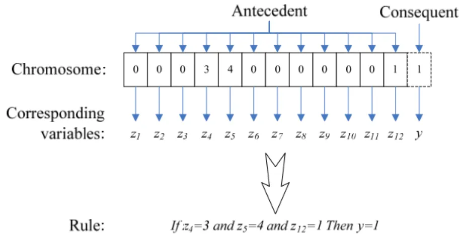
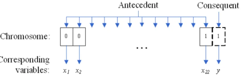
In the Michigan approach, each chromosome represents a candidate If-then rule. The conditions associated in the “if part” are termed as antecedent and those in the “then part” are named consequent. Besides, the antecedent part consists of at least one to at most twelve variables selected from Table 2 and the consequent part is composed by, of course, only one variable: liability degree of involved party. In general a rule is a knowledge representation of the form If A then C, where A is a set of parties satisfying the conjunction of predicting attribute values and C is a set of parties with the same predicted class. Thus, a typical rule i can be of the form:

Rule i: If z1=ai1 and z2=ai2 …and zj=aij … and z12=ai12 Then y=gi or of a shorter form:

Rule i: If Ai Then Ci.

where, aij is the categorical value of jth attribute variable in rule i. gi is the value of classification variable in rule i, which ranges from 1 to 5 to represent five degrees of liability. Ai and Ci, again, are the sets of parties satisfying the antecedent part and consequent part of rule i, respectively.

By encoding a rule as a chromosome, each gene is used to represent a corresponding variable. The length of a chromosome is set as 13 to represent twelve state variables in the antecedent part and one control variable in the consequent part. Each gene takes one of the categorical values of the corresponding variable. It is worthy of noting that the ranges of gene value may differ from each other since the range of corresponding variable is different. In addition, a gene in a rule antecedent is allowed to take a value of 0 to represent that its corresponding variable is not considered by the rule. If all genes in the antecedent part simultaneously take a value of 0 or the gene in the consequent part takes 0, then the whole rule is not included in the rule set.

Based on such an encoding method, a rule of “If speeding=”no” and alcoholic use=”no” and right-of- way=”yes”, then liability=”no responsibility” can be encoded as 0003400000011 as depicted in Fig. 1. The total number of potential rules equals to 6¯6¯6¯4¯5¯5¯4¯10¯8¯3¯13¯3¯5 =4,043,520,000, making the number of potential rule combinations reaches 24,043,520,000. Obviously, it is barely possible to compare all rule combinations by a total enumeration manner.

Fig. 1. Encoding methods of party-based Michigan model (GRM1)

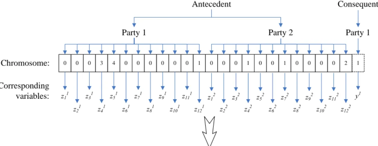
In the context of two-car crash accidents, it is interesting to compare the performance of the models which simultaneously consider the state variables of both parties involved or only consider that of one party alone. Therefore, two GRM models, namely GRM1 and GRM2, are proposed. The GRM1 is a party-based Michigan approach model which considers the state variables of one party alone to conclude the liability degree for the party as shown in Fig.1, while GRM2 is a case-based Michigan approach model which considers both parties involved simultaneously to conclude the liability degree of one party. Since the sum of liability degrees of two parties, party 1 and party 2,

(8)

involved in an accident are always equal to a constant, i.e. 6. For instance, of party 1 is judged as no responsibility for the accident, then party 2 must have to take full responsibility. The chromosome length of the GRM2 is 25 as depicted in Fig. 2.

0 z11 Party 1 Consequent 0 z21 0 z31 3 z41 4 z51 0 z61 0 z71 0 z81 0 z91 0 z101 0 z111 1 z121 1 y1

If z41=3 and z51=4 and z121=1 AND z42=1 and z72=1 and z122=2 Then y1=1 ( y2=5)

Chromosome:

Corresponding variables:

Rule:

Interpretation: If speeding of party 1=“no” and alcoholic use of party 1=“no” and right-of-way of party 1=“yes” AND speeding of party 2=“seriously speeding” and foresight of the accident of party 2=“yes” and right-of-way of party 1=“no” Then liability of party 1=“no responsibility” (implying that liability of party 2=“major responsibility”)

0 0 0 1 0 0 1 0 0 0 0 2 Antecedent Party 2 z12 z22 z32 z42 z52 z62 z72 z82 z92 z102 z112 z122 Party 1

Fig. 2. Encoding methods of case-based Michigan model (GRM2) (2) Pittsburgh approach

In contrast to the Michigan approach, the Pittsburgh approach simultaneously encodes all mined rules, a rule set, as a chromosome by simply extending the length of a chromosome to a multiple length of the Michigan approach’s chromosome of the number of rules. Therefore, the quality of the chromosome, i.e. fitness function, can straightforwardly represent the correctness rate of the rule set. Taking a preset number of rules (K)=20 for instance, the party-based encoding method (hereinafter, named as GRM3) can be depicted as Fig. 3. The length of chromosome equals to 13×20=260. Obviously, the case-based Pittsburgh approach model will result in a very lengthy chromosome, thus it is not considered in this paper. Since the situations that all antecedent genes or the consequent gene in a rule take a value of 0, then it indicates that the rule will not be selected. In other words, the number of mined rules must be less than or equal to the preset number of rules (K).

Fig. 3. Encoding methods of party-based Pittsburgh model (GRM3)

2.1.3.2 Performance indices

For the Michigan approach, the role of the fitness function is to evaluate the quality of the rule numerically. In doing so, three common factors to be taken into account are the coverage, the completeness and the confidence factor of the rule, respectively defined as follows. The coverage of the rule, i.e. the cases satisfied by the rule antecedent, is given by A, the cardinality of set A (the number of elements in set A). The completeness of the rule, i.e. the proportion of cases of the target

(9)

class covered by the rule, is given by A_IC /C . The confidence of the rule, i.e. the predictive accuracy, is given by A_IC /A (Freitas, 1999). Based upon these three factors, this paper uses the performance indices including predictive accuracy, comprehensibility and interestingness narrated as follows.

(1) Predictive accuracy

Two ways to measure the predictive accuracy, also called confidence, are found in literature (Ghosh and Nath, 2004, Dehuri and Mall, 2006, Dehuri et al., 2008):

A C A P(ℜ)= _I / ) (1) ) ~ ( ) ~ ( ~ ~ ) ( C A C A C A C A C A C A P I I I I I I + × + × = ℜ (2) where P(ℜ) is the predictive accuracy of rule ℜ. A is a set of cases or parties satisfying the rule antecedent. C is a set of cases or parties satisfying the rule consequent. is the intersection operator. ~A and ~C are complement sets of A and C, respectively.

I

A is the cardinality of set A. (2) Comprehensibility

Comprehensibility is used to measure the family size of the rule. The smaller the rule, the more comprehensible (specific) it is. There are several ways to measure comprehensibility (Fedelis, 2000, Ghosh and Nath, 2004, Dehuri and Mall, 2006, Dehuri et al., 2008) for example:

c c M N C(ℜ)=1− (ℜ)/ (3) ) ( ) (ℜ =M_c−N_c ℜ C (4) A N C(ℜ)= − (5) ) 1 log( / ) 1 log( ) ( k m k C ℜ = + + + (6) where is the comprehensibility of rule C(ℜ) ℜ. )N_c(ℜ is the number of conditions in the rule . is the number of at most conditions a rule can have. N is the number of total cases. m and

k are the number of attributes involved in the antecedent part and consequent part, respectively.

ℜ M_c

(3) Interestingness

The third criterion of the rules, called interestingness, is used to measure how surprising, useful or novel the rule is. Two simpler expressions of interestingness can be found in literature (Piatetsky-Shapiro, 1991, Ghosh and Nath, 2004) as follows:

N C A C A I(ℜ)= _I − / (7) ) 1 ( ) ( N C A C C A A C A I ℜ = I × I − − I (8) where is the interestingness of rule I(ℜ) ℜ. N is the total number of cases or parties.

2.1.3.3 Proposed fitness functions

(1) GRM1 and GRM2

Many studies consider rule mining as a multi-objective problem and employ evolutionary algorithms to mine the Pareto-optimal rules with respect to abovementioned three indices. However, in mining classification rules instead of association rules, a combination of Pareto-optimal rules

(10)

might not necessarily perform best on the whole. Besides, the conflict and redundancy among mined rules are seldom considered in the literature. High redundancy and conflict among rules will cause too many similar or conflicting rules being mined.

Based on this, this paper designs a two-stage process to select chromosomes (rules). In the first stage, a fitness function, a performance index with a combination of coverage ratio, predictive accuracy, and predictive error, is defined and used to rank the chromosomes, which can be expressed as: ) ~ ( i i i i i i i i _A C A A C A N A f = × I − I (10) where, fi is the performance index of the ith chromosome. The first term of right hand side is coverage ratio. The second term is the predictive accuracy rate. The third term is predictive error rate. The equation can be then simplified as:

N C A N C A f i i i i i ~ I I ₋ = (11) In the second stage, to avoid selecting similar or conflicting rules, two indices, redundancy index and conflicting index, are respectively defined and then both used to filter high redundant and conflicting chromosomes (rules). The redundancy index of rule i is defined as

} { max 1 1 j i j i i j i A A A A l U I − = = (12) where li is the redundancy index of the ith chromosome which has already been ranked in a descending order. The conflicting index of rule i is defined as

} if { max 1 1 j i j i j i i j i A A g g A A t U I ≠ = − = (13)

where ti is the redundancy index of the ith chromosome which has been ranked in a descending order. A_i_IA_jif g_i ≠g_j is the number of cases or parties satisfying both antecedent of rules i and

j which have different predicted classes.

To facilitate the filtering process according to li and ti, two thresholds, L and T, for redundancy and conflict have to be given. Thus, if a chromosome reaches either or , then it will be replaced by another randomly re-generated chromosome (newly re-born chromosome). These two given thresholds will then determine how many chromosomes will survive in each of generation. The higher the values of the thresholds are, the more chromosomes will be replaced. Of course, if too many chromosomes are replaced by randomly generated chromosomes, the competitive genetics can not be successfully preserved and a randomly searching mechanism will be resulted. Thus, the values of these two thresholds should be carefully examined. It is worthy of noting that the redundancy and conflicting indices are computed through a mutual comparison matter by only comparing with the chromosomes ranked in front.

L

l_i ≥ t_i ≥T

The evolutional process of GRM1 and GRM2 can be depicted in Fig. 4. As shown from the figure, after selection, crossover, and mutation, the survived chromosomes are first ranked according to their fitness value, and then filtered by their redundancy and conflicting indices. In the process all highly redundant and conflicting chromosomes will be replaced by randomly generated ones until the stopping condition (a given number of generations in this paper) reaches. However, in the final generation, all highly redundant and conflicting chromosomes will be deleted without replacement. The finally survived chromosomes are the optimal combination of rules.

(11)

L li≥ ti≥T

Fig. 4. Evolutional process of the GRM1 and GRM2 models

Even if the chromosomes have been filtered by redundancy and conflicting indices, it can not be avoided that two or more rules with different predicted classes might still be simultaneously fired by a sample. To synthesize the predicted class of more then one rules fired, we take an average value of predicted classes of all fired rules and round it to a nearest integer, which can be expressed as:

∑

∈ = F j j g F Int sg ( 1 ) (14)

where, G is the predicted class of the algorithm. Int(⋅) is a rounding operator, which rounds value in parenthesis to a nearest integer. F is a set of sequence numbers of fired rules. As such, the correctness rate of the model can be then computed as the number of correctly predicted cases or parties (that is, the predicted class equal to the target class) divided by total number of cases or parties. (2) GRM3 Since a chromosome of the GRM3 model (the party-based Pittsburgh approach) represents a combination of rules, the fitness function of a chromosome can be directly expressed as correctness rate. Correctness rate is defined as the number of correctly predicted parties divided by the total number of parties in training or validation. In the case of more than one rule fired, Eq.(14) is also used to synthesize the predicted classes of all fired rules. The reasons for not taking redundancy and conflicting indices into account are that the GRM3 aims to maximize the correctness rate under a preset number of rules (K), at optimality, the redundancy and conflicts among rules should be largely avoided. 2.1.3.4 Genetic operators Because the genes in our GRM models are not encoded binary, simple genetic algorithms (Goldberg, 1989) cannot be used. Instead, we employ the max-min-arithmetical crossover proposed by Herrera et al.(1998) and the non-uniform mutation proposed by Michalewicz (1992). A brief description is given below. (1) Max-min-arithmetical crossover Let Gwt ={ gw1t ,…, gwkt ,…, gwKt } and Gvt ={ gv1t ,…, gvkt ,…, gvKt }be two chromosomes selected for crossover, the following four offsprings will be generated: G1t+1 = aGwt + (1-a)Gvt (15)

G2t+1 = aGvt + (1-a)Gwt (16)

G3t+1 with g3kt+1=min{gwkt, gvkt} (17)

G4t+1 with g4kt+1=max{gwkt, gvkt} (18)

(12)

(2) Non-uniform mutation

Let Gt = { g1t ,…, gkt ,…, gKt } be a chromosome and the gene gkt be selected for mutation (the domain of gkt is [gkl, gku]), the value of gkt+1 after mutation can be computed as follows:

⎩ ⎨ ⎧ = − Δ − = − Δ + = + 1 ) , ( 0 ) , ( 1 b if g g t g b if g g t g g _l k t k t k t k u k t k t k 　　　　　　 (19) where b randomly takes a binary value of 0 or 1. The function Δ(t,z) returns a value in the range of [0, z] such that the probability of Δ( zt, ) approaches to 0 as t increases:

) 1 ( ) , (_t _z =_z −_r(1−t/T)h Δ ₍₂₀₎ where r is a random number in the interval [0,1], T is the maximum number of generations and h is a given constant. In Eq.(20), the value returned by Δ( zt, ) will gradually decrease as the evolution progresses.

2.1.4 Results

2.1.4.1 Parameter settings

The parameters of GAs are set as follows. Population size=100, crossover rate=0.9, a=0.3,

h=0.5, T=200. Redundancy index threshold (L) and conflicting index threshold (T) are set as 0.75

and 0.5, respectively. The number of generations is set as 200.

2.1.4.2 Comparisons

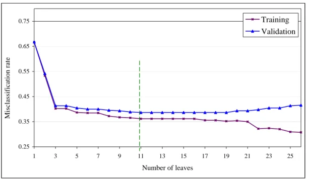
A k-fold (k=3 in this paper) cross-validation method is adopted for algorithm comparisons. A total of 537 accident cases (1,074 parties) are randomly and equally divided into three subsets, each of which contains 179 cases (358 parties). Each model is trained and validated three times separately. The average training and validation results of various algorithms are reported in Table 3. As noted from Table 3, GRM1 performs the best, both in training and validation, with correctness rates of 78.85% and 70.21%, respectively, followed by GRM2 with training and validation correctness rates of 74.34% and 69.33%, respectively. GRM3 performs the worst with training and validation correctness rates ranging from 69.20%~71.21% and 65.84%~67.55% under various preset numbers of rules, respectively. It is worthy of noting that the correctness rate of GRM3 does not increase monotonically as anticipated as the preset number of rules gets larger. It might be partly due to the searching space being exponentially increased as the preset number of rules gets larger, making the optimal combination of rules rather difficult to be mined. In terms of the number of rules mined, the GRM1 model selects the largest number of rules (34 rules), followed by 30 rules mined by GRM3 with K=35. Even under the limitation of at most 10 rules mined (GRM3 with

K=10), the correctness rates can still reach 69.20% in training and 66.46% in validation.

Table 3

The training and validation results of various GRM models

Correctness rate (%)

Models Maximum number

of rules allowed

Number of rules

mined Training Validation

GRM1 100 34 78.85 70.21 GRM2 100 28 74.34 69.33 10 10 69.20 66.46 15 15 69.60 66.15 20 20 70.00 67.08 25 24 69.47 65.84 30 28 69.23 66.87 GRM3 35 30 71.21 67.55

(13)

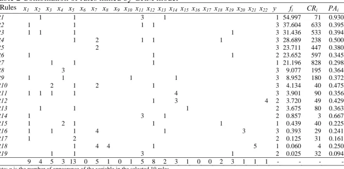
To get an in-depth investigation to the rules mined by the best performing model, GRM1, the fitness value, coverage ratio, predicted accuracy, redundancy index and conflicting index of a total of 34 mined rules are shown in Table 4. These rules are ranked according to fitness value fi in Eq.(11). Note that in terms of coverage ratio, R17 can cover the largest number of parties (46% of 1,074 parties, i.e. 494 parties), followed by R1 (43% of 1,074 parties, i.e. 462 parties). In contrast, R33 and R34 are customized to rather few parties with a low coverage ratio of 1%. In general, the more explanatory variables introduced into the antecedent of a rule, the lower the coverage ratio of the rule will be.

In terms of predicted accuracy, R19 and R21 perform the best with predicted accuracy of 91%, followed by R4 and R20 with predicted accuracy of 85%. R33 and R34 have the lowest predicted accuracy of 50%. In terms of redundancy index, R7 has the highest value of 72%, which is found to be highly overlapping with R2, followed by R4 of 65% overlapping with R2. Actually, both R7 and R4 are belonging to the family rules of R2. There are still many rules having no redundancy to their previous rules. In terms of conflicting, R23 performs the worst with conflicting index as high as 42%, which highly conflicts with R3, followed by R12 with conflicting value of 21% which conflicts with R8.

Also note that a total of 17 rules (the largest number) are mined of the predicted class of “no responsibility,” followed by six rules with the predicted class of “full responsibility.” Only two rules with the predicted class of “equal responsibility” are mined.

(14)

Table 4

Combination of rules mined by the GRM1 model

Rules Antecedent Consequent Fitness

value Coverage ratio Predicted accuracy Redundancy index Conflicting index Rule 1

If location=“straight road” and right-of-way=“yes” Then liability=“no” 0.28 0.43 0.83 0.00 0.00

Rule 2 If alcoholic use=“no” and relative direction=“opposing direction”

and right-of-way=“yes” Then liability=“no” 0.22 0.33 0.83 0.21 0.00

Rule 3

If relative direction=“same direction” and right-of-way=“no” Then liability=“full” 0.20 0.34 0.79 0.00 0.00

Rule 4 If type of vehicle=“passenger car” and alcoholic use=“no” and

relative direction=“opposing direction” and right-of-way =“yes” Then liability=“no” 0.16 0.22 0.85 0.65 0.00

Rule 5 If location=“straight road” and type of vehicle=“passenger car” and

speeding=“no” and right-of-way=“yes” Then liability=“no” 0.15 0.23 0.81 0.55 0.00

Rule 6 If location=“straight road” and foresight of the accident=“no” and

driver death =“no” and right-of-way =“yes” Then liability=“no” 0.14 0.22 0.82 0.48 0.00

Rule 7 If speeding=“no” and relative direction=“opposing direction” and

right-of-way=“yes” Then liability=“no” 0.11 0.37 0.65 0.72 0.00

Rule 8 If relative direction =“right adjacent direction” and

right-of-way=“yes” Then liability=“minor” 0.11 0.27 0.71 0.17 0.00

Rule 9

If relative direction=“left adjacent direction” and right-of-way=“no” Then liability=“major” 0.10 0.28 0.69 0.00 0.00

Rule 10

If relative direction=“opposing direction” and right-of-way=“no” Then liability=“full” 0.09 0.35 0.63 0.00 0.00

Rule 11

If location=“unsignalized intersection” and right-of-way=“yes” Then liability=“minor” 0.09 0.34 0.63 0.25 0.00

Rule 12 If location=“signalized intersection” and speeding=“no” and driver

death =“no” and right-of-way =“yes” Then liability=“no” 0.09 0.19 0.73 0.32 0.21

Rule 13 If type of vehicle=“passenger car” and foresight of the accident=“not

clear” and right-of-way =“no” Then liability=“full” 0.08 0.28 0.65 0.12 0.08

Rule 14 If speeding=“no” and alcoholic use=“no” and relative

direction=“opposing direction” and driver death =“no” and

right-of-way =“yes”

Then liability=“no” 0.08 0.27 0.66 0.52 0.00

Rule 15 If speeding=“seriously” and relative direction=“opposing direction”

(15)

Rule 16

If location=“unsignalized intersection” and right-of-way=“no” Then liability=“major” 0.07 0.36 0.59 0.00 0.00

Rule 17 If speeding=“no” and foresight of the accident=“yes” and

Rule 18 If alcoholic use=“no” and foresight of the accident=“not clear” and

right-of-way =“yes” Then liability=“no” 0.06 0.29 0.60 0.25 0.00

Rule 19 If foresight of the accident=“no” and relative direction=“same

direction” and right-of-way =“yes” Then liability=“no” 0.06 0.07 0.91 0.00 0.00

Rule 20 If location=“straight road” and type of vehicle =“truck” and driver

death=“no” and right-of-way =“yes” Then liability=“no” 0.06 0.08 0.85 0.21 0.00

Rule 21 If location=“straight road” and type of vehicle =“light truck” and

right-of-way =“no” Then liability=“full” 0.05 0.07 0.91 0.00 0.00

Rule 22 If foresight of the accident=“not clear” and driver death=“no” and

Rule 23 If speeding =“no” and foresight of the accident=“no” and driver

death=“no” and right-of-way =“no” Then liability=“major” 0.03 0.33 0.55 0.57 0.42

Rule 24 If location=“flashlight intersection” and type of vehicle =“passenger

car” and relative direction=“same direction” and right-of-way =“yes”Then liability=“minor” 0.03 0.06 0.78 0.17 0.08

Rule 25 If type of vehicle=“light truck” and relative direction=“same

direction” and driver death =“no” and right-of-way =“yes” Then liability=“no” 0.03 0.06 0.74 0.39 0.00

Rule 26 If type of vehicle=“passenger car” and foresight of the

accident=“no” and right-of-way=“yes” Then liability=“no” 0.02 0.41 0.53 0.55 0.00

Rule 27 If foresight of the accident=“no” and relative direction=“left adjacent

direction” and right-of-way =“yes” Then liability=“minor” 0.02 0.05 0.69 0.05 0.03

Rule 28 If location=“straight road” and type of vehicle=“light truck” and

speeding=“no” and right-of-way =“no” Then liability=“minor” 0.02 0.16 0.56 0.00 0.00

Rule 29 If type of vehicle=“truck” and alcoholic use=“no” and relative

direction=“opposing direction” and right-of-way =“no” Then liability=“full” 0.01 0.03 0.70 0.21 0.00

Rule 30 If speeding =“seriously” and foresight of the accident=“yes” and

right-of-way =“yes” Then liability=“equal” 0.01 0.04 0.61 0.07 0.05

Rule 31 If type of vehicle =“passenger car” and foresight of the

accident=“no” and relative direction=“opposing direction” and right-of-way =“yes”

Then liability=“no” 0.01 0.05 0.56 0.11 0.00

Rule 32 If type of vehicle=“light truck” and foresight of the accident=“yes”

(16)

Rule 33 If relative direction=“same direction” and driver death=“yes” and

Rule 34 If location=“straight road” and type of vehicle=“truck” and

(17)

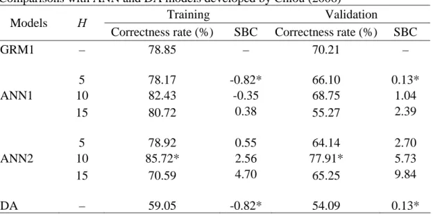
Table 5 further compares the results from our proposed GRM1 model and from the ANN and DA models developed by Chiou (2006). In terms of correctness rate, ANN2 model (case-based) with 10 hidden neurons performs the best both in training and validation, followed by ANN1 model (party-based) with 10 hidden neurons, ANN1 (12-10-1), in training and the proposed GRM1 model in validation. The DA model still performs the worst. In consideration of model’s accuracy and complexity, Chiou (2006) finally selected ANN1 (12-5-1) as the best performed model according to SBC. However, it is hard to identify the number of parameters of genetic algorithms, thus SBC of the proposed GRM1 model is not computed. Nonetheless, it is worth noting that the correctness rates of training and validation of GRM1 model are both higher than ANN1 (12-5-1).

Table 5

Comparisons with ANN and DA models developed by Chiou (2006)

Training Validation

Models H

Correctness rate (%) SBC Correctness rate (%) SBC

GRM1 – 78.85 – 70.21 – 5 78.17 -0.82* 66.10 0.13* ANN1 10 82.43 -0.35 68.75 1.04 15 80.72 0.38 55.27 2.39 5 78.92 0.55 64.14 2.70 ANN2 10 85.72* 2.56 77.91* 5.73 15 70.59 4.70 65.25 9.84 DA – 59.05 -0.82* 54.09 0.13*

Note: SBC stands for Schwarz’s Bayesian Criterion. SBC=ln(MSE)+Pln(N)/N, where, MSE is mean squared error, P is the number of parameters. * indicates the best performing model in terms of corresponding criterion. H is the number of hidden neurons.

To gain in-depth investigation on the validation results of different models, the number of parties with degrees of liabilities predicted by DA, ANN1 (12-5-1), and GRM 1 are reported in Tables 6~8, respectively. Note that the DA model has the highest correctness rate of 66.90% for the category of real y = 5 and the lowest correctness rate of 5.00% for the category of real y = 3, suggesting that DA model performs rather poorly in the cases of equal liability. In contrast, ANN1 (12-5-1) model can achieve over 60% of correctness rate almost for all categories, except for the category of real y = 4. Besides, the degrees of liabilities even incorrectly predicted by ANN do not deviate over one degree from their real ones; except for a total of 19 (1.77%) parties which are deviated two degrees. The proposed GRM1 model can accurately predict the liability for the categories of y= 1 or 5 with correctness rates of 92.25% and 91.90%. Even for the categories of y= 2 or 4, the proposed model can still reach about 60% of correctness rate. However, the proposed model is unable to predict the liability for the category of y = 3. The correctness rate of that category is only 8.33%. Nonetheless, the degrees of liabilities, even incorrectly predicted by GRM, do not deviate over one degree from their real ones; except for a total of 3 parties which are deviated two degrees. Besides, the proposed GRM1 model tends to produce much more predicted classes at both extremes: y=1 or y=5 than at the middle, i.e. y=3.

(18)

Table 6

The number of parties with degrees of liabilities predicted by the DA model Predicted y Real y 1 2 3 4 5 Total 1 157 (55.28) 98 (34.51) 20 (7.04) 9 (3.17) 0 (0.00) 284 (100.00) 2 86 (38.57) 125 (56.05) 0 (0.00) 11 (4.93) 1 (0.45) 223 (100.00) 3 18 (30.00) 12 (20.00) 3 (5.00) 12 (20.00) 15 (25.00) 60 (100.00) 4 2 (0.90) 36 (16.14) 0 (0.00) 106 (47.53) 79 (35.43) 223 (100.00) 5 0 (0.00) 3 (1.06) 30 (10.56) 61 (21.48) 190 (66.90) 284 (100.00) Total 263 274 53 199 285 1074

Note: The percentages are given in the parentheses.

Table 7

The number of parties with degrees of liabilities predicted by the ANN1 model Predicted y Real y 1 2 3 4 5 Total 1 202 (71.13) 69 (24.30) 13 (4.58) 0 (0.00) 0 (0.00) 284 (100.00) 2 54 (24.22) 139 (62.33) 30 (13.45) 0 (0.00) 0 (0.00) 223 (100.00) 3 0 (0.00) 11 (18.33) 41 (68.33) 8 (13.33) 0 (0.00) 60 (100.00) 4 0 (0.00) 4 (1.79) 44 (19.73) 107 (47.98) 68 (30.49) 223 (100.00) 5 0 (0.00) 0 (0.00) 2 (0.70) 61 (21.48) 221 (77.82) 284 (100.00) Total 256 223 130 176 289 1074

Note: The percentages are given in the parentheses.

Table 8

The number of parties with degrees of liabilities predicted by the GRM1 model Predicted y Real y 1 2 3 4 5 Total 1 262 (92.25) 20 (7.04) 2 (0.71) 0 (0.00) 0 (0.00) 284 (100.00) 2 88 (39.46) 133 (59.64) 2 (0.90) 0 (0.00) 0 (0.00) 223 (100.00) 3 0 (0.00) 24 (40.00) 5 (8.33) 31 (51.67) 0 (0.00) 60 (100.00) 4 0 (0.00) 3 (1.35) 0 (0.00) 137 (61.43) 83 (37.22) 223 (100.00) 5 0 (0.00) 0 (0.00) 0 (0.00) 23 (8.10) 261 (91.90) 284 (100.00) Total 350 180 9 191 344 1074

Note: The percentages are given in the parentheses. 2.1.4.3 Discussions

The proposed GRM1 models may not exhibit remarkably higher correctness rate than all of ANN models developed by Chiou (2006); however, the proposed models can generate meaningful rules for further examination and demonstration, making the GRM-based expert system much more understandable than the black-box ANN approach. Consequently, decision makers might feel more confident in using this GRM-based expert system. Besides, with rules mined, the accident appraisal knowledge can be clearly displayed and used to train junior members. And, it also offers a post-optimization mechanism which can further fine-tune the mining rules by interviewing the accident appraisal experts.

To further investigate the rules mined in Table 4, only eight out of twelve explanatory variables appeared in at least one rule, including location, type of vehicle, speeding, alcoholic use, foresight of the accident, relative direction, driver death, and right-of-way. Particularly, all of the rules introduce the variable of right-of-way, explaining its importance in accident appraisal. Furthermore, most of the rules with right-of-way=“yes” will also lead to the consequents of liability=“no responsibility” or “minor responsibility.” In contrast, the rules with right-of-way=“no”, then the liabilities are most likely to be “major responsibility” or “full responsibility.” As such, one may

(19)

argue that the accident appraisal can be conducted solely depending upon right-of-way. However, in doing so, the correctness rate is only 48.65%, which is even lower than that of the DA model.

Unlike the right-of-way being a decisive factor, some variables appearing in the rules are more likely to act like an environmental factor, such as location and relative direction, to determine whether the accident situation is clear or ambiguous. In a relatively clearer situation, such as location=“straight road,” or relative direction=“same direction” or “opposing direction”, the liability degree tends to be overwhelmingly assessed as either “no responsibility” or “full responsibility” solely depending on right-of-way, such as the rules of R1, R2, R3, R5, and R6 etc. In contrast, in a relatively more ambiguous situation, such as location=“unsignalized intersection” or “flashlight intersection” or relative direction=“left adjacent direction” or “right adjacent direction,” then the liability degree are more conservatively assessed as “minor responsibility” and “major responsibility,” such as the rules of R8, R9, R11, and R16 etc.

On the other hand, some variables operate like an incremental factor to further raise or alleviate the liability degree accompanying with the ownership of right-of-way. These variables are violation variables, including speeding and alcoholic use. Taking R30 for instance, the liability degree is suggested as “equal responsibility,” when the party was seriously speeding even with the ownership of right-of-way.

High redundancy relationship can still be found among rules mined. Taking R4 for instance, it belongs to the family rules of R2. It is said that R4 is more specific than R2 by further specifying the type of vehicle. Due to the high redundancy between these two rules, deleting any one of them may not seriously deteriorate the correctness rate, if the number of rules is strictly limited.

In comparing the degree of liability predicted with different models, the proposed GRM model performs worse in predicting the category of liability=“equal responsibility,” because very few related rules (with consequent part of liability=“equal”) have been mined. Two reasons could be identified. First, the number of parties with liability=“equal responsibility” in the dataset is only approximately one fourth of other degrees, thus it is difficult to learn representative rules from limited parties. Second, since the right-of-way is very decisive to liability assessment, all predicted results are clearly divided into two distinct categories: no (minor) and full (major) degrees, leaving no much room for middle degree.

Four explanatory variables: type of road, direction, crash spot, and LAC, are not included in any rule of a total of 34 rules. It can be explained that they are not key factors to the accident appraisal. However, it might also be possible that these variables are categorized into too many classes, e.g. crash spot (8 classes) and LAC (12 classes). In general, GRM tends not to choose a variable with too many classes, because the number of cases or parties belonging to each class will be small and lower the coverage ratio. Thus, it would be very helpful to collect more cases with equal responsibility for training or to approximately merge some classes into fewer categories.

2.1.5 Concluding remarks

This paper employs genetic rule mining (RGM) to develop accident appraisal expert systems by discovering knowledge from historical appraisal cases, which can not only accurately predict the liability degrees of involved parties but also demonstrate comprehensive appraisal rules and further provide the flexibility of post-adjustment of mined rules. Three GRM models based on the Michigan approach (GRM1 and GRM2) and the Pittsburgh approach (GRM3) have been developed in this study. To effectively mine rules based on the Michigan approach, a novel two-stage rule selection procedure is proposed. The first stage is to rank the chromosomes survived from selection, crossover, and mutation operations according to a fitness function composed by coverage ratio, predicted accuracy and predicted error. The second stage is then to filter the ranked chromosomes depending on whether their redundancy and conflicting indices are larger than the preset thresholds.

For training and validating the proposed three models, a total of 537 two-car crash accident cases (1074 parties) are randomly and equally divided into three subsets, each of which contains

(20)

179 cases (358 parties). Each model is trained and validated three times separately. The results show that the GRM1 model, party-based Michigan approach, performs the best with training and validation correctness rates of 78.85% and 70.21%, respectively. Comparisons with the ANN1, ANN2, and DA models proposed by Chiou (2006) also show that the proposed GRM1 model can achieve the accuracy level of ANN models, but more importantly, the GRM1 model can generate a comprehensive combination of rules. Through an in-depth investigation on a total of 34 rules mined by GRM1 model, some underlying accident appraisal knowledge can be extracted. First, right-of-way is found to be a decisive factor which not only shows in every rule mined but also determines most of the liability degree as two distinct categories: no (or minor) responsibility vs. full (or major) responsibility depending upon which party owns the right-of-way. Second, some environmental variables, such as location and relative direction, appear in rules to determine how clear the accident situation was, which then lead the liability degree to be either an overwhelming result: no responsibility vs. full responsibility or to be a conservative result: minor responsibility vs. major responsibility. Third, some violation variables, such as speeding or alcohol use, are then used to add or relieve liability degree which has been assessed based on other facts.

Several directions can be identified for future studies. First, the encoding method for the Pittsburgh approach proposed in this paper is rather lengthy, as a result that the case-based Pittsburgh model can not be considered. A more compact and efficient encoding method for Pittsburgh approach deserves further studies. Besides, the proposed two-stage chromosome ranking and filtering procedure of the Michigan approach is somewhat inefficient because of ranking process involved. A more efficient procedure deserves further explorations. Although the proposed GRM1 model can accurately predict the liability degrees of y = 1 or 5 with correctness rate over 90%, and can still predict at a satisfactory correctness rate for the liability degrees of y = 2 or 4 (about 60%), it performs rather poorly in predicting the liability degree of y = 3. Since the number of training samples with such a liability degree is only one-fourth of samples with other degrees, we believe that it can further enhance the predictive capability of proposed models by collecting more such accident appraisal cases. It is also essential to fine-tune the rules mined by interviewing senior accident appraisal experts through an interactive manner. Last but not least, the fact that some variables do not appear in any rule might partly contribute to their values being classified into too many categories, leading to a rather small share of cases or parties covered in each category. To properly merge their categories without losing too much meaningful knowledge is also worthy of exploration.

2.2 事故分析 2.2.1 Introduction

Crash data analysis can be carried out by two main approaches: collective approach and individual approach (Abdel-Aty and Pande, 2007). The collective approach is characterized by crash frequency modeling. Frequency of crashes is aggregated over specific time periods (months or years) and locations (segments or intersections). Most of these studies attempt to explore the relationship between crash counts and explanatory variables, such as roadway geometry, traffic control facilities, traffic conditions, and so on by using Poisson or Negative Binomial regression models (e.g. Poch and Mannering, 1996; Milton and Mannering, 1998; Ivan et al., 1999, Abdel-Aty and Radwan, 2000, Greibe, 2003, Abdel-Aty and Pande, 2007, Wong et al., 2007). For the collective approach, however, individual contributing factors to the crash (e.g., driver demographics, driver behaviors, vehicle types) are not considered and factors affecting the crash severity cannot be identified either. Therefore, some studies employed individual approach to crash data analysis. The individual approach is characterized by each individual crash case. The main focus of these studies was to associate the crash severity with driver, vehicle and roadway factors by using ordered probit/logit model or logistic regression (e.g., Shanker, et al., 1996; Shanker and Mannering, 1996; Dissanayake

(21)

et al., 2002, Al-Ghamdi, 2002; Delen, et al., 2002; Tay and Rifaat, 2007; Sze and Wong, 2007).

Although statistic models are the most commonly used methods in the context of crash data analysis either collectively or individually, most of them have their own assumptions and complexity in model estimation and interpretation. Once the assumptions were violated, the model could lead to erroneous estimation results. Especially for the individual approach, most of the variables explaining the individual crashes are categorical, such as driver gender, road type, lighting condition, violation, weather condition, and severity degree, etc. It is difficult to develop parametric statistical models based upon such categorical data. Therefore, a number of distribution-free methods, particularly for dealing with classification and prediction problems such as decision tree (Chang and Chen, 2005; Chang and Wang, 2006) and artificial neural network (Chiou, 2006; Delen

et al., 2006), were adopted. However, two gaps still remain. First, the interpretations of

classification results with such methods are weak. The knowledge lying in the crash data cannot be fully discovered, because artificial neural network is a black-box characterized method and the prediction error of decision tree is usually high. Second, most of statistical methods only provide calibrated parameters with significance tests, which are then used to examine the effects of the corresponding variables on crash counts or crash severity. The interrelationship among explanatory factors cannot be examined in details. According to “error chain theory,” a crash is often caused by a series of errors, not solely by a single factor. As such, mining the explanatory rules is deemed necessary for crash data analysis.

Rule mining, also known as rule generation, rule recovery, or classification/association rule mining, is one of data mining techniques intended to mine for knowledge from available databases and toward decision support. Rule mining is naturally modeled as multi-objective problems with three criteria: (1) predictive accuracy, (2) comprehensibility, and (3) interestingness (Freitas, 1999; Ghosh and Nath, 2004). To automatically search for the optimal combination of rules from a considerable number of potential rules, genetic algorithms (GAs) are perhaps the most commonly used method. By employing GAs to learn of rules is named as genetic mining rule (GMR) (e.g. Freitas, 1999; Shin and Lee, 2002; Ghosh and Nath, 2004; Dehuri and Mall, 2006; Chen and Hsu, 2006). The performances of rule mining algorithms have been proven and applied in many fields. Thus, this paper aims to develop GMR model that can determine the optimal combination of appraisal rules to achieve the following goals: (1) to discover the key rules that determine the combination of contributing factors’ level to crash severity; (2) to provide the possibility of post-adjustment (fine-tune) of the rules mined; (3) to accurately predict the crash severity. Previous relevant studies have seldom considered the problems of conflicts and redundancy among the rules mined, our proposed GMR model will account for the conflicts and redundancy, in addition to conventional objectives: coverage ratio and predictive accuracy.

2.2.2 Data

The crash data was collected from 2003-2007 National Traffic Accident Investigation Reports compiled by National Police Agency, Taiwan. Each accident investigation report has been digitized and maintained in the database from which detailed individual crash data of freeway accidents are obtained. Each individual crash data include detailed information regarding injury severity of each involved individual, time of accident, driver demographics (age, gender, driver sobriety), involved vehicle types, roadway geometry, traffic control condition, weather condition (clear, rain, fog), pavement conditions (wet, dry), lighting condition, vehicle actions (moving straight, right-turn, left-turn, lane-change), and collision types.

There are 52,117 crash cases occurring on Taiwan freeways from 2003 to 2007. The injury severity of crashes is determined according to the injury degree of the worst-injured victims in the accident.

(22)

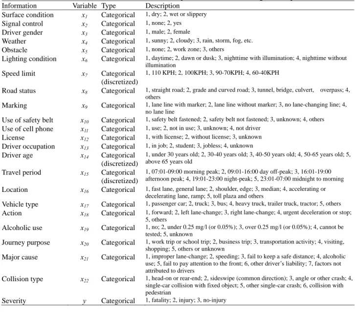
After screening out incomplete police investigation report, a total of 45,744 crashes are used for this study. Table 1 presents the definition and description of potential explanatory variables to crash severity.

Table 1 Crash data summarized from police accident investigation reports

Information Variable Type Description

Surface condition x1 Categorical 1, dry; 2, wet or slippery

Signal control x2 Categorical 1, none; 2, yes

Driver gender x3 Categorical 1, male; 2, female

Weather x4 Categorical 1, sunny; 2, cloudy; 3, rain, storm, fog, etc.

Obstacle x5 Categorical 1, none; 2, work zone; 3, others

Lighting condition x6 Categorical 1, daytime; 2, dawn or dusk; 3, nighttime with illumination; 4, nighttime without illumination

Speed limit x7 Categorical

(discretized)

1, 110 KPH; 2, 100KPH; 3, 90-70KPH; 4, 60-40KPH

Road status x8 Categorical 1, straight road; 2, grade and curved road; 3, tunnel, bridge, culvert, overpass; 4, others

Marking x9 Categorical 1, lane line with marker; 2, lane line without marker; 3, no lane-changing line; 4, no lane line

Use of safety belt x10 Categorical 1, safety belt fastened; 2, safety belt not fastened; 3, unknown; 4, others

Use of cell phone x11 Categorical 1, use; 2, not in use; 3, unknown; 4, not driver

License x12 Categorical 1, with license; 2, without license; 3, unknown

Driver occupation x13 Categorical 1, in job; 2, student; 3, jobless; 4, unknown

Driver age x14 Categorical

(discretized)

1, under 30 years old; 2, 30-40 years old; 3, 40-50 years old; 4, 50-65 years old; 5, above 65 years old

Travel period x15 Categorical

(discretized)

1, 07:01-09:00 morning peak; 2, 09:01-16:00 day off-peak; 3, 16:01-19:00 afternoon peak; 4, 19:01-23:00 night-peak; 5, 23:01-07:00 midnight to morning

Location x16 Categorical 1, fast lane, general lane; 2, shoulder, edge; 3, median; 4, accelerating or decelerating lane, ramp; 5, toll plaza and others

Vehicle type x17 Categorical 1, passenger car; 2, truck; 3, bus; 4, heavy truck, trailer truck, tractor; 5, others

Action x18 Categorical 1, forward; 2, left lane-change; 3, right lane-change; 4, urgent deceleration or stop; 5, others

Alcoholic use x19 Categorical 1, no; 2, under 0.25 mg/l (or 0.05%); 3, over 0.25 mg/l (or 0.05%); 4, cannot be tested; 5, unknown

Journey purpose x20 Categorical 1, work trip or school trip; 2, business trip; 3, transportation activity; 4, visiting, shopping; 5, others or unknown

Major cause x21 Categorical 1, improper lane-change; 2, speeding; 3, fail to keep a safe distance; 4, alcoholic use; 5, fail to pay attention to the front; 6, other driver’s liability; 7, factors not attributed to drivers

Collision type x22 Categorical 1, head-on or rear-end; 2, sideswipe (common direction); 3, angle or other crash; 4, single-car collision with fixed object; 5, other single-car crash; 6, collision with pedestrian

Severity y Categorical 1, fatality; 2, injury; 3, no-injury

In Taiwan, crash severity in police investigation report is classified into three degrees: A1 (fatal crash), A2 (injury crash), and A3 (non-injury crash). The numbers of cases for these three degrees of crash severity are 494, 4,073, and 41,177, respectively—an uneven distribution commonly seen in the context of crash analysis. To avoid misleading results caused by sample disproportionate problem, A2 and A3 crash cases are randomly re-selected to the same number of A1 crash cases (494), thus making a total of 1,482 crash cases for our analysis. Furthermore, 70% of these 1,482 crash cases are randomly chosen for training (i.e., 1,037 cases) and the remaining 445 cases are used for model validation. χ2-test is performed and the result shows that severity distributions between training and validation datasets do not significantly differ.

2.2.3 Genetic rule mining

Genetic rule mining (GMR), which can automatically learn of comprehensive rules from available dataset and toward decision support, has been shown as a useful tool in accident analysis (Clarke et