啁啾式多層堆疊量子點雷射之特性暨其適用於光學同調斷層掃描系統之可行性分析研究

國立交通大學

電子工程系 電子研究所碩士班

碩士論文

啁啾式多層堆疊量子點雷射之特性

暨其適用於光學同調斷層掃描系統

之可行性分析研究

Characterization of

chirped-multilayer quantum dot laser and

feasibility study of its application on

Optical Coherence Tomography

研 究 生：黃俊仁

指導教授：林國瑞 教授

啁啾式多層堆疊量子點雷射之特性暨

其適用於光學同調斷層掃描系統之可行性分析研究 Characterization of chirped-multilayer quantum dot laser and

feasibility study of its application on Optical Coherence Tomography

研 究 生：黃俊仁 Student ：Chun-Jen Huang 指導教授：林國瑞 Advisor ：Gray Lin

國 立 交 通 大 學

電 子 工 程 系 電 子 研 究 所 碩 士 論 文

A Thesis

Submitted to Department of Electronics Engineering and Institute of Electronics College of Electrical and Computer Engineering

National Chiao Tung University In partial Fulfillment of the Requirements

For Degree of Master

In

Electronics Engineering

September 2009

Hsinchu, Taiwan, Republic of China

啁啾式多層堆疊量子點雷射之特性暨 其適用於光學同調斷層掃描系統之可行性分析研究 學生：黃俊仁 指導教授：林國瑞 國立交通大學 電子工程學系 電子研究所碩士班 摘 要 本篇論文主要是計對自行設計之啁啾式多層堆疊量子點寬頻雷射的同調性 暨其是否適用於生醫領域上在近年來蓬勃發展的光學同調斷層掃描術(OCT)來做 探討。為了定量寬頻光源的同調長度，我們架設了一套光纖式、並以程式自動控 制的促動器來調整光程差的 Mach-Zehnder 式干涉儀，並搭配一張高速數位器卡 整合成一套同調長度量測系統。為了驗證該量測系統的準確性，我們也用理論來 數學模擬了頻譜形式較為簡單的雷射，並與之和實驗結果相比較。 為了提供 OCT 系統更高解析度的光源，我們嘗試設計了一種多層堆疊結構的 量子點雷射(chirped- multilayer quantum dot laser diode, CMQD LD)，期望 利用其基態與激發態同時雷射的特性得到高輸出功率的寬頻光源。我們藉有系統 的量測來觀察該雷射的表現，包括其同調性，並發現當其操作於高電流時，於高 解析度 0.1 nm 的量測條件下，單一量子態的發光頻譜寬度可達到 29 nm，且當 中不存在任何 3dB 凹陷，而該頻譜中心位在 1270 nm，我們預估其同調長度可落 在 50 μm 以內。由於縱向模態的存在，我們提出量測干涉圖將是用來評斷一個“寬 頻”雷射是否合適於 OCT 系統應用的一個較直接且實際的方式。另外，於干涉圖 中光程差為零的主峰，其半高寬可視為用來檢視雷射寬頻程度的重要依據。最 後，我們也將提供 CMQD LD 在未來可以更適合做為 OCT 光源的設計思維。

Characterization of chirped-multilayer quantum dot laser and feasibility study of its application on

Optical Coherence Tomography

Student: Chun-Jen Huang Advisors: Dr. Gray Lin

Department of Electronics Engineering & Institute of Electronics Engineering National Chiao Tung University

Abstract

This thesis will focus on discussing the coherence of chirped multilayer quantum dot (CMQD) laser and feasibility study of its application on optical coherence tomography (OCT). To acquire the coherence information of CMQD, we have set up a fiber-based and delay-tunable Mach-Zehnder interferometer. The accuracy of measurement has been confirmed by mathematical simulation on commercial lasers.

To achieve an OCT light source with higher axial resolution, we have specially designed a chirped multilayer (N=10) quantum dot laser. The measurement of laser characteristics of CMQD was demonstrated, including interferograms. An extremely broad spectrum of 29 nm without any 3dB dip was achieved. It centered at 1270 nm and was expected to have a coherence length less than 50 μm. Due to the longitudinal modes, we conclude that measuring interferogram is a more direct and more practical way to decide if a “broad spectrum” laser is suitable or not for OCT application. Furthermore, the FWHM of the main peak in an interferogram could be viewed as an indicator for judging the broadness of the spectrum for a broadband laser. Finally, suggestions will be provided in order to improve the performance of CMQD.

致 謝

碩班生涯兩年，說長不長，說短不短，轉晃眼就這樣過去，回首 過往，我想這會是人生中最精華的一段。 有幸進到這個同時充滿活力與溫馨的實驗室，為我的研究生涯增 添不少色彩。感謝 MBE 實驗室裡的總舵手---李建平老師，嚴謹的研 究氣氛、完善的實驗設備、學術討論中給予的關鍵性指引以及令人振 奮的鼓舞，無疑地是我個人在研究之路上動力來源，將是我未來努力 朝向的目標。謝謝林聖迪老師，清晰的思路與時常地不吝叮嚀總提醒 了自己可以改進、努力的地方，透徹的理解力與隨時保持對未知事物 的積極求知慾，是我理想中的學習模範。感謝我的指導老師---林國 瑞老師，針對專業領域地廣泛訓練與實驗上不吝地給予實質上協助， 因此培養了自主學習和從錯誤中成長的學習態度，體驗到學習的真 諦，會是我一生受用無窮的寶貴資源。更謝謝大學時期的專題老師電 物系徐琅老師，當初對許多軟體的訓練讓我獲益良多。最後也鄭重感 謝台大光電所蔡孟燦學長、電物所羅志偉老師，無私地教導並提供經 驗上的珍貴資訊，是我在研究過程初期重要的引導者。 在碩士生涯初期得到不少應具備的實用基礎背景知識，感謝實驗 室中的大學長羅明城、凌鴻緒與林大鈞，曾一同參與的馬拉松比賽會 是我難忘的回憶，不論是玩樂或是做研究，認真面對生命中每件事物 一直是我想要從中學習的。謝謝同是電物出身的潘建宏與蘇聖凱學 長，曾在長晶、光路調整與研究方向上給予建議，伴我走過了不少學 習中的瓶頸。感謝巫朝陽和林建宏學長，除了在程式及光學系統設計 上慷慨給予幫助，閒暇一起丟球的時光帶給我不少充電的機會。謝謝 同是電物的同屆夥伴 queena，同樣的背景與一路走來的相互扶持， 感受到大學以來的感情延續。感謝林博、賴大師、品維、韋智、小傅， 幾個實驗室同伴時常彼此分享並互相打氣，一起走過了不少低潮和艱 難的時光。最重要的，感謝旭傑學長、小豪、JackSu、歪哥、皓皓、 小微、小史，除了實驗上實質地給予協助、討論、分享，每天課後一

同用餐與定期出遊培養出共患難的感情，同時釋放了許多壓力，是我 能夠一路走到此重要的推手，我想我會永遠珍惜並保持這段得來不易 的情誼。 走出實驗室，仍然是在自己過去熟悉的交大，同樣留在新竹的電 物同伴也扮演了我碩士過程中重要的地位。謝謝大頭、達叔在自己低 潮時總是給我支持和鼓勵，不失為我的心靈導師。感謝古新安、小給 和同寢六年的室友彥緯，在自己焦頭爛額的非常時期仍願意播時間陪 我討論到凌晨並給予許多關鍵性的建議。謝謝小猴和牛奶願意幫我把 連自己都看不下去的爛英文做了校稿的動作。感謝 yes、tsao、堯堯、 大給，陪伴我走過許多不在實驗室的課餘時光，讓我都能以全新的面 貌來面對看似艱困的每一天。 經過了許久的努力，不斷地克服接踵而至的挑戰，最後要感謝 的，是默默在背後支持我的家人，爸、媽與兩個弟弟，比起給予的實 質幫助，不論何時何地給我在精神上的支持，心照不宣的體會和諒 解，使我在為自己奮鬥的同時能夠無後顧之憂，於此將這份畢業的喜 悅獻給我的家人，謝謝。

Contents

Abstract (Chinese) i

Abstract (English) ii

Acknowledgement iii

Contents v

Table Captions vii

Figure Captions viii

Chapter 1 Introduction

1.1 Optical Coherence Tomography (OCT) 1

1.1.1 Time-Domain OCT (TD-OCT) 4

1.1.2 Axial and Transverse Resolution of OCT 5

1.1.3 Other types of OCT 7

1.2 Broadband Emitter for OCT 8

1.2.1 Superluminescent Diode (SLD) 8

1.2.2 Femtosecond Laser 9

1.3 Overview of Semiconductor Quantum Dot Laser 10

Chapter 2 Theoretical Fundamentals

2.1 Coherence Theory 13

2.1.1 Temporal Coherence 13

2.1.2 Wiener-Khinchin Theorem 18

2.2 Semiconductor Quantum Dot 20

2.2.1 Ideal Quantum Systems 20

2.2.2 Structural Characteristics of Quantum Dots 22

2.2.3 Carrier Transition in Quantum Dots 23

2.3 Quantum Dot Laser 24

2.3.2 Optical Gain and Laser Threshold 26

2.3.3 Characteristics of a Quantum Dot Laser 27

Chapter 3 Experimental Techniques

3.1 Coherence Length Measurement 30

3.1.1 Experimental Setup 30

3.1.2 The Accuracy of Measurement 33

3.2 Characteristics of Laser Diode 38

3.2.1 Light - Current - Voltage Characteristic 38

3.2.2 Lasing Spectrum 39

3.2.3 Far Field Pattern 39

Chapter 4 Chirped-Multilayer Quantum Dot Laser

4.1 Introduction 41

4.2 Device Growth and Fabrication 42

4.3 Results and Discussion 44

4.3.1 Laser Characteristics 45 4.3.2 Gain-Current Analysis 47 4.3.3 Far-Field Pattern 49 4.3.4 Temperature Characteristics 51 4.3.5 Spectral Characteristics 52 4.3.6 Coherence 58

Chapter 5 Conclusions and Future Works

5.1 Conclusions of Present Studies 69

5.2 Suggestions for Future Works 70

Reference 72

Table Captions

Chapter 4

Table 4.1 All parameters of FFP for the 3μm-wide ridge and 2-mm-long CMQD LD with increasing current density. 49 Table 4.2 The list of corresponding peak wavelength and FWHM as

increasing injection levels for all devices. 55

Figure Captions

Chapter 1

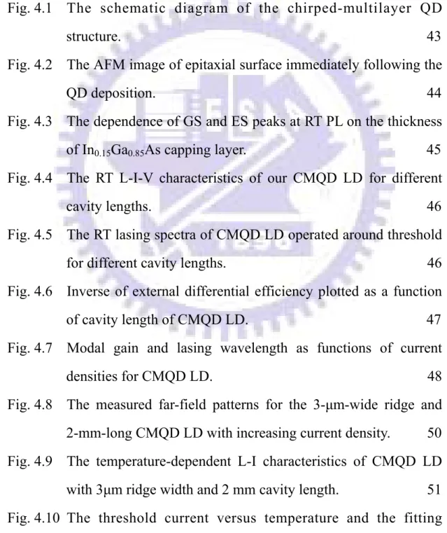
Fig. 1.1 A-scans measure the magnitude and echo time delay of backreflection or backscattering light. B-scans perform multiple axial scanning at different transverse position. By raster scanning a series of B-scan, C-scan or three-dimensional data set can be generated. 2

Fig. 1.2 OCT technology has typically axial resolution ranging from 1~15 um and imaging depth about 2 mm, which fills the gap between ultrasound and confocal microscopy. 3

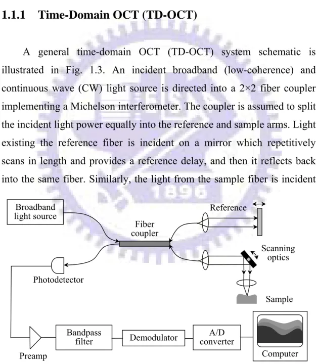
Fig. 1.3 A general time-domain OCT (TD-OCT) system schematic. 4

Fig. 1.4 The relationship between minimum spot size and depth of field. 7 Fig. 1.5 Optical bandwidth, interference signal and point spread

function using a typical SLD and a femtosecond Ti:Al2O3 laser. For ultra-high resolution OCT, a broadband femtosecond laser with spectrum bandwidth ~260 nm can achieve a free space axial resolution of 1.5 μm. 10

Chapter 2

Fig. 2.1 The Michelson interferometer. 14

Fig. 2.2 Graph of the self coherence function Γ(τ), and the contrast function K(τ) for light from completely coherent, completely incoherent and partially coherent light respectively. 17

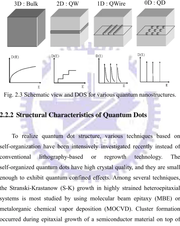
Fig. 2.3 S c h e m a t i c v i e w a n d D O S f o r v a r i o u s q u a n t u m nanostructures. 22 Fig. 2.4 Light propagation and its intensity in a round-trip cycle inside the Fabry-Perrot cavity. 26 Fig. 2.5 Schematic dependence of the optical gain on the current density for the ideal and real (self-organized) QDs. 29

Chapter 3

Fig. 3.1 The scheme of the coherence length measurement system. 30

Fig. 3.2 Photo of the fiber-based, computer-controlled MZI. 31 Fig. 3.3 The interface of the Labview control panel. 32

Fig. 3.4 (a) The power spectrum in linear scale, (b) IFFT of power spectrum, (c) IFFT of power spectrum in the measurable area (d) envelope detection on IFFT of power spectrum, (e) the experimental interferogram and (f) its detail for 1.31 F-P LD. 35 Fig. 3.5 (a) The power spectrum in linear scale, (b) IFFT of power

spectrum, (c) IFFT of power spectrum in the measurable area (d)envelope detection on IFFT of power spectrum, (e) the experimental interferogram and (f) its detail for 1.31 DFB LD. 36 Fig. 3.6 (a) The power spectrum in linear scale, (b) IFFT of power

spectrum, (c) IFFT of power spectrum in the measurable area (d) envelope detection on IFFT of power spectrum, (e) the experimental interferogram and (f) its detail of 1.55 DFB LD. 37 Fig. 3.7 The schematic diagram for the measurement of L-I-V

characteristic. 38 Fig. 3.8 The setup for the measurement of lasing spectrum. 39

Fig. 3.9 The setup for the measurement of FFP. 40

Chapter 4

Fig. 4.1 The schematic diagram of the chirped-multilayer QD structure. 43

Fig. 4.2 The AFM image of epitaxial surface immediately following the QD deposition. 44 Fig. 4.3 The dependence of GS and ES peaks at RT PL on the thickness of In0.15Ga0.85As capping layer. 45

Fig. 4.4 The RT L-I-V characteristics of our CMQD LD for different cavity lengths. 46

Fig. 4.5 The RT lasing spectra of CMQD LD operated around threshold for different cavity lengths. 46

Fig. 4.6 Inverse of external differential efficiency plotted as a function of cavity length of CMQD LD. 47

Fig. 4.7 Modal gain and lasing wavelength as functions of current densities for CMQD LD. 48

Fig. 4.8 The measured far-field patterns for the 3-μm-wide ridge and 2-mm-long CMQD LD with increasing current density. 50 Fig. 4.9 The temperature-dependent L-I characteristics of CMQD LD

with 3μm ridge width and 2 mm cavity length. 51 Fig. 4.10 The threshold current versus temperature and the fitting

curve. 52

Fig. 4.11 (a) ~ (h) The RT lasing spectrum operating from lasing threshold to well-above threshold current for CMQD LD with 3μm ridge width and different cavity lengths. 53 Fig. 4.12 The plot of peak wavelength versus current injection level for

each device. 56

Fig. 4.13 The evolution of spectrum at high injection level for CMQD. 57

Fig. 4.14 (a) ~ (e) The interferograms for CMQD LD with L ranging from 1.5 mm to 5 mm as increasing current injection and the linear-scale spectrum operating at 10*I_th. 59

Fig. 4.15 Simulation on interferogram of two adjacent Gaussian-like spectra with the same amplitude and FWHM. 65

Fig. 4.16 The main peak in interferograms as increasing current injection for 3-mm-long device of CMQD LD. 67

Fig. 4.17 The practical coherence length plotted as a function of current injection for CMQD LD. 68

Fig. 4.18 The FWHM of lasing spectra plotted as a function of injection current. 68

Chapter 1

Introduction

1.1 Optical Coherence Tomography (OCT)

Optical coherence tomography (OCT) is an emerging optical imaging and diagnostic technology in biomedical optics and medicine. OCT uses low-coherence interferometry to perform high resolution, cross-sectional and non-invasive imaging of the en-face internal microstructure in materials or biological tissues in a way that is analogous to ultrasonic pulse-echo imaging [1]. Tissue pathology can be imaged in

vivo and in real time with resolutions of 1~15 μm, about one to two

orders of magnitude finer than conventional ultrasound. The unique features of OCT make it a powerful imaging tool, which promises to enable many fundamental researches in many areas, especially in clinical applications.

OCT performs cross-sectional imaging by measuring the single axial magnitude and echo time delay of backscattered light (axial scan or A-scan) and then scanning the incident optical beam transversely, as shown in Fig. 1.1. The generated two-dimensional data set represents the optical backscattering in a cross-sectional plane through the sample. Images, or B-scans, can be displayed in false color or gray scale to visualize tissue morphology. Three-dimensional data sets can be generated by acquiring sequential cross-sectional images by scanning the incident optical beam in a raster pattern (C-scan). Three-dimensional OCT (3D-OCT) data contain comprehensive volumetric structural information and can be manipulated similar to magnetic resonance imaging (MRI) or computed tomography (CT).

Without invasion and the need to remove and process the specimens, OCT has advantage in particular clinical situation [2]. For example, applications include tissues such as the eye, coronary arteries or nerve, where biopsy is harmful or impossible. By means of coupling with catheter, endoscope or other needle delivery devices, OCT gradually performs to have impact on many clinical areas ranging from gastrointestinal tracts to other internal medicine.

To understand what role that OCT plays in the biomedical imaging method, it’s helpful to compare it with other conventional imaging technology. OCT imaging is analogous to ultrasound imaging except that it uses light instead of sound. Both the resolution and the penetration depth of ultrasound imaging depend on the frequency of sound wave

A scan B scan C scan

Axial (Z) scanning Axial (Z) scanning Transverse (X) scanning

Axial (X) scanning XY scanning

Fig. 1.1 A-scans measure the magnitude and echo time delay of backreflection or backscattering light. B-scans perform multiple axial scanning at different transverse position. By raster scanning a series of B-scan, C-scan or three-dimensional data set can be generated.

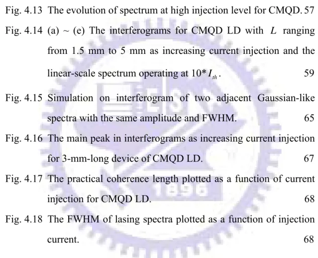
(3~40MHz) it uses [3]. High frequency ultrasound has been developed to achieve as high resolution as 15 μm with frequencies of ~100MHz. However, significant attenuation of the sound wave may occur with propagation and the imaging depths will be limited to only a few millimeters in such high frequencies. Microscopy and confocal microscopy are examples of high-resolution imaging modality. Resolution approaching 1 μm can be performed in an en face plane which is determined by the diffraction limit of light. However, imaging depth in biological tissue is limited to only a few hundred micrometers because optical signal and imaging contrast is strongly degraded by optical scattering.

OCT fills the gap between ultrasound and confocal microscopy, as shown in Fig. 1.2. The axial resolution in OCT depends on the bandwidth of the light source. Current OCT technologies have typically axial

Fig. 1.2 OCT technology has typically axial resolution ranging from 1~15um and imaging depth about 2mm, which fills the gap between ultrasound and confocal microscopy.

resolutions ranging from 1 to 15 μm, approximately 10~100 times finer than standard ultrasound imaging. Recently, OCT has become a clinical standard in ophthalmology, because no other method can achieve non-invasive imaging with such high resolutions [4]. The major drawback of OCT is that light is strongly scattered by most biological tissues, and attenuation from scattering limits the image penetration depths to ~2 mm.

1.1.1 Time-Domain OCT (TD-OCT)

A general time-domain OCT (TD-OCT) system schematic is illustrated in Fig. 1.3. An incident broadband (low-coherence) and continuous wave (CW) light source is directed into a 2×2 fiber coupler implementing a Michelson interferometer. The coupler is assumed to split the incident light power equally into the reference and sample arms. Light existing the reference fiber is incident on a mirror which repetitively scans in length and provides a reference delay, and then it reflects back into the same fiber. Similarly, the light from the sample fiber is incident

Broadband light source Fiber coupler Reference Sample Scanning optics Preamp Bandpass

filter Demodulator converterA/D Photodetector

Computer

upon the investigated sample through a computer-controlled scanning mechanism designed to focus the beam onto the sample and to scan the focused spot in one or two transverse direction. The light backscattered or reflected from the sample is redirected back through the same optical scanning system into the sample arm fiber, where it is mixed with the returning reference arm light in the fiber coupler, and the combined light interfere on the surface of a single-channel photodetector. After processing the electronic signals received from the photodetector, the depth resolved reflectivity profile (or A-scan) at the focal spot of the sample beam at a specified transverse position can be generated. Demodulator plays an important role and is used to depict the envelope of the interference fringe pattern.

1.1.2 Axial and Transverse Resolution of OCT

To achieve higher quality of OCT imaging, image resolution has been a major research topic since OCT had been developed. Unlike standard microscopy, OCT has mutually independent axial and transverse resolution. OCT can achieve finer axial resolution independent of the spot size and the beam focusing. As in low-coherence interferometry, the axial resolution is determined by the width of the field autocorrelation function, which is inversely proportional to the bandwidth of the light source. Take a Gaussian-shape spectrum for example, the axial resolution or half coherence length ( zΔ ) is related to the full-width-at-half-maximum (FWHM) of the power spectrum (Δ ) of the source by: λ

λ λ π Δ =

Δz 2ln2 2 ,

inversely proportional to the bandwidth of the light source, ultra-broadband light sources are required for implementation of ultra-high resolution OCT (UHR-OCT).

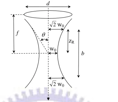
The transverse resolution of OCT imaging is the same as that in the conventional optical microscopy and is determined by the diffraction limited spot size of the focused beam. The minimum spot size limited by diffraction is inversely proportional to the numerical aperture (NA) of the focusing optics. For a Gaussian beam, the transverse resolution or the minimum beam spot size is given by:

NA d f w x ⋅ ≈ ≈ = = Δ π λ π λ πθ λ 4 2 2 2 ₀ ,

where w is the beam waist, ₀ θ is the convergence half-angle, d is the

spot size of the beam on the objective lens and f is the focal length [7]. It means finer transverse resolution can be obtained by using larger NA which corresponds to a smaller spot size. However, the transverse resolution is also related to the depth of field or the confocal parameter b , which is two times the Rayleigh range:

λ π λ π 2 ) ( ) ( 2 2 2 2 0 x w z b = _R = = Δ ,

Fig. 1.4 shows the relationship between the minimum spot size and the depth of field. Thus, similar to conventional microscopy, improving transverse resolution involves a trade-off in decreasing the depth of field at the same time. Typically, focusing optics with low NA is commonly employed in OCT because they have a relatively large Rayleigh range and thus provide longer depth of focus. In this way the axial resolution will be dominated by the coherence length of the light source, which is shorter than confocal parameter.

1.1.3 Other types of OCT

To achieve real-time imaging, imaging speed becomes an important parameter in OCT. Recently, two types of Fourier domain detection have been developed to increase the imaging speed dramatically. These techniques are known as Fourier/spectral domain detection (SD-OCT) [8~11] and swept source/Fourier domain detection (SS-OCT) [12~14]. Unlike TD-OCT, SD-OCT performs high-resolution detection by measuring the interference spectrum with a low-coherence light source and a spectrometer. SS-OCT utilizes an interferometer with a narrow-bandwidth, frequency-swept light source and detectors to measure the interference signal as a function of time. The main reason that Fourier domain detection has a powerful sensitivity advantage over the time domain detection is that it essentially measures all the backscattered light simultaneously [14~16]. On the other hand, only the transverse scanning has to be performed. The depth information is provided by an inverse Fourier transform of the spectrum of the interference between the

θ w0 2w0 f d 2w0 zR b

Fig. 1.4 The relationship between minimum spot size and depth of field.

backscattered light from fixed reference and sample. Such a sensitivity enhancement in Fourier-domain OCT corresponds to a boom in image speed.

For more information and details about OCT, see the reference [17].

1.2 Broadband emitters for OCT

In order to meet the requirement of broad spectrum, superluminescent diodes (SLDs) and femtosecond laser are two kinds of major low-coherence light sources in OCT.

1.2.1 Superluminescent Diodes (SLDs)

Briefly, SLD is the light output from laser structure below threshold. Operating at amplified spontaneous emission (ASE) and suppressing stimulated emission, SLD achieves wider spectrum than laser does by tilting the ridge structure. Compared to its competitive light sources, SLDs are now considered the most attractive light emitters due to their small size, easy use, and much lower price.

In the past, SLD could not become an ideal light source for OCT application because it was unable to meet all the demands simultaneously, including high optical power, broad spectrum, and negligible parasitic spectrum modulation. Early medical OCT application employed commercially available GaAs-based SLD, which operated at near 800nm with bandwidths of ~30 nm to achieve axial resolutions of ~10 μm in tissue. Besides, there have been advances in multiplexed SLD. Bandwidths broader than 150 nm but with limited power, which corresponds to axial resolutions as fine as 3-5 μm, can be achieved [18]. However, for scattering tissues, light sources with longer wavelengths are

essential to get enough penetration depth. At the same time, increasing of spectral wavelength results in increasing of coherence length which is proportional to square of wavelength. Therefore, SLD with centered wavelength at 1300 nm must be at least 2.5 times broader than 800nm counterpart to achieve the same resolution. Although much broader spectrum in multiple quantum well (MQW) and quantum dot (QD) SLDs at 1300~1550 nm have been demonstrated, spectral width of the most powerful (10~20 mW from SM fiber) commercial SLDs at 1300 nm is currently around 60~70 nm [19~20].

1.2.2 Femtosecond Lasers

Femtosecond lasers are the other powerful light sources for applications of ultra-high resolution OCT because they can generate extremely broad bandwidth spectrum at near infrared (IR) region. The Kerr lens modelocked (KLM) Ti:Al2O3 is the most commonly used technique in femtosecond optics and ultra-short pulse application. Through the development of double-chirped mirror technology (DCM) [21], high-performance Ti:Al2O3 laser has been implemented recently. Using state-of-the-art Ti:Al2O3 lasers, axial resolution of ~1 μm can be demonstrated [22]. Fig. 1.5 shows a comparison of the spectrum, autocorrelation function and its demodulated envelope (coherence length) of a typical SLD and a Ti:Al2O3 laser. A pioneering study of UHR-OCT in the retina reported by Drexler et al. shows axial resolution of ~3 μm by using a femtosecond laser light source [23]. In combination with nonlinearity, air-silica microstructure fibers or tapered fibers, Ti:Al2O3 laser can generate broadband continuum and achieve axial resolution of ~1 μm in the different spectral region ranging from visible to near IR [24~26]. Despite of their outstanding performance in bandwidth,

femtosecond lasers are criticized due to its relatively high cost and complex. Recently, new Ti:Al2O3 lasers operate with much lower pump power and therefore greatly reducing cost has been developed [27].

1.3 Overview of Semiconductor Quantum Dot

Lasers

Self-assembled quantum confined nanostructures, in the form of quantum dots, have been paid lots of attention due to its near delta-function of density of states (DOS) [28]. Ultralow threshold current density Jth [29], better temperature stability T0 [30], high modulation bandwidth [31], low chirp [32], and small linewidth enhancement factor have been demonstrated [33]. Limited by the number of quantum dot (QD), the gain in QD saturates rapidly at a certain level, gst, with increasing current density [34], which is the main difference of QD laser behavior from quantum well (QW) system. After the gain saturation at ground state (GS), carriers start accumulating at excited states (ES) and then achieve its threshold condition. For a specific laser device, GS

Fig.1.5 Optical bandwidth, interference signal and point spread function using a typical SLD and a femtosecond Ti:Al2O3 laser. For ultra-high resolution OCT, a broadband femtosecond laser with spectrum bandwidth ~260 nm can achieve a free space axial resolution of 1.5 μm.

and/or ES lasing will be determined by its cavity length, density of QD, driving current, and other structural factors.

Broad-spectrum, high-power and highly efficient semiconductor light sources are strongly desirable for sensing and low-coherence imaging applications such as OCT. With higher power than SLD and more compactness than femtosecond laser, broadband semiconductor laser is more competitive if real supercontinuum broad bandwidth can be performed. Nevertheless, because of active material growth technology and fundamental physics, a conventional QW laser generally produces a narrow spectrum with a spectral width of the subnanometer order for a single-frequency laser to a few nanometers for multi-longitudinal mode lasers. Recently, simultaneous two-state lasing from the GS and ES has been observed from QD lasers with well-separated wavelength emissions [35]. Except for incomplete gain clamping at threshold stated as before, this behavior is also attributed to the retarded carrier relaxation process in QDs, which is also known as the phonon-bottleneck [36]. On the other hand, to achieve real broad laser spectrum of tens of nanometer scale from the QD laser, high dispersion in QD size and small energy spacing between quantized energy states that lead to the broadened optical gain characteristics play important roles as well. In fact, optical line broadening of the emission spectrum of a transition depends on both homogeneous and inhomogeneous broadening mechanisms. Besides the contribution of large dot size fluctuation towards inhomogeneous broadening phenomenon, mechanisms such as acoustic and optical phonon-carrier interaction, lifetime broadening, and carrier-carrier interaction greatly affect the homogeneous linewidth in semiconductors [37]. Lately, NL Nanosemiconductor demonstrated the extended lasing spectral width with uniform intensity distribution (only a 3dB modulation) of about 75 nm [38~39]. A broad lasing spectrum of 40 nm was also

demonstrated by H. S. Djie et al [40].

In this study, specially designed chirped-multilayered QD (CMQD) lasers with three kinds of different wavelength InAs-InGaAs QD stacks were grown. Besides, we have set up a fiber-based, delay-tunable Mach-Zehnder interferometer to measure the interferograms or autocorrelation function which can be used to quantitatively determine the coherence length of a light source. Except for achieving low threshold current density and high saturated modal gain, we demonstrate broad spectrum of 29 nm in this structure and expect that it could be improved to satisfy all the demands for a suitable OCT light source someday.

Chapter 2

Theoretical Fundamentals

2.1 Coherence Theory

In optics, the original sense of the word coherence was attributed to the ability of radiation to produce interference phenomena. Nowadays, the term of coherence is defined more specifically by the correlation properties between quantities of an optical field. Common interference is the simplest phenomenon showing correlations between light waves. It is convenient to divide coherence effects into two classifications, temporal and spatial. The former relates directly to the finite bandwidth of the light source, the latter to its finite extent in space. Experimentally, Michelson introduced a technique for measuring the temporal coherence by Michelson interferometer. Spatial coherence is illustrated by the double-slit experiment of Young. When it comes to coherence length, what we mainly consider here is temporal coherence.

2.1.1 Temporal Coherence

First of all, we consider the path of rays in a Michelson interferometer which is shown in Fig. 2.1. The incident light is divided into two beams by a beam splitter. One beam is reflected back onto itself by a fixed mirror, the other one is also reflected back by a mirror which can be shifted along the beam. Both reflected beams are divided again into two by the beam splitter, whereby one beam from each mirror propagates to a photodetector (PD). The idea of this arrangement is to superimpose a light wave with a time-shifted copy of itself.

Let E be the light wave that reaches the screen via the fixed mirror ₁

and E be the one that reaches the PD via the movable mirror. Then we ₂

have at a point on the PD, when the incoming wave has been split evenly at the beam splitter,

) ( ) ( ₁ 2 t =E t +τ E , or E1(t) =E2(t−τ). (2.1)

The wave E₂ thus has to start earlier to reach the screen at time t due

to the additional path of length d2 . The quantity τ depends on the mirror displacement d according to

c d

2 =

τ . (2.2) On the PD, the interference of both waves given by the superposition of the wave amplitudes:

) ( ) ( ) ( ) ( ) (t =E₁ t +E₂ t = E₁ t +E₁ t+τ E . (2.3)

This superposition is not directly visible. A photodetector with a finite integration time detects the superposed light beams and provides the integrated/averaged intensity: 〉 + + 〈 = 〉 〈 = * 2 1 2 1 * _{( )( )} E E E E EE I 〉 〈 + 〉 〈 + 〉 〈 + 〉 〈 = * 2 1 * 1 2 * 2 2 * 1 1 E E E E E E E E Fixed mirror d E2 E1 E = E1 + E2 Light Movable mirror Beam splitter Interference fringes

} Re{ 2 * ₂ 1 2 1 + + 〈 〉 =I I E E } Re{ 2 2 * ₂ 1 1 + 〈 〉 = I E E . (2.4)

The total intensity on the PD is given by the sum of the intensity I of ₁

the first wave and I of the second wave and an additional term, the ₂

interference term. The meaningful information is contained in the expression 〈 2〉

*

1E

E . With Eq. (2.1) this gives rise to the definition:

〉 + 〈 = Γ( ) *( ) ₁( ) 1 τ τ E t E t

∫

+ − ∞ → + = 2 2 1 * 1 T ( ) ( ) 1 lim m m m T T m dt t E t E T τ . (2.5) ) (τ

Γ is known as the complex self coherence function. It is the autocorrelation function of the complex light wave E₁(t). We then get

)} ( Re{ 2 2 )} ( Re{ 2 ) I(τ =I₁ +I₂ + Γ τ = I₁ + Γτ . (2.6)

The complex self coherence function Γ(τ) can be normalized:

) 0 ( ) ( ) ( Γ Γ = τ τ γ . (2.7)

The magnitude γ(τ) is called the complex degree of self coherence. Because Γ(0)=I₁ is always real and is the largest value that occurs when we take the modulus of the autocorrelation function Γ(τ), we have

1 ) (τ ≤

γ . (2.8)

Then the intensity I(τ) can be written by )} ( Re{ 2 2 ) I(τ = I₁ + I₁ γ τ )}) ( Re{ 1 ( 2 ₁ + γ τ = I . (2.9) Actually, )Γ(τ and γ(τ) are not directly obtainable. It is, however, easy to determine the contrast K between interference fringes. This quantity has been used by Michelson who called it visibility and defined

it via the maximum and minimum intensity I_max and I_min as min max min max I I I I K + − = . (2.10)

Obviously, the maximum and the minimum intensity of the interference fringes do not occur at the same time shift of the light waves; that is, K is a function of τ . Let τ₁ and τ₂, τ₂ > , be the time shifts belonging τ₁ to adjacent interference fringes of I_max(τ₁) and I_min(τ₂). Then the

contrast )K(τ is defined on the interval [τ₁,τ₂) by

) ( ) ( ) ( ) ( ) ( 2 min 1 max 2 min 1 max τ τ τ τ τ I I I I K + − = . (2.11) 1 2 τ

τ − corresponds to half a mean wavelength, which is small compared to the duration of the wave train to be investigated. Only in this case does the definition make sense. According to Eq. (2.6), the maximum intensity is attained at maximum Re{Γ(τ)}, occurring at τ₁, and the minimum intensity at minimum Re{Γ(τ)}, occurring at τ₂. It follows, for τ taken from this interval, that

) ( )} (

Re{Γτ₁ = Γτ and Re{Γ(τ₂)}=−Γ(τ). (2.12)

This leads to the intensities

) ( 2 2 )} ( Re{ 2 2 ) ( _{1 1 1 1} max τ = I + Γ τ = I + Γτ I , (2.13) ) ( 2 2 )} ( Re{ 2 2 ) ( _{2 1 2 1} min τ = I + Γτ = I − Γτ I , (2.14)

and to the contrast function

) ( 2 2 ) ( 2 2 ) ( 2 2 ) ( 2 2 ) ( 1 1 1 1 τ τ τ τ τ Γ − + Γ + Γ + − Γ + = I I I I K ) 0 ( ) ( ) ( 4 ) ( 4 1 1 Γ Γ = Γ = Γ = τ τ τ I I ) (τ γ = . (2.15)

coherence. This is valid for two waves of equal intensity, otherwise some prefactors will arise. Fig.2.2 shows the self coherence function Γ(τ) in the complex plane (up) and contrast function K(τ) (down) for different light sources. Light in the large range in between the two limiting cases, completely coherent and completely incoherent, is called partially coherent. The following cases are distinguished (τ ≠0, γ(0) =1) :

, 0 ) ( , 1 ) ( , 1 ) ( 0 incoherent completely coherent partially coherent completely ≡ ≤ ≡ ≤ τ γ τ γ τ γ

All real light sources are partially coherent. Most part of natural and artificial light sources have a monotonously decreasing contrast function; for instance, the light from a mercury lamp. To characterize the decay of the contrast function, the coherence time τ_c is introduced. It is defined as the time delay when the contrast function has dropped to 21/ or possibly 1 of its maximum value. In other words, it specifies the /e

duration of time that a source maintains its phase. Equivalently to the coherence time, the coherence length

c τ c l_c = , (2.16) 0

τ

) (τ K 0 1 0 0

τ

) (

τ

K 1 0 0 ) (τ K

τ

1 Γ Re Γ Im ) (τ Γ τ Γ Re Γ Im ) (τ Γ 0 ≠ τ τ = 0 Γ Re Γ Im ) (τ Γ

Completely coherent Completely incoherent Partially incoherent

Fig.2.2 Graph of the self coherence function Γ(τ), and the contrast function )K(τ for light from completely coherent, completely incoherent, and partially coherent light, respectively.

is used for characterizing the interference properties of light. Typical values of the coherence length are some micrometers for incandescent light and some kilometers for single-mode laser light.

In a word, to determine the coherence length of some light source experimentally, all we have to do is to measure the interferogram or autocorrelation with enough path difference by a delay-tunable interferometer. After extracting the AC component and then detecting its envelope, we can define the FWHM of this profile as the coherence time. Coherence length will be obtained after multiplying coherence time by the light speed, c .

2.1.2 Wiener-Khinchin Theorem

When it comes to coherence of a light source, its spectral bandwidth plays an important role. A connection between the autocorrelation of a function and its Fourier transform is established by the Wiener-Khinchin theorem. It states that the autocorrelation and the power spectrum of a function are Fourier transforms of one another. In the time domain, if

) (t

f is a radiated electric field, f(t)2 is proportional to the radiant

flux or power, and the total emitted energy is proportional to f t dt

2

0 ( )

∫

∞ . In the frequency domain, F(ω) is the Fourier transform of f(t), which

is called the field spectrum. (_ω)2 *(_ω) (_ω)

F F

F = must be a measure of

the radiated energy per unit frequency interval, which is sometimes called the power spectrum. In other words, F(ω)2 is just what we measure from the optical spectrum analyzer (OSA).

According to the definition, the autocorrelation of f(t) is denoted by dt t f t f

∫

+∞∞ + = Γ₍τ_{) -} *_{( ) (} τ₎ (2.17) 0

Let )F(ω be the Fourier transform of f(t), denoted by FT{ tf( )}.

∫

+∞∞ − = = ( ) _- ( ) )} ( {f t F f t e dt FT ω iωt (2.18)

The autocorrelation can be rewrite to

∫

∫

∫

+∞∞ − ∞ + ∞ ∞ + ∞ + = - - × + * -* _{( ) ] ( )} 2 1 [ ) ( ) (t f t dt F e d f t dt f ω i t ω τ π τ ω (2.19)

Changing the order of integration, we obtain

ω τ ω π ω τ ω π ω d t f FT F d dt e t f F i t ( ) { ( )} 2 1 ] ) ( [ ) ( 2 1 -* -* _{+ = × +}

∫

∫

∫

+∞∞ ∞ + ∞ − ∞ + ∞

In the last integral, notice that

} ) ( { ] ) ( 2 1 ) ( ( ) -ωτ τ ω _{ω ω} ω π τ i t i e F IFT d e F t f + =

∫

+_∞∞ + + = +

IFT means inverse Fourier transform. Then, Eq. (2.19) becomes

ω ω ω π τ ωτ d e F F dt t f t f +_∞∞ +i ∞ + ∞

∫

∫

+ = ( ) ( ) 2 1 ) ( ) ( -* -* (2.20)

and both sides are functions of the parameter τ. If we take the transform of both sides, Eq. (2.20) then becomes

2 ) ( )} ( { τ F ω FT Γ = (2.21)

This is a form of the Wiener-Khinchin theorem. It allows for determination of the spectrum by way of the autocorrelation of the generation function. By the way, Wiener-Khinchin theorem is the main idea in Fourier-Transform Spectroscopy (FTS). The variable part of the interference function, on Fourier transformation, yields the spectrum. It is now used widely in the infrared region because of the improved signal-to-noise (S/N) ratio, high throughput, and high resolution possible with it.

2.2 Semiconductor Quantum Dots

In this chapter, I will discuss about the density of state (DOS) in semiconductor, the formation of quantum dots and the carrier transition between excited states and ground state in quantum dots.

2.2.1 Ideal Quantum Systems

In semiconductor, an interaction between electrons of neighboring atoms is sufficiently strong. This interaction splits an atomic energy level to as many sublevels as the number of atoms contained in the system. These sublevels are grouped in bands. The width of a band is controlled by the strength of interaction of electronic shells, that is, interatomic spacing. In semiconducting crystals, where the interatomic spacing is set by the lattice constant in the range of few angstroms, the width of the order of several electron volts is typical for the valence (the last occupied) and conduction (the first empty) bands. The energy gap, which exists between these two allowed bands, contains no electronic states and is known as the forbidden band. Its width ranges from several electron volts (insulators) to zero (metals).

The number of allowed states within a given band is roughly equal to the number of atoms inside the crystal. It is as many as few ₁₀ 22

electrons per cubic centimeter. However, these states are not distributed uniformly within the band. To characterize this distribution, a DOS is introduced. DOS is a function of energy ρ(E) and it is a measure of allowed electronic states within unit energy interval per unit volume of crystal: ) / )( / 1 ( ) (E = V dN dE ρ . (2.22)

DOS has dimensionality of energy-1 volume-1 and shows how many states are available within unit energy interval around some energy E in a crystal of unit volume. Eq. (2.23)~(2.30) are the corresponding dispersion relation and DOS for four kinds of ideal quantum systems:

Bulk: 0 2 2 2 * 2 ) ( 2 ) , , ( ) ( k k k E m k k k E k E ρ = _{x y z} = η _x + _y + _z + (2.23) 2 1 0 2 2 3 2 * 3 _{( )} 2 ) 2 ( ) (E m E E D = − π ρ η (2.24) Quantum Well (QW): 0 2 2 2 * 2 ] ) ( [ 2 ) , ( ) ( E L n k k m k k E k E z y x y x n = + + + = η π ρ (2.25) ) ( ) ( ₂ * 2 n n z D E E L m E =

∑

Θ − η π ρ (2.26)

Quantum Wire (QWire):

0 2 2 2 * 2 , [ ( ) ( ) ] 2 ) ( ) ( E L n L m k m k E k E z y x x n m = + + + = η π π ρ (2.27)

∑∑

₋ − = n m m n QWire D E E m n E _, 12 * 1 _{( )} 2 _{( )} η π ρ (2.28) Quantum Dot (QD): 0 2 2 2 * 2 , , [( ) ( ) ( ) ] 2 ) ( E L n L m L l m E k E z y x n m l = + + + = η π π π ρ (2.29)

∑∑∑

− = n m l m n l QD D E E n E) 2 ( ) ( _{, ,} 0 _δ ρ (2.30)

where E is the energy of the band edge of the corresponding band; ₀

) (E −E_n

Θ is step-function which returns zero if E <E_n or unity

otherwise; δ(E − E_{n, lm,} ) is the delta-function; and nQwire (cm

-1_{) and} QD

(cm-2) are the surface density of quantum wires and QDs, respectively. Fig. 2.3 illustrates the schematic view and DOS of various ideal quantum nanostructures.

2.2.2 Structural Characteristics of Quantum Dots

To realize quantum dot structure, various techniques based on self-organization have been intensively investigated recently instead of conventional lithography-based or regrowth technology. The self-organized quantum dots have high crystal quality, and they are small enough to exhibit quantum confined effects. Among several techniques, the Stranski-Krastanow (S-K) growth in highly strained heteroepitaxial systems is most studied by using molecular beam epitaxy (MBE) or metalorganic chemical vapor deposition (MOCVD). Cluster formation occurred during epitaxial growth of a semiconductor material on top of another one that has a lattice constant several percent smaller, for instance, InAs on GaAs substrate. For the first few atomic layers, the atoms arrange themselves in a planar layer called the wetting layer. As the

3D : Bulk 2D : QW 1D : QWire 0D : QD

epitaxial overgrowth proceeds, the atoms tend to bunch up and form clusters (quantum dots). It is energetic favorable, because the lattice can elastically relax the compressive strain and thus reduce strain energy within the islands.

The size of the islands can be adjusted within a certain range by changing the amount of deposited dot material. The change in size corresponds to an energy shift of the emitted light, which is due to the altered carrier confinement and strain in the dots. On the other hand, to obtain the information about structural and morphological characteristics of QDs, atomic force microscopy (AFM), scanning tunneling microscopy (STM), transmission electron microscopy (TEM), and photoluminescence (PL) spectroscopy are the most well-known and widely adopted methods. In fact, except for its shape and size, the energetic property of QDs also depends on the thickness and the highness of potential barrier of the capping layer.

2.2.3 Carrier transition in Quantum Dots

To achieve population inversion, fast intraband relaxation time is required. In quantum well systems, the typical intraband relaxation lifetime is about 0.1~1 picoseconds (ps). However, due to the lack of phonons needed to satisfy the energy conservation rule, the carrier relaxation into the discrete ground state is significantly slowed down in QDs (the so-called phonon bottleneck). Retarded carrier relaxation, with a lifetime ranging from several tens to hundreds of picoseconds, has been observed in many experiments using time-resolved PL. Even though Auger-like process and carrier-carrier scattering have been suggested for possible fast relaxation channels with a lifetime of 10 ps or less, the bottleneck effect still affects QD laser performance to some extent, such

as the degradation of threshold current and the external quantum efficiency.

2.3 Quantum Dot Lasers

Laser is an acronym meaning “light amplification by stimulated emission of radiation”. A semiconductor, owing to a possibility of direct injection of electrons to the active region, gives an opportunity to make compact and efficient laser device. Basically, laser consists of the light-amplifying region where inverse population takes place and the positive optical feedback.

2.3.1 Basic Principles of Diode Lasers

In semiconductor, photon emission due to electron return from the conduction band to the valence band can be considered as radiative recombination of electron-hole pair. However, electron can also lose its energy non-radiatively. For any light-emitting device, too non-radiative recombination results in additional consumption of excited electrons and has to be minimized. Actually, there are two possible mechanisms when photon emission occurs. One is spontaneous emission with arbitrary phase, arbitrary direction and at an unpredictable instant of time. Otherwise, photon emission can be triggered by another photon, the so-called stimulated emission, and holds all the properties of the initial one.

Under condition of thermal equilibrium, light emission is balanced by the light absorption. The following equation connects the electron, n , and hole, p , concentrations:

2

i n

np= (2.32)

Here n is intrinsic concentration governed by temperature. To _i

overcome this loss of photons, larger population of the upper level than that of the ground level is required. This situation, the so-called population inversion, is obviously non-equilibrium and can be reached by some external influence, such as illumination or current injection.

2

i n

np> (2.33)

To describe concentrations of electron and hole, their non-equilibrium Fermi levels, F and _C F are introduced. A condition of inverse _V

population means that electron population probability of the conduction band state f_C(E_C) having energy E is higher than that of the valence _C

band state with E energy: _V

) ( ) ( _{C V V} C E f E f > (2.34)

where population probability of carriers in semiconductor follows Fermi-Dirac distribution: ) / ) exp(( 1 1 ) ( T k F E E f B C C C C = _{+ −} (2.35)

Taking into account these expressions, the condition of inverse population comes to the following inequality:

g V C V C F E E E F − > − = (2.36)

It means that energy separation of electron and hole Fermi levels has to be larger than the band gap of a semiconductor, E . At this moment, so-called transparency takes place. Material becomes transparent for light of the given energy ηω =E_C −E_V . The corresponding density of

injection current is known as the transparency current density.

2.3.2 Optical Gain and Laser Threshold

When light propagates through a medium, its intensity, Φ , will be attenuated due to light absorption, which is characterized by absorption coefficient α. Mechanisms which contribute to optical loss have various origins. They usually are divided into the output (mirror) loss, α_m, caused by light output from the cavity and the internal loss, α_i, which combines the effect of all the other mechanisms. However, if population inversion takes place in the medium, the absorption coefficient changes sign to negative due to stimulated emission dominates the light absorption. To emphasize these two different cases of light absorption or light amplification, optical gain coefficient, G , is introduced. Now we consider the output loss inside a Fabry-Perrot cavity as shown in Fig. 2.4.

Let us assume that light propagating from the left to the right facet has intensity Φ at its initial position at the left facet. Over the length L ₀ it becomes to Φ₀exp[(G−α_i)L]. After partial reflection at right facet having reflectivity R , a beam of intensity ₁ R₁Φ₀exp[(G −α_i)L] starts

from right to left. In the similar manner, the intensity of the light becomes equal to R₁R₂Φ₀exp[2(G−α_i)L] at its initial position after a round trip, where R is the left-facet reflectivity. In steady state (at threshold), this ₂

Fig. 2.4 Light propagation and its intensity in a round-trip cycle inside the Fabry-Perrot cavity.

2 R R₁ L 0 Φ Φ₀exp[(G−α_i)L] ] ) exp[( 0 1 G L RΦ −α_i ] ) ( 2 exp[ 0 1 G L RΦ −α_i ] ) ( 2 exp[ 0 2 1R G L R Φ −α_i

round trip results in no change of the light intensity. ] ) ( 2 exp[ 0 2 1 0 =RR Φ Gth −αi L Φ (2.37) m i i th R R L G =α + ln( 1 )=α +α 2 1 2 1 (2.38) th

G is the threshold gain. At this moment, the injected current density is

called the threshold current density J_th. The optical confinement factor

Γ should be introduced when we consider the interaction between charge carriers and the light. It is defined as the ratio of the integrated light intensity with the region of inversion population to the total optical intensity throughout the laser structure. Different transverse optical modes will have different overlap with the active region. Therefore, the optical gain in Eq. (2.38) corresponds to a certain mode and is known as the modal gain as opposed to the material gain. Specifically, the modal gain is a product of the Γ - factor of the given q mode and the material _th

gain, g_mat: mat q q g G =Γ (2.39)

2.3.3 Characteristics of Quantum Dot Lasers

For an individual self-organized QD, its electronic structure is very similar to the ideal case. There is a set of atomic-like quantum levels composed of several excited states and ground state. However, in contrast to the ideal array of identical QDs, self-organized islands differ greatly from each other in their size , shape, and other parameters affecting the energy of the quantum level. Namely, the quantum energy of real QD arrays is statistically determined rather than the zero-dimensional DOS of the individual QD. The DOS is maximum at the energy that corresponds

to the most probable QD size. In fact, the DOS of the array is characterized by a set of subbands that originates from inhomogeneously broadened quantum level of the GS and ES of individual QDs. Typically, the energy separation between ground state (GS) and excited state (ES) in QD is about 40~70 meV.

Compared to QW laser, the saturated gain, G , of QD laser is _sat

much lower and proportional to the DOS at the maximum:

Δ ⋅ ∝ ∝ max / QD i QD sat g n G ρ (2.40)

where g is the level degeneracy ( g =1 for the GS and ES is usually _i

characterized by g_i >1), n_QD is surface density of QD and Δ is the

energy width of the DOS. Real QD array will decrease G_sat due to

inhomogeneous broadening. On the other hand, the saturated gain can be increased by means of several QD planes or denser QD arrays in each plane. However, the transparency current density which is also proportional to the total surface density of the QD array will be traded off. In a word, the competition between the transparency current density and the gain saturation determines the threshold current density at the given cavity loss.

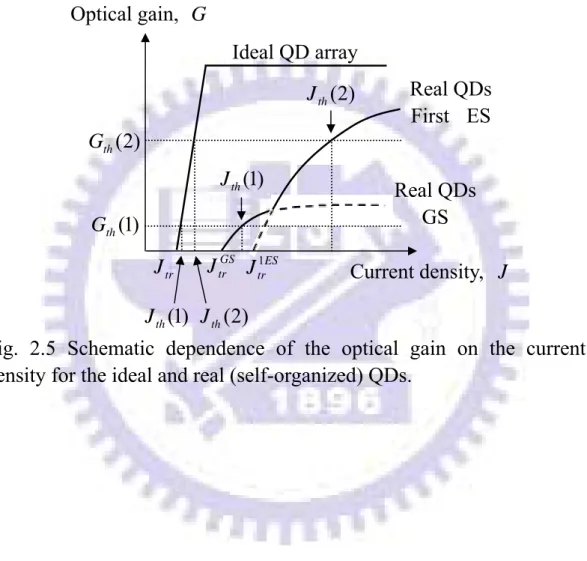
In addition to the GS level, it was observed that one or more ES levels can be thermally populated to give an additional contribution to the threshold current density [41]. With higher degeneracy, these ES levels have higher saturated gain. Thus, the transition of the lasing emissions from the GS to the ES can be observed with increasing total loss. The situation is illustrated in Fig. 2.5, where the gain-current dependence is schematically shown for ideal as well as self-organized QD arrays. By the way, it has been shown that the experimental dependence of the optical modal gain on the threshold current density can be well fitted by the following empirical equation [42]:

)] exp( 1 [ tr tr sat J J J G G= − −γ − (2.41)

where G_sat and J_tr are usual meaning of saturated gain and

transparency current density, γ is an additional dimensionless gain parameter which can be treated as a non-ideality factor.

Fig. 2.5 Schematic dependence of the optical gain on the current density for the ideal and real (self-organized) QDs.

Current density, J Optical gain, G Ideal QD array Real QDs First ES Real QDs GS ) 2 ( th G ) 1 ( th G tr J J_trGS ES tr J1 ) 1 ( th J ) 2 ( th J ) 1 ( th J J_th(2)

Chapter 3

Experimental Techniques

3.1 Coherence Length Measurement

Compared with measuring the spectrum of some light sources, the measurement of coherence length provides a more direct way to judge whether an emitter is suitable or not for OCT application. To achieve the goal, we have set up a fiber-based, delay-tunable Mach-Zehnder interferometer.

3.1.1 Experimental Setup

The automatic, delay-tunable interferometer is re-equipped from the commercial, manually path-tunable MZI-VAR 1300, which is used as the frequency clock in SS-OCT originally and is produced by Thorlabs. Fig. 3.1 shows the scheme of the whole system. Roughly speaking, the system is composed of three components, fiber-based Mach-Zehnder interferometer (MZI), computer-controlled translation stage and signal digitizer. They function as doing interference, providing path difference

Fig.3.1 The scheme of the coherence length measurement system.

Light Source Detector

Fiber Coupler Fiber Coupler Translation Stage Polarization Controller GRIN Lens Collimator Built-in Digitizer Computer

and demonstrating signal processing, respectively. Compared to free-space Michelson interferometer, the advantage of the fiber-based MZI is that it doesn’t require aligning the light beams except for the face-to-face collimators.

In short, the MZI is constructed by two 50/50 couplers. A translation stage driven by a computer-controlled actuator is used to change the optical delay in one arm of the MZI. Fig. 3.2 shows the photo of the MZI. The polarization controller in the other arm of MZI can be used to optimize the polarization status in the fiber and maximize the interference fringe contrast in the detector output. One of the two output ports of the second 50/50 coupler is connected to a photodetector (PD). Then the interference signal from the PD will be sampled by a high-speed digitizer and the data can be saved.

The actuator, Z825, with a maximum traveling range of 25mm and a minimum resolution of 29 nm, is produced by Thorlabs. In other words, only light sources with coherence length shorter than 25 mm can be defined by this system. The high-speed digitizer, NI 5122, with a maximum sampling rate of 100M points per second, is a product of National Instrument. Narrow-shape interferogram can be obtained by means of setting appropriate traveling velocity and enough sampling rate.

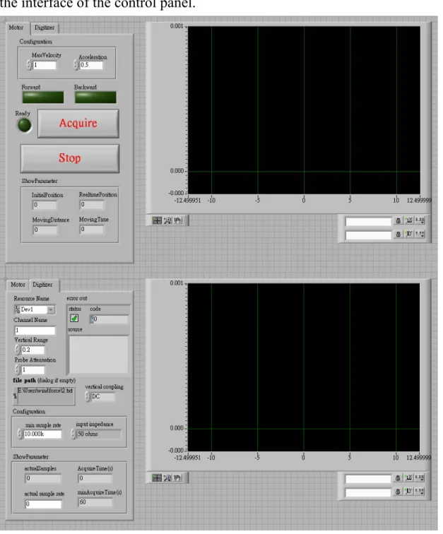
Labview software is used to controlled the actuator and digitizer simultaneously and output the digital interferogram data. Fig. 3.3 shows the interface of the control panel.

Followings are some crucial issues that have to be concerned in this system. First, to define the coherence length correctly, the traveling range of the actuator must pass through the point of zero path difference. It can be proved by the characteristic of perfect symmetry of the

interferogram. Second, the face-to-face collimators must be aligned as good as possible to achieve nearly equal receiving power during translation. Finally, due to the sensitivity of interference, the whole system including all the fibers must remain stationary during the measurement. Any fluctuation will change the polarization state of the fiber output and further make an impact on the interferogram.

3.1.2 The Accuracy of Measurement

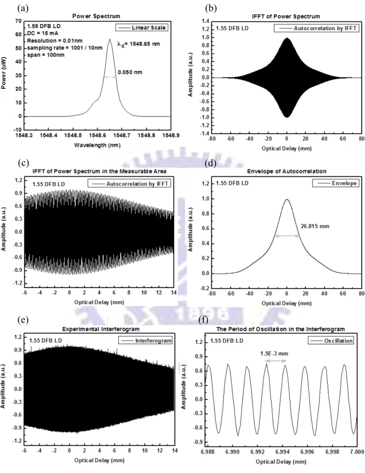
The Wiener-Khinchin theorem provides us a method to verify whether our measurement is accuracy enough or not. The interferogram and the power spectrum form a Fourier Transform pair. We measure the power spectra and interferograms of three commercial lasers. They are 1310 nm MQW-FP LD (multiple quantum well - Fabry-Perot laser diode), 1310 nm MQW-DFB (distributed feedback) LD and 1550 nm MQW-DFB LD and then will be abbreviated by LD#1, LD#2 and LD#3, respectively. The measurement of optical spectrum will be discussed later.

In this regard, an issue must be concerned before performing Inverse Discrete Fourier Transform (IDFT) on linear-scaled power spectrum we measured. According to sampling theorem, an analog signal that has been sampled can be perfectly reconstructed without aliasing from the samples only if the sampling rate exceeds two times of the highest frequency in the original signal. On the other hand, the sampling interval in the time domain is the reciprocal of the sampling range in the frequency domain; the sampling range in the time domain determines the reciprocal of the sampling interval in the frequency domain, and vice versa. In conclusion, to make sure the reconstructed data is without aliasing and is correct, some conditions when measuring the power spectrum must be considered,

such as enough sampling rate and sampling range. By the way, a more efficient algorithm, IFFT (Inverse Fast Fourier Transform), is used to compute the IDFT. More details about these concepts can be referred to textbooks of digital signal processing (DSP) [43].

Fig. 3.4~3.6 show the comparison of (a) the power spectrum in linear scale, (b) IFFT of power spectrum, (c) IFFT of power spectrum in the measurable area (d) envelope detection on IFFT of power spectrum, (e) the experimental interferogram and (f) its detail for the three different light sources. The FWHM of the main peak in the three power spectra (Fig. 3.4~3.6 (a)) are 0.022 nm, 0.012 nm and 0.050 nm, corresponding to theoretical coherence length (Fig. 3.4~3.6 (d)) as long as 64.30 mm, 124.69 mm and 26.82 mm, respectively. As expected, the narrower a spectrum of some light source is, the longer its coherence length will be. Obviously, due to the limitation of our optical spectrum analyzer (OSA), the power spectrum of LD#2 (Fig. 3.5 (a)) may not accurate enough and should be narrower in reality. In other words, its coherence length should be longer than the value above. Besides, the periodic behavior of the carrier wave in the interferogram will be the other evidence to confirm if what we measured is reasonable. The oscillation period of an interferogram directly depends on the central wavelength of a light source. It also can be observed from Fig. 3.4~3.6 (f). Though these coherence lengths longer than 25mm can not be defined experimentally with our interferometer, the accuracy of the measurement can be confirmed by the similarity between theory (Fig. 3.4~3.6 (c)) and our experiment (Fig. 3.4~3.6 (e)).

The interferograms we measured here are all obtained when these lasers are under continuous-wave (cw) mode operation. For most broadband lasers, including our CMQD LDs, relatively high current injection is necessary. However, severe thermal effect induced by highly

35

cw pumping will cause great damage to our devices which are unpackaged and without facet coating. Some differences between interferograms measured at cw and pulsed mode will be discussed later.

Fig. 3.4 (a)The power spectrum in linear scale, (b)IFFT of power spectrum, (c) IFFT of power spectrum in the measurable area (d)envelope detection on IFFT of power

(a) (b) (c) (d) (e) (f) nm 022 . 0 = Δλ

Fig. 3.5 (a)The power spectrum in linear scale, (b)IFFT of power spectrum, (c) IFFT of power spectrum in the measurable area (d)envelope detection on IFFT of power spectrum, (e)the experimental interferogram and (f)its detail for LD#2.

(a) (b)

(c) (d)

Fig. 3.6 (a)The power spectrum in linear scale, (b)IFFT of power spectrum, (c) IFFT of power spectrum in the measurable area (d)envelope detection on IFFT of power spectrum, (e)the experimental interferogram and (f)its detail for LD#3.

(a) (b)

(c) (d)

3.2 Characteristics of Laser Diode

3.2.1 Light - Current - Voltage (L-I-V) Characteristic

L-I-V characteristic is the most fundamental characteristic of a LD. The threshold current (I ), slope efficiency (_th η), turn-on voltage (V ) and ₀

series resistance (R ) of a LD can be immediately determined from a _s

measured L-I-V curve. More parameters, such as internal loss (α_i), model gain ( G ),...etc, can be obtained by analyzing these basic parameters from devices of different cavity length. Fig. 3.7 shows the schematic diagram for the measurement of L-I-V characteristics.

In our L-I-V measurement, laser device is put on a copper stage which is equiped with a TE-cooler to stabilize the temperature of our device. Keithley 2520 pulsed laser diode test system is used for current injection and photocurrent detection. The light output is detected by a Ge detector and eventually will be calibrated mathematically by a well calibrated power meter. In the meanwhile, electrical information will be feedbacked to Keithley when current injection begins. With GPIB-interfaced connection, the whole measurement can be controlled by the computer.

Fig. 3.7 The schematic diagram for the measurement of L-I-V characteristic. Computer LDT-5910 Temperature Controller TE-Cooler KEITHLEY 2520 CW / Pulsed Laser Diode Test System

Probe Station Laser Device GPIB

Detector I