國立高雄大學國際商業管理碩士學位學程
碩士論文
台灣捷運系統對房價的影響
The Impact of Taiwan MRT System on Housing
Prices
研究生:石睿凡撰
指導教授:耿紹勛
致謝詞
就讀研究所的這段期間,有這許多人的幫忙,才能如此順利地撰寫論文並完成 學業。其中最感謝耿紹勛老師耐心地指導我這位外語系畢業的學生,在如期完成碩 士論文的同時,讓我學習了完全不同於大學所學的研究方法及思維。同時也相當感 謝余歆儀老師及陳立文老師在百忙之中,撥空當任我的口試委員,使我能夠順利完 成口試。 感謝曾經教導過我的老師,讓我能在商業管理的這個領域汲取更多知識。也感 謝所上的同學對我的照顧及扶持,我才能如此融入及適應研究所的生活。最後感謝 家人一路的支持及鼓勵,讓我求學過程十分順遂,無後顧之憂地完成碩士學位。i
Content
ABSTRACT ... ii
I. Introduction ... 1
II. Literature Review ... 2
III. Data ... 5
IV. Models ... 10
V. Empirical Analysis and Results ... 12
VI. Conclusions ... 20
ii
The Impact of Taiwan MRT System on Housing Prices
Advisor(s): Dr. Shao-Hsun Keng Department of Applied Economics
National University of Kaohsiung
Student: Jui-Fan Shih IMBA
National University of Kaohsiung
ABSTRACT
MRT system has become the most important transportation for people living in Taipei and Kaohsiung. Many studies have shown that when the distance to public transportation increases, the housing prices decline. While earlier studies examine the effect of the distance to MRT station on housing prices focusing only on one city or one transportation line, this study estimates the effect of the distance to MRT station on housing prices by including the entire MRT lines in Taipei and Kaohsiung. Moreover, we compare the difference in the effect between these two cities.
The results indicate that when the distance to MRT station increases by 1 km, the housing prices decrease by $NT158,432 per ping. When the sample expands to include houses within 3km of the MRT stations, the housing prices decrease by $NT119,468 if the distance to MRT station increases by 1 km. We also show that the relationship between the housing prices and distance to MRT stations is a U shape. The results also show that the distance to the MRT system in Taipei has a greater impact on housing prices than that in Kaohsiung.
1 I. Introduction
As cities grow, public transportation becomes a key factor that affects the urban
development significantly. With a growing number of people move to big cities, traffic
congestion has emerged to be a key issue facing many cities. The Mass Rapid Transit
(MRT) is the main strategy undertaken by many cities to mitigate the problem of traffic
congestion. MRT is an important transportation system developed over the past 20 years
in Taiwan, especially for people who live in the metropolitan areas. With the MRT, people
are able to live in suburban areas without losing the convenience of the big cities.
Consequently, MRT system can not only relieve the pressure of overcrowding in cities
but also expand the boundary of the cities.
In this study, we examine the impact of the distance to MRT station on housing prices
in Taiwan. The research is important because MRT system has become a necessity for
city dwellers and consequently affects the housing price substantially. However, previous
studies focused on the effect of the distance to MRT stations on housing prices either on
a single city or on a single transportation line. Consequently, in this study, we not only
estimate the effect of the distance to MRT stations on housing prices by including all MRT
2 II. Literature Review
The MRT system provides convenient transportation for traveling in the city. Due to
traffic congestion and the difficulty of finding a parking space in urban areas, the distance
to the MRT station has become a key determinant of property values in the city. Bajic
(1983) identified the impact of a subway line in Toronto on the housing prices. The result
showed that the direct savings in commuting from taking the subway should have been
reflected in the housing values. The average amount of savings is estimated to be around
$ US 2,273.
Coffam and Gregson (1998) estimated the impact of the railway on land prices in Knox
County, Illinois. The empirical results suggest that the value of lands increases when the
lands are closer to railroads. The value of lands closer to the railroads is 9% higher than
those that are not. Bowes and Ihlanfeldt (2001) found that proximity to the railroad station,
business activities and crime rates in the neighborhood, affect property values
significantly.
McMillan and McDonald (2004) examined the impact of the completion of rapid transit
line from downtown Chicago to Midway Airport on the prices of single-family houses.
The results show that housing prices are affected by the proximity to subway stations.
3
compared with the real estate far away from transit station between 1986 and 1999.
Armstrong and Rodriguez (2006) suggested that housing prices are 9.6% to 10.1%
higher when residential properties are located within 0.5 miles of the station in Eastern
Massachusetts. In addition, the property values decrease 1.6% for every additional minute
of driving to the railroad station. Dewee (1976) showed that housing prices in Toronto
decrease when the distance to the subway stations increases and distance is one-third of
a mile from the stations.
Debrezion et al. (2007) found that the effects of railway stations on the values of the
commercial property are limited to short distances from the stations. In their study, there
are two different effects to estimate the railway station proximity. The first one is local
station effect, which measures the effect of distance within 0.25 mile from the station.
The second one is the global station effect that measures the effect of coming 250 meters
to the stations.
The empirical results showed that within 0.25 mile from the station, the residential
property value is 12.2% less expensive than commercial property. However, they also
found that at longer distances the effect on residential property values dominates. The
estimates suggested that the value of the residential property is 2.3% higher than that of
4
Damm et al. (1980) used data from Washington Metro and found that property values
are negatively related to the distance to the station. When the distance to a station
increases by 0.1 miles, the rent of an apartment will fall by 2.5% in Washington D.C.
(Benjamin and Sirmans, 1996). Kilpatrick et al. (2007) examine the impact of transit
corridor on the housing prices and the result reveals that proximity to the transit corridor
alone without direct access has negative impact on nearby housing prices
Chernobai et al. (2011) used Spline Regression to estimate the effect of highway on
housing prices in Los Angeles. They found that housing prices show a convex relationship
to the distance to highway. Waddell et al. (1993) also showed that the relationship between
housing prices and the distance of the station is U shape. They used a nonlinear model to
estimate the effect of the distance to the station on land value. The locations of MRT
stations have a different impact on land value. For instance, in downtown Chicago, the
17% increase in the values of residential lands within 1.5 miles from the station can be
attributed to the transit. (McDonald and Osuji, 1995).
In Taiwan, previous studies have shown that MRT system has a significant effect on
housing prices. Penget al. (2009) examined the effect of the completion of Taipei MRT
Red Line on housing prices. The results revealed that the values of houses adjacent to
5
Hong and Lin (1999) estimated the impact of Taipei MRT system and the road width
on housing prices in Taipei. They found that the road width does have a positive effect on
housing prices. Moreover, housing prices increase significantly in the area close to the
MRT stations. More importantly, the relationship between housing prices and the distance
to MRT station is convex.
Tai (2011) also use Taipei MRT System to show that the price effect of MRT station is
nonlinear. Meanwhile, the impact of MRT station is not the same in each distance interval.
Also, there are differences between urban and suburb area. The result showed that the
distance to MRT is station is within 300 meters, the impact on housing prices is more
statistically significant. Moreover, the results also showed that the closer the property lies
within the suburb area, the greater the effect to the housing prices is.
Feng et al. (1994) indicated that the distance to MRT station has a greater effect on
housing prices in downtown. Housing prices in the central business district usually
increase more than the housing price in the outskirt of the central business district and
suburban area. In addition, the increase in the value of land for commercial and office
purpose is greater than that for residential use.
III. Data
6
Kaohsiung collected by Ministry of Interior (Taiwan) from September 2012 to October
2017. The data includes housing prices, the age of the house, size of the house, time
variable and the property type.
All prices are adjusted by CPI and the base year is 2017. In this study, we assume that
the farthest walking distance to the station that can impact housing prices is 3 km. When
the distance exceeds 3 km, the effect of MRT system on housing prices should be small.
To check for robustness, we also examine the impact of walk distance to MRT station on
housing prices with 1.5 km. Because we have the address of the house, we can find the
shortest distance of the property to the MRT station by using Google map.
In addition, we set five-year dummy variables to estimate the time variables from 2012
to 2017 (the base year is 2017). When the transaction year was 2012, YR2012 equals to
one and zero otherwise. Other time dummies are defined similarly. We also set a dummy
variable for Taipei and Kaohsiung. When the observation is from Taipei, then Taipei=1
and 0 otherwise.
There are eight property types listed in the data which are building higher than 11 floors,
building lower than 10 floors, condominium, single-family house, studio apartment,
storefront, commercial and office building and others. We create seven dummy variables
7
In addition, there are missing values for the age of the house. We create a missing
dummy whose value equals 1 if the age of the house is missing and 0 otherwise. At the
same time, we set the age of the house to 0 for observations with missing values. The
final sample of our analyses is 2244.
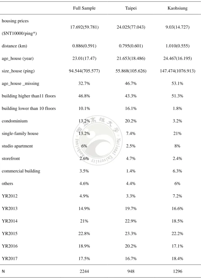
Table 1 is the descriptive statistics of the sample. The average housing prices are
$NT176,920/ping (1 ping = 3.306 square meters); the mean distance to MRT station is
around 0.886 km; the average age of the house is around 23.01 years; twenty-three percent
of our sample has a missing value in the age of the house. The average size of the house
is around 94.544 pings.
If we look at the property types, building higher than 11 floors accounts for 47% of the
sample; condominium and single-family house both account for 13.2 percent; building
lower than 10 floors accounts for 10.1 percent; studio apartment occupies 0.6 percent;
others occupies 4.6 percent; commercial and office building is at 3.5 percent and storefront
is at 2.6 percent.
When we divide the sample into Taipei and Kaohsiung, the estimates show that Taipei
has higher housing prices ($NT240,250/ping > $NT90,300/ping). The average distance
8
Table 1. Definitions, Sample means and Standard deviations of Variables
Full Sample Taipei Kaohsiung
housing prices ($NT10000/ping*) 17.692(59.781) 24.025(77.043) 9.03(14.727) distance (km) 0.886(0.591) 0.795(0.601) 1.010(0.555) age_house (year) 23.01(17.47) 21.653(18.486) 24.467(16.195) size_house (ping) 94.544(705.577) 55.868(105.626) 147.474(1076.913) age_house _missing 32.7% 46.7% 53.1%
building higher than11 floors 46.8% 43.3% 51.3%
building lower than 10 floors 10.1% 16.1% 1.8%
condominium 13.2% 20.2% 3.2% single-family house 13.2% 7.4% 21% studio apartment 6% 2.5% 8% storefront 2.6% 4.7% 2.4% commercial building 3.5% 1.4% 6.3% others 4.6% 4.4% 6% YR2012 4.9% 3.3% 7.2% YR2013 14.9% 19.7% 16.6% YR2014 21% 22.9% 18.5% YR2015 22.8% 23.3% 22.2% YR2016 18.9% 20.2% 17.1% YR2017 17.5% 16.7% 18.4% N 2244 948 1296
9
1.009 km in Kaohsiung. The reason is that the MRT system in Taipei is more extensive
as well as having more lines and stations, compare with Kaohsiung. Thus, the distance to
MRT station in Taipei is shorter.
Houses in Taipei are newer than those in Kaohsiung. The average age of the house is
21.65 years, compared with 24.46 years in Kaohsiung. On the other hand, the size of the
house in Taipei is smaller as well (55.868 pings< 147.474 pings).
The size of the houses in Kaohsiung is bigger than Taipei because the sample of
Kaohsiung contains many transactions of factories and the size of most factories are more
than 200 pings; therefore, the average size of the house is inflated in Kaohsiung
The percentage of building higher than 11 floors is 43% and 51% in Taipei and
Kaohsiung respectively. Building lower than 10 floors with elevator accounts for 16.1%
of the observations in Taipei and 1.8% of the observations in Kaohsiung. Condominium
in Taipei accounts for a higher percentage (20.2%) than in Kaohsiung (3.2%). The
percentage of a single-family house in Taipei is 7.4%, which is lower than the 21% in
Kaohsiung.
Studio apartment accounts for 4.5% and 8% of the sample in Taipei and Kaohsiung
respectively. The percentage of storefront properties in Taipei is 2.7% which is slightly
10
6.2% in Kaohsiung. Others have 4.4% in Taipei and 0.6% in Kaohsiung.
There are 948 observations from Taipei and 1296 from Kaohsiung. The reason why the
number of observation from Taipei is lower than that from Kaohsiung is that house
owners in Taipei don’t want to reveal actual selling prices to the government even though
they will be subject to a fine ranging from $NT30,000 to $NT150,000 per year for failing
to reveal actual selling prices.
IV. Models
We use multiple regression analysis to examine the relationship between housing prices
and the distance to MRT station in Greater Taipei and Kaohsiung. The basic multiple
regression models take the following form:
Price = β0 + β1distance + β2distance2+ β3distance × Taipei + β4distance2×
Taipei + β5age_house + β6age_house_missing + β7size_house + 𝛽𝛽8 Taipei +
𝛽𝛽9bht11 + 𝛽𝛽10blt10 + 𝛽𝛽11condo + 𝛽𝛽12studio + 𝛽𝛽13store + 𝛽𝛽14commercial +
𝛽𝛽15others + 𝛽𝛽16𝑌𝑌𝑌𝑌2012+ 𝛽𝛽17𝑌𝑌𝑌𝑌2013+ 𝛽𝛽18𝑌𝑌𝑌𝑌2014+ 𝛽𝛽19𝑌𝑌𝑌𝑌2015+ 𝛽𝛽20𝑌𝑌𝑌𝑌2016+ 𝜀𝜀
---(1)
Price is housing price per ping adjusted for CPI and the base year is 2017. One ping is
equal to 3.306 square meters. Distance is the distance to station measured in kilometers
11
inverse U shape. Taipei is a dummy variable that equals 1 if the observation is from Taipei
area and 0 otherwise. In addition, distance × Taipei indicates the different effects of
distance on housing prices between Taipei and Kaohsiung. Distance2× Taipei helps
us to know the different decreasing rate of housing prices between Taipei and Kaohsiung.
Age_house is the age of the house which is measured in years. Because there are 33%
of the observations with the age of the house are missing. We use a dummy variable to
cope with the missing values. When the age of the house is missing, then it equals to one
and 0 otherwise. In addition, we set the age of the house to 0 for observations with missing
age. The size_ house is the size of the property and the unit is ping.
Bht11 means the building is higher than 11 floors with elevator. Blt10 means the
building is 10 or lower than 10 floors with elevator. Condo means condominium. Studio
means studio apartment. Store means storefront. Commercial means commercial building.
Others mean other property types such as factory or warehouse. These variables are
dummy variables we create and we set single-family house as the base group. 𝑌𝑌𝑌𝑌2012 to
𝑌𝑌𝑌𝑌2016 are five year dummy variables and the base year is 2017.
According to the regression models above, we can examine the impact of distance on
12 V. Empirical Analysis and Results
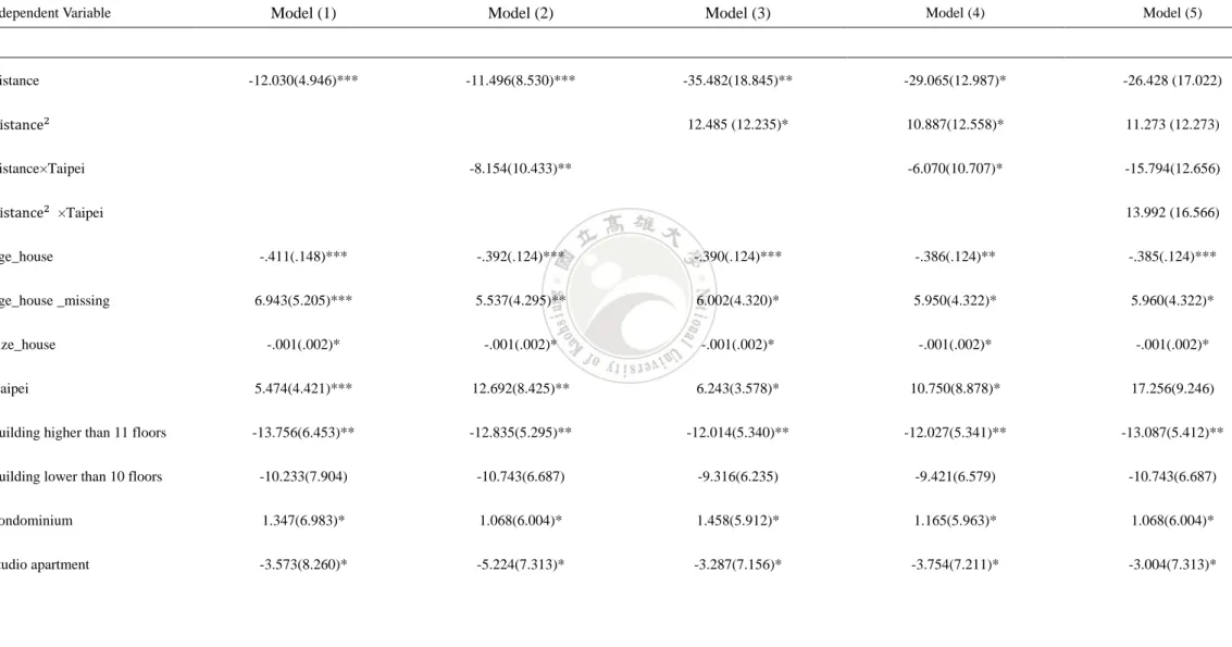
The empirical findings are reported in Tables 2 and 3. Table 2 shows the effect of the
distance to MRT station on housing prices within 1.5 km. Model (1) indicates that distance
to MRT stations, the age of the house, size of the house and Taipei are statistically
significant. More importantly, distance has a negative effect on housing prices. The
estimates show that when the distance to MRT station increases by 1 km, the housing
prices decrease by $NT120,300 per ping.
Model (2) demonstrates that when the distance to MRT station decreases by 1 km, the
housing prices in Taipei is $NT81,540 per ping higher than Kaohsiung. It means that the
MRT system in Taipei has a greater impact on housing prices, compare with Kaohsiung.
Model (3) shows the relationship of the distance to MRT stations on housing prices
between Taipei and Kaohsiung. According to the coefficient of distance2, we can
conclude that the relationship between the housing prices and distance is a U shape.
Model (4) is our main model. The estimates indicate that when the distance increases
by 1 km, the housing prices decrease by $NT158,432 per ping in Taipei, and decrease by
$NT97,732 per ping in Kaohsiung. The relationship between housing prices and distance
13
Table 2. The Effect of Distance on Housing Prices: Distance to MRT station ≦ 1.5 km)
Independent Variable Model (1) Model (2) Model (3) Model (4) Model (5)
distance -12.030(4.946)*** -11.496(8.530)*** -35.482(18.845)** -29.065(12.987)* -26.428 (17.022) distance2 12.485 (12.235)* 10.887(12.558)* 11.273 (12.273) distance×Taipei -8.154(10.433)** -6.070(10.707)* -15.794(12.656) distance2 ×Taipei 13.992 (16.566) age_house -.411(.148)*** -.392(.124)*** -.390(.124)*** -.386(.124)** -.385(.124)*** age_house _missing 6.943(5.205)*** 5.537(4.295)** 6.002(4.320)* 5.950(4.322)* 5.960(4.322)* size_house -.001(.002)* -.001(.002)* -.001(.002)* -.001(.002)* -.001(.002)* Taipei 5.474(4.421)*** 12.692(8.425)** 6.243(3.578)* 10.750(8.878)* 17.256(9.246)
building higher than 11 floors -13.756(6.453)** -12.835(5.295)** -12.014(5.340)** -12.027(5.341)** -13.087(5.412)**
building lower than 10 floors -10.233(7.904) -10.743(6.687) -9.316(6.235) -9.421(6.579) -10.743(6.687)
condominium 1.347(6.983)* 1.068(6.004)* 1.458(5.912)* 1.165(5.963)* 1.068(6.004)*
14
Notes: 2017 = 0, Single-family house = 0, Kaohsiung = 0.
*** Significant at 1% significance level. ** Significant at 5% significance level. * Significant at 10% significance level
Refer to Table 2 (continued)
storefront 12.964(12.431) 8.561(10.350) 9.775(10.303) 9.419(10.324) 9.516(10.205) commercial building -8.847(16.990) -7.907(9.129) -5.791(8.887) -6.869(9.089) -7.907(9.129) others -5.754(10.897) -8.448(8.899) -6.990(8.822) -7.127(8.832) -5.844(8.899) 2012 2.521(8.489) 4.239(7.405) 3.318(7.340) 3.606(7.388) 4.239 (7.405) 2013 13.814(6.067)** 12.569(5.144)** 12.304(5.128)** 12.173 (5.135)** 12.569 (5.144)** 2014 11.257(5.607)** 10.233(4.744)** 9.950(4.678)** 9.642(4.719)** 9.033(4.744)** 2015 5.549(5.716) 5.813(4.873) 5.790(4.865) 5.658(4.872) 5.083 (4.873) 2016 2.051(5.584) 2.274(4.742) 2.292(4.741) 2.224(4.743) 2.217 (4.744) N 1790 1790 1790 1790 1790 F-value 34.061 33.204 32.973 32.448 32.206 R2 .206 .208 .205 .206 .208
15
Model (4) also shows that the impact of MRT system in Taipei on housing prices is
greater than that in Kaohsiung when the distance increases by 1 km. The housing prices
in Taipei decline an additional of $NT60,700 per ping. Due to small sample size, the
coefficients of distance,distance2, distance×Taipei and distance2×Taipei are not
statistically significant in Model (5).
When we look at Model (1), the housing prices drop by $NT4,110 if the age of the
house increase by one year. As Model (2) shows, when the age of house increases one
year, the housing prices decrease by $NT3,920. Model (3) indicates that the housing
prices drop by $NT3,900. Model (4) reveals that the housing prices decrease by $NT3,860
when the age of house increase on year and Model (5) suggests than the housing prices
decrease by $NT3,850 when the age of house increase on year
Moreover, the size of the house has a significant effect on housing prices. All five
models suggest that when the size of the house increases by 10 pings, the housing prices
decrease $NT100. Meanwhile, when we look at Taipei, the estimate infers that the
housing prices in Kaohsiung are less than Taipei.
The housing prices in the year 2013 are higher than in other years. The reason might
be the implementation of the capital gain tax on the stock market in 2012 which redirected
16
the government implemented the Combined Housing and Real Estate Tax in 2015;
consequently, the housing prices declined significantly.
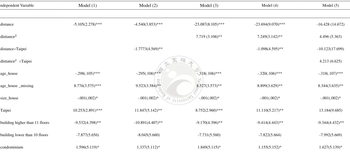
Table 3 shows the effect of the distance to MRT station on housing prices when we
limit the sample to those within 3 km from the MRT stations. Model (1) shows that the
distance to the MRT station, the age of the house, size of the house, and location of the
house are all significant determinant of housing prices. Distance to MRT stations has a
negative effect on housing prices, which means that when the distance increases, the
housing prices decrease and this result consists of the previous studies. The results suggest
that when the distance increases by 1 km; the housing prices decrease by $NT50,000/ping
Model (2) shows the different impact of the distance to MRT station on housing prices
in Taipei and Kaohsiung. The result indicates that when the distance increases by 1 km,
the housing prices in Taipei decrease by an additional $NT17,773 per ping, as opposed to
Kaohsiung.
Based on Model (3), Distance2 is statistically significant and the result indicates that
the rate of the decrease in housing prices declines as the distance increases. Model (4)
is our major model. When we have partial housing prices over partial distance, the
17
Table 3. The Effect of Distance on Housing Prices: Distance to MRT station ≦ 3 km
Independent Variable Model (1) Model (2) Model (3) Model (4) Model (5)
distance -5.105(2.278)*** -4.540(3.853)*** -23.087(8.105)*** -23.694(9.070)*** -16.428 (14.672) distance2 7.719 (3.106)** 7.249(3.142)** 4.496 (5.363) distance×Taipei -1.7773(4.569)** -1.098(4.595)** -10.123(17.699) distance2 ×Taipei 4.213 (6.625) age_house -.298(.105)*** -.295(.106)*** -.318(.106)*** -.320(.106)*** -.318(.107)*** age_house _missing 8.776(3.575)*** 9.523(3.584)** 8.527(3.573)** 8.899(3.629)** 8.344(3.635)** size_house -.001(.002)* -.001(.002)* -.001(.002)* -.001(.002)* -.001(.002)* Taipei 10.253(2.891)*** 11.847(5.142)** 8.752(2.960)*** 11.110(5.217)** 13.184(9.685)
building higher than 11 floors -9.532(4.398)** -10.891(4.407)** -9.170(4.396)** -9.414(4.443)** -9.344(4.432)**
building lower than 10 floors -7.877(5.656) -8.045(5.660) -7.731(5.560) -7.822(5.664) -7.992(5.669)
18
Notes: 2017 = 0, Single-family house = 0, Kaohsiung = 0. Standard errors are in parentheses.
*** Significant at 1% significance level. ** Significant at 5% significance level. * Significant at 10% significance level
Refer to Table 3 (continued)
studio apartment -2.783(6.257)* -3.480(6.255)* -2.079(6.528)* -2.709(6.296)* -2.617(6.316)* storefront 10.581(8.591) 10.661(8.660) 10.489(8.528) 10.469(8.569) 10.103(8.615) commercial building -3.677(7.919) -3.865(7.890) -3.38(7.899) -5.510(7.899) -4.382(8.073) others -5.406(6.846) -4.657(6.858) -5.472(6.856) -5.472(6.856) -5.340(6.872) 2012 4.477(6.376) 4.533(6.384) 3.841(6.385) 4.533(6.384) 3.699 (6.411) 2013 12.048(4.458)** 12.010(4.462)** 11.537(4.459)*** 12.010 (4.462)*** 11.491 (4.464)*** 2014 9.632(4.056)** 9.552(4.906)** 9.513(4.075)** 9.552(4.593)** 9.435 4.098)** 2015 3.276(4.078) 3.238(4.084) 2.839(4.079) 3.238(4.084) 2.722 (4.090) 2016 1.574(4.152) 1.534(4.153) 1.761(4.149) 1.534(4.158) 1.769 (4.156) N 2244 2244 2244 2244 2244 F-value 34.755 33.953 33.670 33.285 30.397 R2 .272 .276 .277 .275 .279
19
prices decrease by $NT119,467per ping in Taipei and decrease by $NT108,487 per ping
in Kaohsiung. The relationship between the distance to MRT stations and housing prices
is a U shape.
Moreover, the interaction term distance×Taipei is negative. It means that the distance
to MRT station in Taipei has a greater impact than that in Kaohsiung. It is because,
compared with Kaohsiung, Taipei has complete MRT systems; thus, people in Taipei are
more dependent on the MRT system. On the contrary, the MRT system in Kaohsiung is
less complete. Therefore, people would choose to ride a scooter instead of taking MRT.
The coefficients of distance, distance2, distance×Taipei and distance2×Taipei in
Model (5) are not statistically significant. This might be the outcome of the small
sample size. When we look at Model (1), the housing prices drop by $NT2,980 if the age
of house increases by one year. As Model (3) shows, when the age of the house increase
one year, the housing prices decrease by $NT3,180. Model (4) indicates that if the age of
house increases on the year, the housing prices drop by $NT3,200 and model (5) shows
that the housing prices decrease by $NT3,180 when the age of house increase one year.
The size of the house also affects the housing prices. All the models suggest that when
the size of the house increases by 10 pings, the housing prices per ping decrease by
20
housing prices in the year 2013 are higher than any other years in our sample, which
suggests that the housing market hit the record high in 2013 in Taiwan.
VI. Conclusions
In this study, we use the transactions data of real estate in Taipei and Kaohsiung from
the Ministry of Interior to test five regression models and estimate the impacts of the
distance to MRT stations on housing prices and test whether this effect is different
between Taipei and Kaohsiung.
The findings are as follows. First, distance to MRT station with 1.5 km and 3 km has a
significant negative impact on housing prices. Furthermore, the rate of the decrease in
housing prices declines as the distance increases. The potential reason might be people
would not choose to take MRT when they live too far away from MRT stations. Second,
the impact of distance to MRT stations on housing prices between Taipei and Kaohsiung
is different. The impact the distance to MRT stations on housing prices in Kaohsiung is
smaller than in Taipei.
Several reasons can explain why distance to MRT stations has a greater effect on
housing prices in Taipei. First, Taipei has more extensive MRT systems, compared with
Kaohsiung. As the result, it is convenient to travel in the city by taking MRT. People
21
in Kaohsiung only cover few districts and as a result, people prefer to ride a scooter
instead of taking MRT.
Second, parking space in Taipei is scarce and the parking fee is high, compared with
Kaohsiung. More importantly, the stricter law enforcement for traffic violations and
illegal parking in Taipei leads people to take MRT. Nevertheless, law enforcement is loose
in Kaohsiung, which fails to encourage people to use public transportation.
Third, the traffic is heavy especially during the rush hours in Taipei. To lower the cost
of commuting, people prefer to take MRT. On the other hand, traffic in Kaohsiung is not
as congested as Taipei. Riding scooter becomes a cheaper option people living in
Kaohsiung.
This paper is our first attempt to examine the effect of the distance to MRT stations on
housing prices. Future research can include Taoyuan MRT system and compare the
differential effect of the distance to MRT stations on housing prices in these three cities.
22 Reference
1. Armstrong, R. J., and Rodriguez, D. A. (2006). “An Evaluation of the Accessibility
Benefits of Commuter Rail in Eastern Massachusetts Using Spatial Hedonic Price
Function.” Transportation 33, no. 1: 21-43.
2. Bajic, V., (1983). “The Effect of a New Subway Line on Housing Prices in
Metropolitan Toronto.” Urban Studies 33, no. 1: 21-43.
3. Benjamin, J. D., and Sirmans, G. S. (1996). “Mass Transportation, Apartment Rent
and Property Values.” Journal of Real Estate Research 12, no. 1: 1-8.
4. Bowes, D. R., and Ihlandfeldt, K.R. (2001). “Identifying the Impacts of Rail Transit
Stations on Residential Property Value.” Journal of Urban Economics 50: 1-25.
5. Chernobai, E., Reibel M., Carney, M. (2011). “Nonlinear Spatial and Temporal
Effects of Highway Construction on House Prices.” Journal of Real Estate Finance
and Economics. 42: 348-370.
6. Coffman, C, and Gregson, M. E. (1998). “Railroad Development and Land Value.”
Journal of Real Estate Finance and Economics. 16, no. 2: 194-204.
7. Damm, D., Lerman S. R., Learner-Lam, E., and Young, J. (1980). “Response of
Urban Real Estate Values in Anticipation of the Washington Metro.” Journal of
23
8. Debrezion, G., Pels, E., and Rietveld, P. (2007). “The Impact of Railway Stations on
Residential and Commercial Property Value: A Meta-analysis.” Journal of Real
Estate Finance and Economics. 35: 161-180.
9. Dewees, D. N. (1976). “The Effect of the Subway Improvement on Residential
Property Values in Toronto”, Journal of Urban Economics. 3: 357-369.
10. Feng, C. M., Tseng, P. Y., and Wang, G. F. (1994). “Impact of Rail Rapid Transit
System on Housing Price in the Station Area.” City and Planning. 21, no. 1: 25-45
11. Debrezion, G., Pels, E., and Rietveld, P. (2007). “The Impact of Railway Stations on
Residential and Commercial Property Value: A Meta-analysis.” Journal of Real
Estate Finance and Economics. 35, Issue 2: 161-180.
12. Hong, D. Y., Lin, C. C. (1999). “A Study on the Impact of Subway System and Road
Width on the Housing Prices of Taipei.” Journal of Housing Studies. 8: 47-67.
13. Kilpatrick, J. A., Throupe, R. L., Carruthers, J. I. and Krause, A. (2007). “The Impact
of Transit Corridors on Residential Property Values.” Journal of Real Estate
Research. 29, no. 3: pp303-320.
14. Tai, K. C. (2011). “The Reexamination of the Impact of Mass Rapid Transportation
on Residential Housing in Taipei Metropolitan.” Department of Land Economics:
24
15. McDonald, J. F., and Osuji, C. I. (1995). “The Effect of Anticipated Transportation
Improvement on Residential Land Values.” Regional Science and Urban Economics.
25, no. 3: 261-278.
16. McMillian, D. P., and McDonald, J. (2004). “Reaction of Prices to a New Rapid
Transit Line; Chicago’s Midway Line, 1983-1999”, Real Estate Economics. 32, no.3:
463-486.
17. Peng, C. W., Yang, S. Y. and Yang, C. H (2009). “The Impacts of Subways on Metropolitan Housing Prices in Different Locations ─ After the Opening of the Taipei Subway System.” Journal of Transportation Planning. 38, no. 3: 275-296.
18. Reibel, M., Chernobai, E. and Carney, M. (2008). “House Price Change and
Highway Construction: Spatial and Temporal Heterogeneity”, paper presented at
Annual Meeting of the American Real Estate Society.
19. Speyer, J. and W. R. Ragas. (1991). “Housing Prices and Flood Risk: An
Examination using Spline Regression.” Journal of Real Estate and Finance
Economics. 4: 395-407.
20. Strawczynski, M. (1998). “Social Insurance and the Optimal Piecewise Linear
Income Tax.” Journal of Public Economics. 69, no.3: 371-388
25
Regression Methods.” The Review of Economics and Statistics. 60, no.1: 132-139.
22. Waddell, P., Berry, B. J. L. and Hoch, I. (1993). “Residential Property Values in a
Multinodal Urban Area: New Evidence on the Implicit Price of Location.” Journal
of Real Estate Finance and Economics. 7: 117-141.