顧客與供應商關係與成本僵固性

國立臺灣大學管理學院會計學研究所 碩士論文

Graduate Institute of Accounting College of Management

National Taiwan University Master Thesis

顧客與供應商關係與成本僵固性

Customer-supplier Relationship and Cost Stickiness

林杰 Lin, Chieh

指導教授：許文馨 博士 劉心才 博士 Advisor: Hsu, Wen-Hsin, Ph.D.

Liu, Hsin-Tsai, Ph.D 中華民國 105 年 9 月

September, 2016

1

摘要

傳統的成本模型指出變動成本應與銷貨收入成等比例的變動。然而 Anderson et al.(2003)的研究指出許多成本具有僵固性- 成本在銷貨收入上升時的調整幅 度大於當銷貨收入下滑時調整之幅度。本研究調查顧客與供應商關係對於公司成 本結構的影響。實證結果指出，當供應商的顧客集中度越高時，該供應商的成本 結構較不僵固。傳統的顧客與供應商關係理論指出主要顧客較強的議價能力能迫 使供應商保留產能，導致成本僵固。然而我們的實證結果指出，供應商與顧客關 係將使雙方有更密切的資訊交流，供應商與顧客的資訊交流溝通使得供應商能及 時調整產能，因此成本較不僵固。本研究指出供應商與顧客關係應為研究公司成 本結構時應考量之因素。

關鍵字：成本僵固性;顧客與供應商關係;顧客集中度

2

Abstract

Traditional model of cost behavior assumes that cost changes proportionally with sales. However, Anderson et al. (2003) show that costs may behave sticky in the sense that costs increase in response to the increase in sales, but do not decrease proportionately when sales decrease by the equivalent amount. This study investigates whether and how relationship with major customers can affect its cost stickiness. The evidence shows that costs are less sticky for firms which have higher concentrated customer bases. Different from the conventional view, which suggests that major customers may pressure suppliers to retain resources when sales decrease and thus, increase the stickiness of cost, the study finds that suppliers have more information from their customer-supplier relationship through better information transfers along the supply chain. Suppliers are more certain about future demand, thus adjusting their costs accordingly in time. Overall, my study shows the importance of customer-supplier relationship when analyzing a firm’s cost behavior.

Key words: Cost stickiness; Customer-supplier relationship; Customer-base concentration

3

Index

口試委員審定書 ... #

Abstract ... 2

Index ... 3

List of Table ... 5

1. Introduction ... 6

2. Literature Review ... 12

2.1 Cost behaviors ... 12

2.1.1 Average cost and marginal costs ... 12

2.2 Cost stickiness... 13

2.2.1 Definition of cost stickiness and why cost stickiness occurs ... 13

2.2.2 Cost stickiness across different categories ... 16

2.2.3 Explanations associated with the degree of cost stickiness ... 16

2.2.4 Consequences of cost stickiness ... 19

2.3 Literature Review on Supply Chain Relationship ... 21

2.3.1 Customer concentration ... 21

2.3.2 The information transfer across supply chain/customer ... 24

3. Hypothesis Development ... 28

4. Research design and sample selection ... 30

4.1 Measurement of customer concentration ... 30

4

4.2 Research model ... 30

4.3 Sample Selection... 31

4.4 Descriptive statistics ... 32

5. Empirical Result ... 33

5.1 Empirical Result for Main Hypothesis ... 33

6. Additional Analysis ... 39

6.1 Pairs of customers and suppliers ... 39

6.1.1 Sample for testing the association between customer’s sales change and cost stickiness ... 39

6.1.2 Model for testing the association between customer’s sales change and cost stickiness ... 39

6.1.3 Results for testing the association between customer’s sales change and cost stickiness ... 41

7. Conclusions ... 43

References ... 45

Appendix 1 : Variable definitions ... 52

Appendix 2: Models of cost asymmetry ... 53

5

List of Table

Table 1: Descriptive Statistics of test variables in ... 63

Table 2: Correlation table... 64

Table 3: Main result for H1 - SGA... ... 65

Table 4: Main result for H1 – COGS... 66

Table 5: Main result for H1 - OC... 67

Table 6: Descriptive Statistics of test variables in Additional test……….…….68

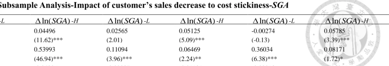
Table 7: Subsample Analysis-Impact of customer’s sales decrease to cost stickiness-SGA..69

6

1. Introduction

The traditional model of cost behavior assumes that costs vary proportionally with sales regardless the sales increase or decrease. However, recent studies document that many costs behave asymmetrically – they fall less with decreases in sales than they rise with equivalent of sales increase (Anderson et al. 2003). This asymmetric cost behavior is labeled as “cost stickiness”, which recognizes the primitives of cost behaviors- resources adjustment costs and managerial decision.¹ When sales decrease, managers tend to retain resources to avoid adjustment cost associate with cutting resources, such as loss of disposal on equipment and severance payment to laid-off employees. In contrast, when sales increase, managers acquire additional resources to meet the demand. When managers are uncertain about future demand, they tend to retain resources in order to lower the adjustment costs of reduce resources or restore resources until they are more certain about the future demand.

Prior studies analyze how the degree of cost stickiness varies with the interaction between managerial decision and adjustment costs and provide economic, agency, and behavioral explanations for cost stickiness. For example, the seminal paper on cost stickiness by Anderson et al. (2003) documents that stickiness of SG&A costs is positively associated with resources adjustment costs. Since adjustment costs tend to be higher when SG&A cost activities rely more on assets owned and people employed than on materials and services purchased by a company, the degree of stickiness increases with the asset intensity and employee intensity of a company. Likewise, using the employment protection legislation (EPL) provision in 19 OECD countries as a proxy for adjustment costs, Banker et al. (2013) find that firms in stricter EPL countries demonstrate greater

1 Costs are “anti-sticky” if they increase less in response to sales increases than they fall when sales decrease (Weiss 2010).

7

cost stickiness. Another stream of studies focuses on agency explanations. Specifically, empire building incentives motivate managers to keep excess resources, resulting in greater cost stickiness (Chen et al. 2012) while earnings management incentives motivate managers to cut down the costs to improve earnings performance, resulting in lower cost stickiness (Dierynck et al. 2012; Kama and Weiss 2013; Banker and Fang 2013). In addition, managerial optimism and pessimism could reflect either rational expectations on future sales based on available information (e.g., cost exhibits greater stickiness during the periods of macroeconomic growth, Anderson et al. 2003) or managerial psychological biases. Thus, some studies also provide the behavioral explanations (Chen et al. 2013;

Qin et al. 2015).

Although many studies examine the factors that may affect cost behavior, little has examined the effect of customer-supplier relationship on cost behavior. Chang et al. (2015) find that there is negative relationship between customer concentration and cost elasticity but the effect of customer-supplier relationship on cost stickiness is still unknown. I complement prior research by investigating the link between cost stickiness and customer-supplier relationship. On the one hand, conventional view of customer-supplier relationship highlights on the bargain power of buyers. This view emphasizes that buyer power exists when suppliers depend on a concentrated set of buyers and major customers have the power to push their dependent suppliers to lower the prices, extend credit period, carry extra inventories, etc (e.g., Porter 1974). Gosman and Kohlbeck (2009), for example, suggest that as sales to major customer increase, the buyer power enables major customers to set the price and extend payment period. They therefore find that suppliers’ gross margins and return on assets decrease with the increased sales to major customers.

Consistent with the bargain power argument, in order to keep the relationship with major

8

customers and for fear of losing them, suppliers are likely to retain their capacity even when sales decrease, reflecting cost stickiness.

On the other hand, research on relationship marketing and operations management provides an alternative view that, suppliers with concentrated customer bases achieve better efficiencies by mutual collaboration on marketing and advertising efforts and more effectiveness of selling expenditures (e.g.,Cowley 1988; Kalwani and Narayandas 1995).

Major customer relationship also fosters information sharing and help suppliers arrange production and working capital more precisely and effectively (e.g., Kalwani and Narayandas 1995; Kumar 1996; Ak and Patatoukas. 2016). Patatoukas (2012), using the mandated disclosure data on major customers required by SEC and SFAS, challenges the conventional view by providing the evidences that suppliers with higher customer concentration are positively associated with higher return on assets and lower selling, general, and administrative (SG&A) costs. Ak and Patatoukas (2016) further find that suppliers with more concentrated customer bases hold fewer inventories for less time and are less likely to end up with excess inventories, as indicated by the lower likelihood and magnitude of inventory write-downs. Suppliers can reduce their demand uncertainty through Vendor-Managed Inventory (VMI), Just-In-Time (JIT) manufacturing, and Collaborative Planning, Forecasting, and Replenishment (CPFR) with their limited number of major customers. Lower uncertainty of future demand gives manager information to make corresponding adjustment on the manufacturing cost. Therefore, costs are likely to be less sticky because managers are more certain about the resource needed in the future and react more sensitively to the change in sales volume in both directions.

Which of the two views of customer-supplier relationship prevails in affecting cost stickiness is an empirical question. By using a sample of U.S. manufacturing firms for

9

the year 1976 through 2015 from Compustat Segment Files, the empirical results provide the evidences that the stickiness of costs is mitigated when suppliers have a concentrated customer base. Specifically, following Patatoukas (2012), I construct a measure of customer concentration (CC) to capture the extent to which a supplier’s customer base is concentrated and investigate the association between customer concentration and cost stickiness. I test on three categories of costs- selling, general, and administrative (SG&A) costs, cost of goods sold (COGS), and operating costs. The results show that for suppliers with more concentrated customer bases, SG&A, COGS, and operating costs are less sticky. Specifically, SG&A (COGS) costs increase on average 0.671(1.043) % when sales increase 1%, while SG&A (COGS) costs decrease 0.527(0.979) % when sales decrease by 1%, which exhibit the stickiness of SG&A (COGS) costs. However, I document that cost are less sticky when supplirs have concentrated customer bases. SG&A (COGS) costs increase 0.200 (0.861) % when sales increase 1%, while SG&A costs decrease 0.444(1.147) % when sales decrease by 1%. Operating costs reflect the similar cost pattern. The results suggest that information sharing and collaboration along customer- supplier chain help suppliers to adjust their costs and resources more precisely, thus reducing the degree of cost stickiness.

This study makes several contributions to the literature. First, I identify customer- supplier relationship as a determinant of cost stickiness. Chang et al. (2014) find that customer concentration level is negatively associated with cost elasticity. I also study the effect of customer concentration on cost structure. However, they do not test whether costs are sticky when suppliers have concentrated customer base. My study fills the gap by showing that customer concentration is negatively associated with cost stickiness. This study provides insight into how the nature of supplier-customer relationship affects

10

supplier’s decision on cost structure. My results suggest that customer concentration is an important determinant of cost structure.

Second, our study contributes to the literature of customer-supplier relationship.

Pandit et al. (2011) note that information externalities are likely to appear between economically related firms. They find that quarterly earnings announcements from customers are positively related to suppliers’ market-adjusted returns. Pandit et al. (2011) provide evidences of information transfers along customer-supplier relationship from the view of capital market. Our study provides new evidence of information transfers from the perspective of cost structure and resource adjustments.

Third, our study contributes to the literature on the impact of customer concentration to supplier firms. Prior literature provides two different views of customer concentration on cost stickiness: bargain power view which argues that major customer has more power to pressure suppliers and therefore force suppliers to retain capacity and bear the costs of operating with unutilized capacity when sales fall and operations managements view which emphasizes that major customers increase information sharing with supplier firms and help suppliers to streamline production when sales decrease, reducing cost stickiness.

Our empirical results support the operations management view by showing that supplier’s costs are less sticky when their customer bases are more concentrated. The results suggest that firms with concentrated customer base adjust their costs timelier because the enhanced information sharing along the supply chain provides supplier firms with more messages about future demand.

Finally, this study also validates the relevance of segment reporting requirement for financial statement analysis. Because costs are fundamental determinants of earnings, understanding cost behaviors and the link between cost and customer-base structure helps investors and analysts with earnings forecasts and stock market valuation.

11

The remainder of this study is organized as follows. Section 2 provides literature review of customer-supplier relationship and cost stickiness. Section 3 develops hypotheses. Section 4 outlines the research design and sample selection. Section 5 documents the empirical findings. Section 6 discusses additional analyses and I conclude in Section 7.

12

2. Literature Review 2.1 Cost behaviors

2.1.1 Average cost and marginal costs

In the conventional model of cost behavior, costs are characterized as either fixed or variable. Changes in variable costs are strictly proportional to the cost driver. However, some studies investigate the complexity between costs and activities and find that costs do not move proportionately to the activity levels. Noreen and Soderstrom (1994) is the first to find that the proportionality hypothesis can be rejected for most of the overhead accounts. Using cross-sectional data from various hospitals in Washington State, they find that most of the overhead accounts are not strictly proportional to activities. They document that on average across the accounts, the average cost per unit of activity overstates the marginal cost by about 40% and in some departments by over 100%. In line with the increasing returns to scale (i.e., economics of scale), average costs overstate marginal costs.

Noreen and Soderstrom (1997) examine the time-series behaviors of overhead cost instead of their cross-sectional behaviors since they suggest that a learning organization does not necessarily repeat the same mistakes and incur the proportional costs to activities and thus overstatement of marginal costs may be more serious as the organization expands over time. They find that more accurate predictions of changes in costs are usually generated by assuming that the cost will not change at all (except for inflation) than by assuming that the cost will change in proportion to change in activity. Using a multi- period regression model, they find that the proportion of variable costs in the hospital overhead accounts is apparently very moderate. They suggest that traditional costing system, which assumes that costs are proportional to activities will grossly overstate

13

relevant overhead costs for decision-making and performance evaluation purpose.

2.2 Cost stickiness

2.2.1 Definition of cost stickiness and why cost stickiness occurs

In addition to the cost behavior of variable and fixed costs, another stream of research proposes the cost behavior that recognizes the role of managers in adjusting committed resources in response to changes in activity-based demand. Noreen and Soderstrom (1997) find that costs are more difficult to adjust when activities decrease because costs increase more sensitively in response to the increase in activity than they fall in response to the decrease in activity.

Building upon findings by these studies, Anderson et al. (2003) label this cost behavior that the magnitude of the increases in costs associated with an increase in volume is greater than the magnitude of the decrease in costs associated with an equivalent decrease in volume as ”sticky”, and establish an empirical model to test this cost behavior. In their study, they propose the following model:²

, , ,

0 1 2 ,

, 1 , 1 , 1

&

log log * _ * log

&

i t i t i t

i t

i t i t i t

SG A Revenue Revenue

Decrease Dummy

SG A   Revenue  Revenue 

  

     

   

     

     

(1)

This model provides the basis for the test of stickiness of SG&A costs. The model is written in ratio to improve the comparability of the variable across firms, and in logarithmic form to reduce the effect of potential heteroskedasticity problem. In this model, the coefficient



₁ measures the percentage increase in SG&A costs with a 1 % increase in sales revenue. The value of Decreased_Dummy is 1 when revenue decreases between period t-1 and t, and 0 otherwise. Therefore,



₁ +



₂ measures the percentage

2 Anderson et al. choose SG&A costs as their major interest because "SG&A cost can be meaningfully studied in relation to revenue activity because sales volume drives many of the components of SG&A costs "(Cooper and Kaplan, 1998, p.341). CFO magazine also did an extensive analysis of SG&A costs in relation to sales revenue in its annual SG&A survey.

14

increase in SG&A costs with 1% decrease in sales revenue. They focus on selling, general, and administrative (SG&A) costs in relation to revenue activity because sales volume will affect many of the elements of SG&A cost. If SG&A costs are sticky, the percentage increase in SG&A costs for an increase in sales revenue should be larger than the percentage decrease in SG&A costs for an equivalent decrease in sales revenue.

Using 7,629 U.S. firms over 1979 to 1998, Anderson et al. (2003) provide empirical evidences that SG&A costs increase on average 0.55% per 1% increase in sales but decrease only 0.35% per 1% decrease in sales. They contend that this kind of sticky cost is mainly derived from the effects of adjustment cost and uncertainty of future demand during periods of rising and falling corporate activities. Cost stickiness occurs as managers deliberately adjust the resources committed to activities. When demand increases, managers commit more resources to meet additional sales. When demand falls and there is uncertainty about future demand and thus, managers may purposely postpone reduction in committed resources until they are more certain about the permanence of a decline in demand. Thus, cost stickiness occurs if managers deliberately retain unutilized resources rather than incur adjustment costs to remove committed resources and to replace the resources as the demand restore. Yasukata and Kajiwara (2011), using the data from Tokyo Stock Exchange, provide evidence that cost stickiness is the result of deliberate decision of managers. They use managers’ sales forecasts as a proxy for managers’ prospect of future sales and find that current level of cost stickiness is associated with the prospect of future sales. Subramaniam and Weidenmier (2003) also show that cost stickiness is the result of managers’ asymmetrical response to large demand changes. They argue that managers will expand capacity of the firm by changing the firm’s committed resources when revenue increases by more than ten percent. However, when revenue decrease by more than ten percent, managers may not want or able to

15

change firm’s capacity, causing cost stickiness.

Besides the U.S., cost stickiness is also found in other countries. For example, Calleja at al. (2006) use a sample of US, UK, French, and German stock market to compare the sticky behavior of operating costs in different countries. They find that cost behaviors of firms from the four countries have some common characteristics: costs are sticky but are, in general, less sticky when aggregated over longer periods and when firms suffer larger declines in revenues. They also find that costs of French and German firms are stickier than cost of US and UK firms. They contend that the result is attributable to the differences in systems and managerial oversight.

Some researchers look for the evidences of sticky costs across industry levels. For example, Subramanian and Weidenmier (2003) find that there are inter-industry differences in the cost stickiness behavior of SG&A and COGS costs as well as in the determinants of sticky behavior. They examine the cost stickiness for four different industries: manufacturing, merchandising, service, and financial services. The results show that manufacturing is the “stickiest” industry because of high level of fixed asset and inventory, while merchandising is the “least sticky” due to its highly competitive environment. The other two industries do show some level of stickiness where interest expenses drive stickiness in the financial industry and employee and inventory intensity drive stickiness in the service industry. In addition, merchandise and service firms adjust their cost quickly in response to change in sales revenue due to their low level of fixed asset and the use of temporary help.

Balakrishnan and Gruca (2008), using the data relate to 189 general hospitals from Ontario from 1986 to 1989, investigate inter-departmental variation in cost stickiness They find that costs are sticker in services deemed more central to the hospital’s mission.

They argue that hospital administrators are unwilling to trim costs in core activities

16

because of the nature of hospital’s service and because of the adjustment costs associated with changing this capacity. In comparison, it is easier and cheaper to adjust capacity levels in other services. In sum, cost stickiness is a phenomenon that is widely spread across country-level, industry-level as well as department level.

2.2.2 Cost stickiness across different categories

Subsequent studies document that cost stickiness is pervasive and holds across different cost categories. Subramanian and Weidenmier (2003) argue that due to lack of authoritative guidance, the component of SG&A in one company could be assigned to cost of goods sold in another company. Thus, they examine the stickiness of SG&A, cost of goods sold, and total cost. The results show that SG&A, cost of goods sold, and total cost are sticky across different industries. Calleja et al. (2006), using the sample of four countries from Thomson Banker One, find that operating costs are generally sticky across these countries. They find that in their sample, operating costs increase by 0.97% to 1%

of sales increase, but decrease by only 0.91% to 1% of sales decrease. Dierynck et al.

(2012) find that managers of firms that reporting small profit focus on firing employees who are low cost to fire, while managers of firms that reporting healthy profits fire fewer employees in order to protect their reputation. Instead, those who report healthy profits reduce costs by changing the number of hours that employees work. The results suggest that firms which have incentives to manage earnings upward engage in real earnings management by cutting the labor costs. Thus, firms that meet or beat the zero earnings benchmark show less cost stickiness.

2.2.3 Explanations associated with the degree of cost stickiness

Some studies of cost stickiness try to find the factors associated with the degree of cost stickiness, overall, including (1) economic explanations: a. the magnitude of adjustment costs b. managerial expected future demand c. current unutilized capacity

17

carried from prior periods (2) managerial incentive (agency) explanations: a. incentives to build empires b. incentives to meet earnings targets and (3) behavioral explanation.

2.2.3.1. Economic explanations

Anderson et al. (2003) find that when asset intensity and employee intensity are higher, the degree of cost stickiness increases since the adjustment costs tend to be higher for firms that rely more on asset owned and people employed than materials and services purchased by company. In line with the notion that the degree of cost stickiness reflects the magnitude of adjustment costs, Balakrishnan et al. (2014) show that the asymmetric behavior of costs is conditional on the proportion of fixed costs over the total costs, where the fixed costs cannot be adjusted quickly enough in response to demand shocks.³ Likewise, Banker et al. (2012), using employment protection legislation (EPL) provisions in 19 OECD countries as a proxy for larger labor adjustment costs find that firms in these countries show greater cost stickiness. The empirical result supports the theory that cost stickiness reflects the deliberate resource commitment decision of managers in the presence of adjustment costs.

Facing uncertainty on future demand, managers deliberately adjust committed resources, resulting in cost stickiness (Anderson et al. 2003; 2014). In line with this argument, Anderson et al. (2003) document that cost stickiness declines with the aggregation of periods since managers better assess the permanence of a change in demand and the adjustment costs become smaller than the cost of retaining unutilized resources. Chen et al. (2012) document that a lower degree of SG&A cost stickiness in firms experiencing negative demand shocks in two consecutive years. Because managers are more likely to consider fall in demand to be permanent when sales decrease in two

3Balakrishnan et al. (2014) suggest that in Anderson’s model, changes in cost should be scaled by sales rather than total costs in order to control for the effects of fixed costs.

18

consecutive years and downsize the capacity accordingly.

In addition, Balakrishnan et al. (2004) extend Anderson et al. (2003) and find that capacity utilization may affect the manager's response to a change in activity levels. They argue that manager’s response to a decrease in activity levels is smaller (larger) than that for an increase only when capacity is currently strained (in excess).

2.2.3.2. Agency explanations

Some studies attribute cost stickiness behavior in part to agency problem. For example, Chen et al. (2012) show that cost asymmetry behavior is positive associated with agency problem. Based on the empire building and the downsizing literature, they argue that managers’ incentives to grow a firm beyond its optimal size or to maintain unutilized resources for their personal benefit induce cost stickiness. They also find that effective corporate governance can mitigate the association between agency problem and the degree of cost stickiness since better corporate governance may restrain managers’

incentives to foster their own interests at the expense of the shareholders. On the other hand, Kama and Weiss (2012) find that managers are more likely to cut down on slack resources to save costs when they face incentives to avoid losses or earning decreases, or to meet analyst earnings forecasts. These deliberate adjustments significantly moderate, rather than increase, the degree of cost stickiness. Dierynck et al (2012), using a sample of private Belgium firms, show that managers meeting or beating the zero earnings benchmark increase labor costs to a smaller extent when activity increases and decrease labor costs to a larger extent when activity decreases. Firms that report small profits show cost symmetry because they choose to fire employees, while firms that report small loss or large profits choose to reduce hours of work by employees, thus show cost asymmetry.

2.2.3.3. Behavioral explanations

Based on the psychology literature, Chen et al. (2014) argue that overconfident CEO

19

are more likely to overestimate future demand and therefore less likely to cut SG&A costs when sales decline. Using a sample of S&P1500 firm between year 1992 and 2011, they find that SG&A cost stickiness increases with the degree of CEO overconfidence.

2.2.4 Consequences of cost stickiness

Another strand of cost behavior literature analyzes the properties and consequences of cost stickiness. Banker and Chen (2006) demonstrate that when a time-series earning forecast model incorporates cost stickiness, the accuracy of this forecast model increases substantially over that of other models with only the line items in the financial statement.

In contrast to the conventional view that an increase in the ratio of selling, general, and administrative costs to sales between two periods as a negative signal about future profitability and firm value, Anderson et al. (2007) find that future earnings are positively associated with changes in the SG&A cost ratio in periods in which revenue declines.

Anderson et al. (2007) suggest that the expectations formed by capital market participants are consistent with traditional symmetric cost model as a measure of operating efficiency.

Abnormal returns may be earned on by going long on firms with high increases in the SG&A cost ratio (and short on firms with low increases in the SG&A cost ratio) in revenue-declining periods.

Some studies investigate analyst forecasts. For example, Weiss (2010) documents that firms with stickier cost behavior have less accurate analyst earnings forecasts than firms with less sticky cost behavior. He argues that stickier costs result in a smaller cost adjustment when activity levels decrease and therefore costs can be saved is lower. Lower cost saving leads to a greater decrease in earnings, increasing the variability of the earnings distribution and, therefore, less accurate earnings forecast. Weiss (2010) further find that firms with stickier costs have lower analyst coverage. Weiss’s findings indicate that firms’ cost behavior affects analysts forecast accuracy and coverage and thus capital

20

market. Further, Kim and Kinsey (2010) argue that because of the difficulty in obtaining internal cost data that contains different cost items and cost drivers, analysts, using proportionate cost model, imperfectly adjust cost behavior, resulting in systematic errors in their earnings forecasts. Weiss (2010) also find a weaker market response to earnings surprises for firms with stickier cost behavior, suggesting that investors recognize cost stickiness to some extent and aware that earnings predictability decreases and reported earnings provide less useful information for firms with sticky cost structure.

21

2.3 Literature Review on Supply Chain Relationship 2.3.1 Customer concentration

Customer concentration is defined as the relative size of customers that adds to a firm's revenue. A firm shows high level of customer-based concentration when its revenue is largely contributed by its major customer.

From the view of customer-supplier relationship, two types of interdependence affect the relationship: (1) dependence asymmetry and (2) mutual dependence (Gulati and Sytch, 2007). The conventional view on customer concentration focuses on dependence asymmetry. Galbraith (1952) provides a tactic for customers to exercise their power to their suppliers by keeping the suppliers in uncertainty. Suppliers often invest resources to meet major customer's demand, while major customers can alter their order to other suppliers. Thus, suppliers are usually more dependent on major customers. In contrast, mutual dependence suggests that customer and supplier are dependent on each other. The dependence is especially higher when suppliers sell highly specialized products. Mutual dependence makes the cost of changing supplier/customer more expensive for both parties. Cool and Henderson (1998), using French manufacturing data, show that buyer power explains a much larger percentage of the variance in the seller’s profitability than supplier power. They argue that the power in supply chain may come from the relative degree of concentration among suppliers and customers and the relative resources and product dependence among them.

2.3.1.1 Potential cost of customer concentration

Suppliers with concentrate customer bases face serious dependence asymmetry because of larger and more important customers. Larger customers have a greater impact on supplier’s profits and cash flow and larger customers are more likely to attract other

22

suppliers to do business with them. Serious dependence asymmetry provides customers with strong bargain power, which may impose potential costs on suppliers. Specifically, first, strong bargain power of customer may increase suppliers operating risk. For example, Scherer (1970) argues that suppliers may be fear of instant and heavy losses if the customer changes its supplier. The fear provides customer strong bargain power over price and credit terms. Gosman and Kohlbeck (2009) find that as sales to major customer increases, the gross margins and return on asset of supplier decrease. They argue that the increasing buyer power allows buyers to dictate prices from suppliers and to have fewer inventories and extend payment periods. Second, strong bargain power may induce managers to engage in earning management. Raman and Shahrur (2008) documents that firms engage in earnings management in order to show positive and stable earning potential and to induce their suppliers/customers to invest more in relationship-specific investment. They also find that the duration of customer-supplier relationship is shorter when firms engage in earnings management. Third, strong bargain power may induce managers to engage in tax avoidance. Huang et al. (2015) contend that customer concentration is positively associated with tax avoidance. They argue that for firms with a concentrated corporate customer bases, they have higher cash flow risk because loss of major customers could lead to a considerable drop of cash flow. They also have incentive to manage their earnings to enhance the perception of their customer. Since tax avoidance can increase both cash flow and accounting earnings, firms are more willing to engage in tax avoidance.

2.3.1.2 Benefits of customer concentration

The view of operations management provides us another story. Operations management suggests that limited number of major customers enables suppliers to implement some supply-chain practice to reduce their cost and increase efficiency (Ak

23

and Patatoukas, 2016). For example, collaborative planning, forecasting, and replenishment (CPFR) can enable collaborative supply and demand planning. Under CPFR, supplier will set up an information system with major customer to exchange demand forecasts. Such system can reduce demand uncertainty and thus, reduce inventory uncertainty. A limited number of major customers may also enable suppliers to adopt just-in-time (JIT) manufacturing. Under JIT manufacturing, suppliers can produce their products in small batches, therefore inventory level is reduced (Balakrishnan et al, 1996).

The key point of JIT is coordination with customers, but the coordination cost is high.

Suppliers with few major customers may enjoy lower coordination cost in ordering, scheduling, production, and delivery. Overall, the view of operations management suggests a positive association between customer concentration and efficiency.

Patatoukas (2012) contends that suppliers with more concentrated customer bases spend less on selling, general and administrative (SG&A) expenses per dollar of sales and hold lower inventory. These suppliers also enjoy higher turnover rate of current and non- current assets and shorter cash conversion cycles. He argues that these benefits are due to the increased information sharing and improved production coordination along the supply chain. Improved coordination can help these suppliers to reduce redesign costs and to avoid delay in product development. Ak and Patatoukas (2016) show that manufacturers with more concentrate customer bases have lower inventory holding and shorter inventory holding period. They argue that in operations management view, a limited number of major customers might mitigate demand uncertainty, therefore increasing inventory efficiency. Kalwani & Narayandas (1995) indicate that suppliers who maintain long-term relationship with few customers do not come with a loss in the rate of sales growth overtime. They argue that although the customers may have higher bargain power, these suppliers can still achieve the same level of growth and better profitability by

24

improving inventory utilization and reducing selling, general, and administrative overhead cost.

Irvine et al. (2016) show a dynamic relationship life-cycle of supplier-customer links.

They find a negative association between customer-based concentration and profitability in the early stage of the supplier-customer relationship. However, as the relationship matures, the association between customer-based concentration and profitability becomes positive. They explain that in the early stage of the relationship, suppliers make greater customer-specific SG&A investment in order to earn higher profit in the future. These customer-specific investment increases fixed SG&A expense and therefore, higher operating leverage. As the relation matures, suppliers with higher level of customer concentration enjoy higher operating profit and lower operating risk.

2.3.2 The information transfer across supply chain/customer

2.3.2.1. Auditor perspective

Information transfer along supply chain has some effect on auditors. Krishnan et al.

(2015) find negative relation between customer-base concentration and audit fees. They argue that major customer relationships may enable suppliers to reduce their operating complexity; lower operating complexity for more dependent suppliers would imply lower audit complexity, reducing audit efforts and thus, leading to lower audit fees. They also contend that the audit quality is not impaired because of lower audit fees. They find that suppliers who share the same auditor with at least one of their major customers enjoy additional audit fee discounts, and these suppliers are less likely to experience restatements. These suggest that a positive link between audit quality and major customer dependency. Chen et al. (2015) further find that audit fees are negatively associated with the major buyer-related supply chain knowledge. They show that auditors with more

25

knowledge of supply chain provide more discounts on audit fees to their clients when the major customer is also the auditor’s client. They argue that for audit firms that have engaged the client’s supply chain partners, these audit firms have better understanding of the client’s industry. The audit firms are expected to better evaluate the client’s key accounting figures since these numbers are close linked to those of the client’s major customer, resulting in higher audit quality, therefore the auditor can command fee premium.

2.3.2.2. Stock market perceptive

Many studies have documented evidences on the market reactions to the information along the supply chain. Olsen and Dietrich (1985) give the first evidence that information disclosures made by retailers may affect the security prices of supplier firms. They find that suppliers with a relatively larger proportion of sales to a specific retailer show a relatively larger change in price after the retailer’s monthly sales announcement. They argue that investors may revise their expectation of the sales level of supplier firms after the announcement, and that provides us evidence on vertical information transfers between customers and suppliers.

Pandit et al. (2011) provide further evidence that the degree of transfer of a customer’s quarterly earnings announcement to suppliers’ security returns is positive related to the strength of the economic bond between the suppliers and customers, seasonal changes in the customer revenue and cost of goods sold, the level of macroeconomic uncertainty, and the informativeness of the announcement. They contend that for suppliers that sell large portion of sales to a major customer, information provided by customer’s earning announcement can alter investors’ expectation about the supplier’s cash flows and future earnings. Guan et al. (2015) show that analysts who follow a

26

covered firm’s customer will more accurately forecast the supplier firm’s earning than those who do not. They also find that although both types of analysts respond to customer firm’s earning announcement, those who follow major customer exhibit better forecast accuracy. They argue that the stronger the economic link between suppliers and customers, the greater will be information complementarily between them; therefore increase their forecast accuracy as result.

Cohen and Frazzini (2008) find return predictability across economically linked firms. They give an example of Callaway and Coastcast to show that it is investors’

inattention to company link that provide significantly predictable returns across customer- supplier firms. Investors ignore publicly available information about economically links when they know there is a shock to one firm; thus the stock price of related firms will adjust with a lag to the shock of related firms, leading to predictable returns. Shahrur et al. (2010), using international data across 22 developed countries, show that the return of customer industries leads the return of supplier industries. Their finding is consistent with the view of Cohen and Frazzini (2008) that stock price does not totally reflect publicly available information about economically linked companies. Hertzel et al. (2008) show that financial distress and bankruptcy affect a filing firm’s suppliers. They find that during customers’ bankruptcy filing and pre-filing distress period, suppliers’ abnormal returns are, on average, significantly negative. This effect is more severe when the customers’

rival appears to experience contagion. They explain that suppliers may have fewer opportunities to switch to different customers when the whole industry impairs, and the supplier may have economic relations with rivals of customer that also suffer. They also examine on the filing firm’s customer and find little evidence of this effect.

27

2.3.2.3. Debt market perspective

Some studies talk about the association between customer-supplier relationship and loan contract. Kim et al. (2015) find that for suppliers whose major customers have a higher weighted-average return on asset, these suppliers enjoy lower rate, longer maturity, and fewer covenants for their loans. This is more pronounced when the supplier has no prior lending relationship with the lead banks and when the economic tie between supplier and major customer is stronger. Customers with poor performance are more likely to fail to pay to their suppliers, and poor performance is likely to lower future demand for supplier’s products or service. This would affect supplier’s future cash flow and increase future default risk. They suggest that banks do take customer’s earning performance into account when having contract with the supplier firms, and the effect varies with the strength of customer-supplier relationship. Cen et al. (2015) argue that the reputational effects of long-term supplier-customer relationship are potentially spill over to other markets. They find that suppliers who have a long-term relationship with customers, these suppliers’ loan spreads are lower and enjoy looser covenants on bank loans. They argue that firms that have long-term relationship with major customers are interpreted by banks as a certification of higher product quality, lower default risk, and higher operation stability than other firms in the same industry.

28

3. Hypothesis Development

I expect that customer-based concentration will have impact on cost stickiness. From the view of bargain power, major customers have the power to pressure their dependent suppliers to keep a high level of product availability and retain relationship-specific investments when sales decrease. Suppliers often involve relationship-specific investments in a supplier-customer relationship (Raman and Shahrur 2008), and firms with higher customer concentration make greater relationship-specific investment (Irvine et al. 2016). Such investments are specific to a particular customer in order to meet customers’ need, and the value of investments is lower outside the relationship. As supplier’s sales decrease, major customers have the bargain power to pressure their dependent suppliers to remain their capacity when they expect the possibility of recovery of demand in the future. Suppliers are willing to keep their capacity in order to keep this relationship. The pressure would be more pronounced when the suppliers depend on few major customers.

On the other hand, a more concentrated customer base can increase efficiency through increased information sharing and enhanced production coordination and inventory managements (Patatoukas. 2012). Increased information sharing provides more information to suppliers; thus supplier’s managers are less likely to retain resources when sales decrease since they are more certain about future sales. As Patatoukas (2012) notes, suppliers with concentrated customer bases have better working capital management because of better information sharing and production coordination. Better information sharing along supply chain can help reduce the bullwhip effect since the information asymmetry is reduced. These suppliers also enjoy lower redesign costs. From the view of operations management, the relationship with few major customers allows suppliers to implement some supply-chain practices that can reduce demand uncertainty. (Ak and

29

Patatoukas. 2016). A set of technology-enabled standards such as collaborative planning, forecasting, and replenishment (CPFR), provide a roadmap for enabling collaborative demand and supply planning and execution process. This requires both suppliers and customers to set up system to exchange their information such as demand forecast (Ren et al. 2010). Enhanced information exchange enables suppliers to make a better decision whether to retain resources when sales decrease because the uncertainty of demand is reduced.

In sum, as the link between cost stickiness and customer concentration is ex ante unclear, I state my hypothesis in null form:

H1: There is no association between cost stickiness and customer concentration.

30

4. Research design and sample selection 4.1 Measurement of customer concentration

To capture the extent to which a supplier’s customer base is concentrated, I create variable of customer concentration. I follow Patatoukas (2012) to create my primary measure of customer concentration ( CC ) using the following formula:

2

1

it

J

ijt

j it

Sales

CC ijt

Sales



 

  

 



⁽²⁾

where

Sales

_ijt represents firm

i

’s sales to customer j in year

t

and

Sales

_it

represents total sales for firm

i

in year

t

. Patatoukas (2012) implements Herfindahl- Hirschman index to construct the measure of CC . The measure CC captures two elements of customer concentration: the number of major customer with which the firm interacts and the relative importance of each major customer in the firm’s annual sales.

CC ranges from 0 to 1, with higher value indicates suppliers with more concentrated

customer bases and vice versa.

4.2 Research model

Following the methodology proposed by Banker et al. (2014), I investigate the association between customer concentration and cost stickiness using the regression of following form:

. 0 1 . 2 . 3 . 4 . .

5 . . 6 . . 7 . . .

8 . 9 . 1

( ) ( ) *

+ ( ) * * ( ) * *

i t i t i t i t i t i t

i t i t i t i t i t i t i t

i t i t

ln(Cost) ln Sales CC Dec ln Sales CC

ln Sales Dec CC Dec ln Sales CC Dec GDPGrowth Size

    

  

  

       

   

   _{0 . 11 . 12 . .}

13 . . 1 19 1 19 .

+ * ( )

+ * ( ) * ( )

i t i t i t i t

i t i t i t

ASINT EMPINT ASINT ln Sales

EMPINT ln Sales IndFE IndFE ln Sales

 

  _ _

 

 









(3)

where ln(Cost) is the log-change in costs for a firm from year t - 1 to year t.

Following Chang et al. (2015), I use three different specifications of the ln(Cost)

term: selling, general, and administrative costs (SGA), cost of goods sold (COGS), and

31

total operating costs (OC).ln Sales( )is defined as the log-change in sales for a firm between year t-1 and year t. Dec is a dummy variable that take the value of 1 when sales decrease between year t-1 and t, and 0 otherwise. CC is the measure of customer concentration, calculated as in Equation (1). GDPGrowth refers to the log-change in Gross Domestic Product from year t-1 to year t. Size is defined as the natural log of sales for a firm in year t. I include GDPGrowth and Size as control variables. I expect the coefficient on GDPGrowth and Size to be positive because costs are more sensitive to change in sales and because larger firms have lower adjustment costs. I also include controls for industry fixed effect (IndFE) as well as interactions between industry indicators andln Sales( ). Following ABJ, I include two variables, ASINT and EMPINT, as proxies to measure the magnitude of adjustment cost. ASINT is asset intensity, calculated for each firm-year observation as total asset divided by sales. EMPINT is employee intensity, calculated for each firm-year observation as the number of employees (EMP) divided by sales. I also include the interactions between these two variables with

( )

ln Sales

 . I expect the coefficients on ASINT and EMPINT to be negative because firms with greater asset intensity have more rigid cost structure and firms with greater employee intensity have higher adjustment cost.

4.3 Sample Selection

I identify customer-supplier relationships using the COMPUSTAT Segment File, which includes data on customer name, type, and revenue contributed to the supplier firm.

The COMPUSTAT Segment File is based on FASB’s and SEC’s requirements that public firms disclose revenue derived from each major customers representing more than 10 percent of their total sales. My sample begins in 1976, which is the first year when major customer data is available and ends in 2015, which is the last year that data is available. I gather other financial information about suppliers and customers from COMPUSTAT.

32

Following Banker et al. (2014), I restrict my sample to manufacturing firms (four digits SIC codes 2000 - 3999). Following Irvine et al. (2016), I remove observations that customers are not identified as company type since government customers are considered as low risk customers. I eliminate observations which supplier sales, SG&A or operating costs are missing. I also exclude observations for which SG&A costs exceed sales because these observations express unusually large commitments of SG&A resources. To control for the potential effect of outliers, I winsorize the data at the top and the bottom 1 percent.

4.4 Descriptive statistics

Table 1 presents the descriptive statistics of variables used in H1. The number of observations is different among variables due to data availability, which leads to different sample size for different variables used in the regression. In this study, although I exclude observations which SG&A costs are missing, I do not require that all cost variables to be jointly available but only those that are required in each test. The average (median) firm in our sample reported sales revenue of $834 ($91) million dollars of sales, $151 ($20) million dollars of selling, general and administrative costs. Note that the mean (median) value of CC, variable that measures cost concentration, is 0.104 (0.051) in our sample, and interquartile range is from 0.017 to 0.131. This shows significant variation in customer-based concentration among supplier firms in our sample. The mean and median of CC is similar to that in Patatoukas (2012) and Chang et al. (2015).

Table 2 present correlations among variables used in my test. Pearson (Spearman) correlation is reported in the upper (lower) part of the table. Sale is highly positively correlated with selected cost variables (SGA, COGS, and OC), which indicates that using sales as cost driver is appropriate. Note that Size is negatively correlated with CC, which can be explained that smaller firms have more concentrated customer bases.

33

5. Empirical Result

5.1 Empirical Result for Main Hypothesis

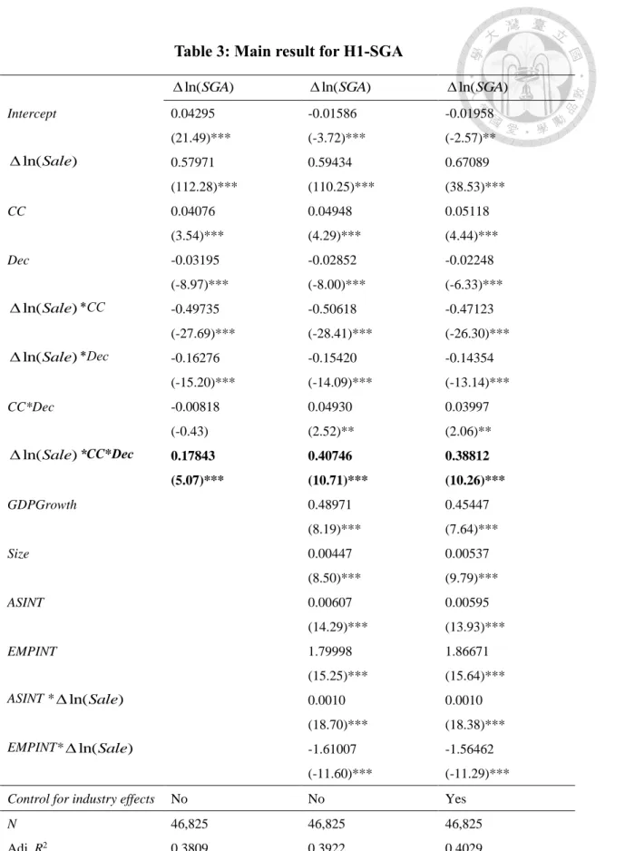
Table 3 through Table 5 shows the empirical results of the overall effect of customer concentration on cost stickiness. Estimates of three different variables of costs, which are SGA, COGS, and OC, are shown in Table 3 through Table 5 with three specifications, respectively. SG&A costs are most commonly used in the literature on cost stickiness since the seminal paper, Anderson et al. (2003). I report the results in Table 3.

First, Column (1) of Table 3 reports the baseline model derived from Anderson et al.

(2013) with the modification that my variable of interest CC is incorporated. Specifically, the coefficient on ∆𝑙𝑛(𝑆𝑎𝑙𝑒) is 0.57971 (t-statistic =112.28), positively significant at the 0.1% level, which is consistent with prior literature that SG&A costs are positively associated with the sales revenue. The estimated coefficient, 0.57971 indicates that SG&A costs increase 0.57 % per 1% increase in sales revenue. The coefficient on

ln(Sale)



*Dec is -0.16276 (t-statistic =-15.20), significantly negative at the 0.1% level,

which is consistent with the results in Anderson et al. (2003) that provides strong support for cost stickiness. The combined value of these two coefficients on ln(Sale) and

ln(Sale)



*Dec is 0.43434, indicating that SG&A costs decreases only 0.43% per 1%

decrease in sales revenue. The fact that both the coefficient on ln(Sale) and the combined value of the two coefficients are both significantly less than one, indicating that SG&A costs are not proportional to changes in sales revenue, even though SG&A cost driver should be closely related to sales. When customer concentration (CC) is incorporated in the model, the coefficient on my variable of interest, CC*∆𝑙𝑛(𝑆𝑎𝑙𝑒)*Dec, is 0.17843 (t-static =5.07), significantly positive at the 0.1 % level. The result indicates

34

that for companies with more concentrated customers, SG&A costs are less sticky when sales decrease. Column (2) of Table 3, I report the results with control for economic explanations that may affect the degree of cost stickiness based on the prior literature.

Likewise, the coefficient on ∆𝑙𝑛(𝑆𝑎𝑙𝑒) is 0.59434 (t-statistic =110.25), positively significant at the 0.1% level, indicating that SG&A costs are positively associated with the sales revenue. The estimated coefficient, 0.59434 indicates that SG&A costs increase 0.59 % per 1% increase in sales revenue. The coefficient on ln(Sale)

*Dec is -0.15420

(t-statistic =-14.09), significantly negative at the 0.1% level, which provides strong support for cost stickiness. The combined value of these two coefficients on ln(Sale) and ln(Sale)

*Dec is 0.44014, indicating that SG&A costs decreases only 0.44% per

1% decrease in sales revenue. When customer concentration (CC) is incorporated in the model, the coefficient on my variable of interest, CC*∆𝑙𝑛(𝑆𝑎𝑙𝑒)*Dec, is 0.40746 (t-static

=10.71), significantly positive at the 0.1 % level. The result provides strong support for the notion that for companies with more concentrated customers, SG&A costs are less sticky when sales decrease. Regarding the control variables, the coefficient on

GDPGrowth is 0.48971(t-static=8.19) significantly positive at the 0.1% level, which is

consistent with prior literature that macroeconomic environment is promising; firms may have sales growth and increase their investment in the production process. The coefficient on ASINT * ln(Sale) is 0.0010 (t-static=18.70), significantly positive at 0.1%, consistent with prior literature. The result provide strong support for the notion that when asset intensity is higher, the degree of cost stickiness increases since the adjustment costs tend to be higher for firm that rely more on asset owned, such as warehouse, plant, and equipment. The coefficient on EMPINT* ln(Sale) is -1.61007 (t-static=-11.60) negatively significant at 0.1% level. This result is not consistent with the notion suggested by the prior literature that when employee intensity is higher, the degree of cost stickiness

35

should increases since the adjustment costs tend to be higher for firm that rely more on people employed whom are not easy to removed.

Column (3) of Table 3 reports the results with full control variables with indicator variables for industry fixed effects in order to it control for the potentially unobserved industry specific factors that are related to cost behaviors. The results are very alike.

Specifically, the coefficient on ∆𝑙𝑛(𝑆𝑎𝑙𝑒) is 0.67089 (t-statistic =38.53), positively significant at the 0.1% level, which indicates that SG&A costs are positively associated with the sales revenue. SG&A costs increase 0.67 % per 1% increase in sales revenue.

The coefficient on ln(Sale)

*Dec is -0.14354 (t-statistic =-13.14), significantly

negative at the 0.1% level, which is consistent with the presence of cost stickiness. The combine value of these two coefficients on ln(Sale) and ln(Sale)

*Dec is

0.52735, indicating that SG&A costs decreases only 0.52% per 1% decrease in sales revenue. The fact that both the coefficient on ln(Sale) and the combined value of the two coefficients are both significantly less than one, indicating that SG&A costs are not proportional to changes in sales revenue, When customer concentration (CC) is incorporated in the model, the coefficient on my variable of interest,

CC*∆𝑙𝑛(𝑆𝑎𝑙𝑒)*Dec, is 0.38812 (t-static =10.26), significantly positive at the 0.1 %

level. The result indicates that for companies with more concentrated customers, SG&A costs are less sticky when sales decrease. The coefficients on the control variables are similar as we reported in Column (2) of Table 3.

Overall, my results reported in Table 3 cross three specifications show that although consistent with prior literature that SG&A cost behavior reflect a “sticky” pattern, that SG&A as a variable component of total costs decrease less with a sales decrease than they increase with an equivalent sales increase, when companies with more concentrated customers, SG&A costs are less sticky when sales decrease. The results support the

36

operations management view that suppliers with concentrated customer bases achieve better efficiencies by mutual collaboration and information sharing.

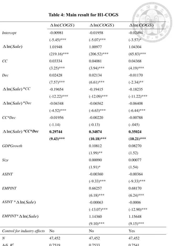
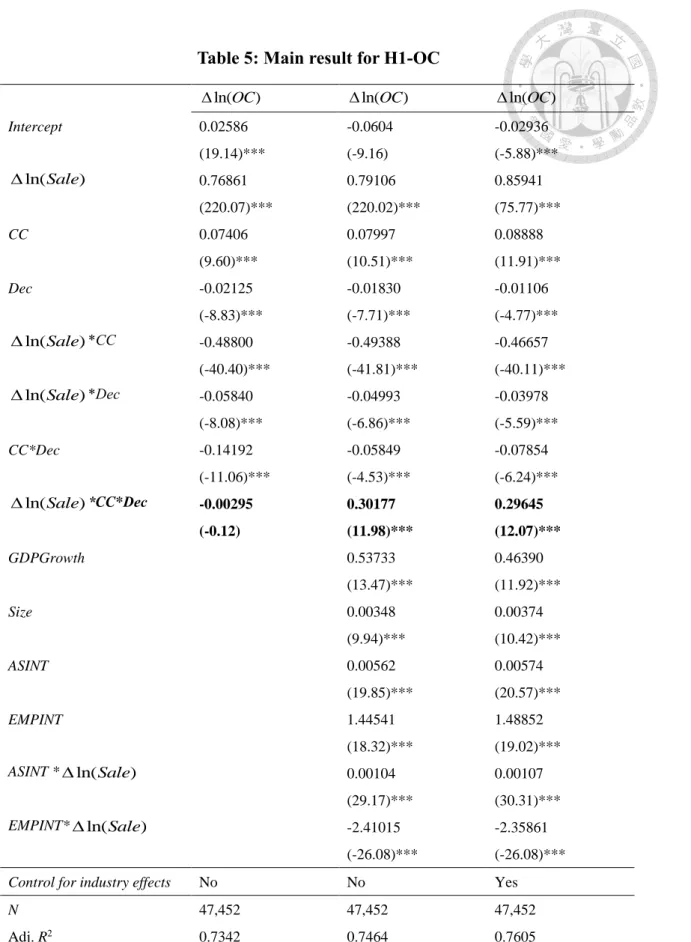
Based on argument by Subramanian and Weidenmier (2003) that due to lack of authoritative guidance, the component of SG&A in one company could be assigned to cost of goods sold in another company, I also investigate the stickiness of cost of goods sold (GOGS) and total operating cost (OC) and report the results in Table 4 and Table 5 respectively.

Column (1) of Table 4 reports the baseline results of Anderson et al. (2003) model with the extension of my variable of interest (CC). The coefficient on ∆𝑙𝑛(𝑆𝑎𝑙𝑒) is 1.01948 (t-statistic =219.16), positively significant at the 0.1% level, which is as expected that cost of goods sold (COGS) are highly correlated to the sales revenue. The estimated coefficient, 1.01948 indicates that COGS increase almost 1 % per 1% increase in sales revenue. The coefficient on ln(Sale)

*Dec is -0.04348 (t-statistic =-4.52), significantly

negative at the 1% level, which is consistent with the notion that COGS is sticky. The combined value of these two coefficients on ln(Sale) and ln(Sale)

*Dec is 0.976,

indicating that COGS decreases only 0.976 % per 1% decrease in sales revenue. When customer concentration (CC) is included in the model, the coefficient on my variable of interest, CC*∆𝑙𝑛(𝑆𝑎𝑙𝑒)*Dec, is 0.29744 (t-static =9.43), significantly positive at the 0.1

% level. The result suggests that for companies with more concentrated customers, COGS is less sticky when sales decrease. Column (2) of Table 4, I report the results with control variables for factors that may affect the degree of cost stickiness. Likewise, the coefficient on ∆𝑙𝑛(𝑆𝑎𝑙𝑒) is 1.00977 (t-statistic =206.52), positively significant at the 0.1% level, indicating that COGS are positively associated with the sales revenue. COGS increases nearly 1 % per 1% increase in sales revenue. The coefficient on ln(Sale)

*Dec is -0.06562 (t-statistic =-6.63), significantly negative at the 0.1% level, which