Patent Rights Protection and High-Tech Exports:
New Evidence from Taiwan
✽Judy Hsu
✽✽Associate Professor, Department of International Business, Feng Chia University
Jong-Rong Chen
Professor, Graduate Institution of Industrial Economics, National Central University Joint Appointment Research Fellow, RCHSS, Academia Sinica
Adjunct Research Fellow, PERC, College of Social Sciences, National Taiwan University
ABSTRACT
An array of literature empirically examines the impact of patent rights (PRs) protection on international trade, but most studies employ the traditional gravity model to estimate and ignore firm-level behavior. Helpman, Melitz and Rubin- stein (2008) propose a two-stage, non-linear least squares estimation procedure (the HMR model) to correct potential biases embodied in the gravity estimation of trade flows, which decomposes the impact on trade volumes of all trade resis- tance measures into their extensive and intensive margin components. Yet, Santos Silva and Tenreyro (2015) suggest that the HMR model is incorrectly specified and propose the Poisson pseudo maximum likelihood (PPML) methodology to solve heteroscedasticity. Utilizing the HMR model and the PPML method, this paper empirically investigates how differences in PRs protection may influence Taiwan’s semiconductor exports to 119 destination countries from 1995 to 2010.
Our results support the effectiveness of an importing country’s patent harmoni- zation in stimulating importation of high-tech goods from Taiwan.
Key Words: patent rights, high-tech, semiconductor, export, HMR, PPML
✽ We would like to thank three anonymous referees for their valuable comments and incisive sugges- tions that helped to improve the paper substantially. Financial support from the Ministry of Sci- ence and Technology of Taiwan (grant number: MOST 104–2410–H–035–005) is also gratefully acknowledged. The usual disclaimer applies.
✽✽ Corresponding Author: E-mail: yphsu@fcu.edu.tw Received: May 8, 2018; Accepted: November 12, 2018
©2019 by RCHSS, Academia Sinica. All rights reserved.
I. Introduction
The emergence of global intellectual property rights (IPRs) protection regimes based on the agreement on Trade-Related Intellectual Property Rights (TRIPS) is a subject of considerable debate. Arguments center on the effects of IPRs on inter- national technology generation and transfers, trade performance, FDI flows, and growth. In 1995, the TRIPS agreement, which seeks global harmonization of IPR laws, came into effect. All countries that are members of the World Trade Organi- zation (WTO) are required to follow the TRIPS guidelines to adopt common global laws for protection of intellectual properties as embodied in patents, copyrights, trademarks, and trade secrets. Patent rights (PRs) protection has acquired an important role in the new knowledge-based global economy. Traditionally, devel- oping countries have established weaker regimes that favor technological diffusion through imitation and acquisition from abroad. By contrast, developed countries have long promoted the idea of stronger intellectual property protection throughout the world to improve incentives for private agents to create and advance technology for their own inventors to extract greater returns from their discoveries. Pressure from developed countries and often in conjunction with concessions on opening their domestic product markets to more imports have led many developing countries to begin strengthening their intellectual property systems, particularly on patents.
An ongoing debate over the role of IPRs and international technology diffu- sion can be observed through a variety of formal and informal channels, including trade in goods, foreign direct investment (FDI), international patenting, technology licensing, etc., at the country level. PRs can affect these channels in different ways.
Proponents of less stringent protection suggest that further controls on PRs would harm imitation-cum-innovation development strategies and constitute a barrier to legitimate trade in imitative products. By contrast, proponents of more stringent protection suggest that lax protection distorts natural trading patterns. PRs protec- tion can prevent the product of a manufacturing firm from being imitated by its competitors and protect its economic well-being. However, in the presence of national differences in the IPRs system, the decision made by an exporting firm on a country which its products are shipped to will be distorted. Several empirical studies have considered the relationship between PRs and a particular channel of diffusion (Briggs, 2013; Co, 2004; Deardorff, 1992; Eaton and Kortum, 1996;
Helpman et al., 2008; Hsu and Tiao, 2015; Ivus, 2010; Liu and Lin, 2005; Maskus and Eby-Konan, 1994; Maskus and Penubarti, 1995; Rafiquzzaman, 2002; Smith, 1999; Yang and Maskus, 2001; Yang and Woo, 2006). The outcomes of these stud-
ies are mixed, although stronger evidence can be found for the importance of PRs protection for trade and patenting than for FDI.
Although previous literature has investigated the effects of PRs protection on overall and industry-level bilateral trade flows across countries, most studies employ traditional gravity models to estimate and ignore firm-level behavior (extensive and/or intensive margin changes). In fact, the effect of PRs can be displayed through the variety (i.e., extensive margin) and volume (i.e., intensive margin) of trade.
Helpman, Melitz, and Rubinstein (2008), henceforth HMR, propose a two-stage, non-linear least squares (NLS) estimation procedure to correct the two types of potential bias of the standard gravity model, which are sample selection bias and bias from potential asymmetries in the trade flow between pairs of countries. The model enables insight into a firm’s binary decision to export to a given market based on the continuous decision on the amount of exports, and allows empiricists to determine firm-level decision making behavior while using aggregate country data. The ability to obtain such decomposition is important because in practice, a substantial proportion of trade adjustment occurs at the extensive margin, and obtaining consistent firm-level data with export destinations is nearly impossible for many countries. HMR argues that controlling for extensive margin and sample selection would eliminate bias in the estimation.
However, Santos Silva and Tenreyro (2015) argue that the HMR model is valid only under the dependence on homoscedasticity. They suggest the HMR model is specified incorrectly and casts doubts on any inference drawn from the empirical implementation of the HMR model.1 They propose an econometric solution to the
“zero problem,” which is the Poisson pseudo-maximum likelihood (PPML) estima- tor. The Poisson model commonly used for count data can be applied more gener- ally to non-integer variables and is equivalent to (weighted) non-linear least squares.
The estimator is consistent under weak assumptions, and data need not be distrib- uted as Poisson. Their point is a very general one, whereby the econometric esti- mates of log-linearized models can be misleading because of a particular and nox- ious type of heteroscedasticity.
The influence of stronger PRs protection on the exports of developed countries has not received much attention in the literature. Due to the estimation biases of traditional gravity model, this paper adopts the HMR model and the PPML method accompanied by traditional gravity estimation to examine empirically how differ- ences in PR protection between countries influence the export of a developed coun-
1 They show that HMR two-stage estimator is very sensitive to departures from the assumption of homoscedasticity. However, heteroscedasticity is commonly found in most trade data.
try, such as Taiwan, in a knowledge-based industry, namely the high-tech industry.
The study covers 1995 to 2010 and considers 119 trade partners of Taiwan. The semiconductor industry was chosen mainly because it has been thriving on a soft patent regime followed by Taiwan since 1986 and has become one of the most crucial export-oriented sectors of today. Besides, under the development of a global value chain, the semiconductor trade is usually regarded as a trade of intermediate goods, and thus avoids the double-counting problem often found in the final goods trade.
Moreover, unlike most previous studies using data from the U.S. or European Union, the advantage of using data from Taiwan is that it is a small country with almost no influence on the patent protection policies in other counties. Thus, there is no worry of the potential reverse causality (i.e. the destination country’s protec- tion level might be affected by the trade volume). To the best of our knowledge, this study is the first empirical study on the possible linkage between PRs protection difference and semiconductor exports of Taiwan by using the recently developed HMR model and PPML method. Therefore, this paper can shed light on the related literature by providing a noteworthy exploration of a developed country.
The remainder of the paper is organized in the following way. The next sec- tion reviews briefly the main findings of related literature. In the third section, we present the general empirical methodology and introduce the dataset. The fourth section presents and discusses the empirical findings. The last section concludes.
II. Literature Review
An increasing amount of literature is addressing the factors that contribute to international technology diffusion, such as international trade. International tech- nology diffusion is the process by which technology moves from country to coun- try and is considered to have a significant effect on country-income levels. Obtain- ing technology from another country increases productivity growth, especially for poorer countries that invest less in R&D than more developed nations (Keller, 2004).
Technology transfers between countries are at the heart of this issue, and consider- ation of how PRs influence international trade and technology diffusion is worth- while. The cost savings from forgoing the R&D process can lead to lower prices for the foreign producer, making it difficult for the original intellectual property creator to compete. In this way, the lack of consistent PRs across countries could hamper international technology diffusion by reducing trade in goods. Therefore, increased understanding of how PRs influence tradeflows is essential to the devel- opment of a constructive trade policy that benefits all countries involved.
Empirical studies on the PRs-exports relationship began in the mid–1990s.
This area of research has foundations in the work by Maskus and Penubarti (1995).
They use an augmented version of the Helpman-Krugman model of monopolistic competition to estimate the effects of patent protection on international trade flows.
They offer two counteracting explanations for how PRs influence trade flows. The market-power effect results from monopolistic characteristics granted by the PR. By granting monopoly rights for patentable products in the domestic market, foreign firms export less because of reduced elasticity of demand. The study addresses the market-expansion effect, which results from a “fairer” market. By strengthening a PR, foreign firms can have more confidence in exporting, given that the legal sys- tem is protecting their goods. They state that the theoretical effects are indetermi- nate, and empirical analysis can provide better insight. They estimate a two-stage econometric model and conclude that increasing PRs strength has positive impact on imports for foreign countries.
Ferrantino (1993) previously found evidence contrary in part to Maskus and Penubarti (1995) that PRs do not influence exports in general, but rather influence exports to foreign affiliates. Smith (1999) groups importing countries into four different categories according to their strengths of PRs and imitative abilities. She uses a measure of PR strength estimated by Ginarte and Park (1997). The study empirically finds that U.S. exports increase with the improvement of PRs when facing a strong threat of imitation, i.e., the importing country has weak PRs and strong imitative ability. However, U.S. exports decrease with the improvement of PRs when facing a weak threat of imitation, i.e., the importing country has strong PRs and weak imitative ability.
Co (2004) estimates a two-way random effects model and concludes that an increase in PRs matters with respect to the ability of the importing countries to imitate imports. In this manner, PRs increase U.S. exports of R&D-intense goods and decrease non-R&D-intense goods. Plasmans and Tan (2004) estimate and compare data on China’s bilateral trade with data from the U.S. and Japan. The study uses a three-country multiple-good trade model measuring trade distortions related to patenting activity at the industry level. Here, strong patent rights enhance foreign exports to China in high-technology and patent-sensitive industries, while more stringent IPRs protection has a negative effect on low-technology and trade- mark-sensitive industries under a strong ability of imitation in China’s case.
Liu and Lin (2005) conduct a consecutive pooled data analysis from 1989 to 2000 to investigate the relationship between foreign PRs (FPRs) and the exports of three high-tech industries in Taiwan. The empirical results indicate that market expansion and power effects exist in Taiwan’s case. In addition, a new hypothesis (Hypothesis 3) is proposed in the paper that the importing country may exhibit
stronger R&D ability than the exporting country. If an importing country has stron- ger R&D ability than Taiwan, the improvement of FPRs increases Taiwan’s exports.
If an importing country has lower R&D ability than Taiwan, when the importing country exhibits strong threat of imitation, improvement of FPRs in that country increases Taiwan’s exports through the market expansion effect, whereas when the importing country exhibits weak threat of imitation, the improvement of FPRs in that country decreases Taiwan exports through the market power effect.
Doanh and Heo (2007) focus on PRs and trade flows in ASEAN countries.
Using a gravity model, they find a strengthened PR in non-ASEAN countries is associated positively with ASEAN exports, and a strengthened PR in ASEAN countries is associated negatively with non-ASEAN exports. Rafiquzzaman (2002) finds that PR strength is an important factor for Canadian exports, and also concludes that where imitative ability is high, stronger IPR induces more Canadian exports, while where imitative ability is low, stronger PRs reduce Canadian exports. The results of these two papers provide evidence for the market expansion and power effects discussed by Maskus and Penubarti (1995).
Falvey et al. (2009) estimate a gravity equation by the threshold model. They find statistical evidence for the importance of the importer’s ability to imitate imports and the market size of the importing country, as well as a non-linear rela- tionship between trade flows and PRs. Ivus (2010) performs a difference-in-differ- ence analysis to examine the link between PRs and exports in the developing world.
The results support the view that PRs are trade relevant and changes in PRs have real, measurable, and economically significant effects on trade flows.
Although previous literature has investigated the effect of PRs protection on overall bilateral trade flows as well as on different industries across countries, most studies employ traditional gravity models to estimate and ignore firm-level behavior. The impact of PRs can be displayed through the extensive and intensive margins of trade. Helpman et al. (2008) develop a two-stage, NLS estimation pro- cedure to correct a sample selection bias and a bias from potential asymmetries in the trade flow between pairs of countries in the standard gravity model. The HMR model enables us to investigate a firm’s binary decision to export to a given market from its continuous decision of how much to export, and allows empiricists to determine firm-level decision-making behavior while using aggregate country data.
Most articles employing the HMR method apply it to a cross-section dataset (Baller, 2007; Bao and Qiu, 2010; Bao, 2014; Xiong and Beghin, 2012). Briggs (2013) further provides a conceptual understanding of how patent protection enters into the HMR model, thereby influencing the decision to export and volume of exports.
Her empirical results show that patent harmonization across countries is useful in
increasing high-technology trade, and differs depending on the income level of the patent reforming country.
In an influential paper, Santos Silva and Tenreyro (2006) recommend a robust alternative approach, the PPML estimation technique, to cope with econometric problems resulting from heteroscedastic residuals and the prevalence of zero bilat- eral trade flows. The PPML method has been adopted widely for the estimation of gravity equations (Lee and Park, 2016; Liu, 2009; Westerlund and Wilhelmsson, 2011). While Santos Silva and Tenreyro (2015) acknowledge that the HMR model makes a significant contribution to understanding the determinants of bilateral trade flows, they identify two potential limitations to the two-stage estimation procedure.
First, the HMR approach does not correct for selection bias completely, and the proposed estimator is not generally consistent. Second, the HMR model relies heavily on distributional assumptions, which makes their results rely on the untested assumption that all random components of the models are homoscedastic. The pres- ence of heteroscedasticity in trade data precludes the use of models that separately identify covariate effects in intensive and extensive margins. For these reasons, this study uses the HMR model and PPML method accompanied by the traditional gravity estimation to investigate the PRs-Trade nexus.
In summary, the effect of stronger PRs protection on the exports of developed countries is worth exploring in the literature. Due to the estimation biases of the traditional gravity model, we consider the HMR model and PPML method accom- panied by the traditional gravity framework to examine empirically how differences in PRs protection between countries influence the semiconductor exports of a devel- oped country like Taiwan.
III. Research Methodology
We conduct a gravity model based on traditional ordinary least squares (OLS) estimation, which is the baseline model in our study, as follows:
lnYit=α0+α1PRDit+α2lnGDPit+α3lnPOPit+α4lnDISTi+α5FTAit+εit, (1) where Yit is the export value of the high-tech industry’s goods from Taiwan to country i at year t, PRDit captures the difference in PRs protection standards between Taiwan and country i at year t where the level of PRs protection in each country is measured by the Ginarte-Park Index, GDPit measures GDP in country i at year t in constant 2010 U.S. dollars (PPP), POPit measures population in coun- try i at year t, DISTi measures the number of kilometers between major cities in Taiwan and in country i, and FTAit is the dummy variable equal to one if Taiwan
and country i belong to the same free trade agreement at year t, and zero other- wise. Finally, εit is a well-behaved error term.
The key variable of interest in this paper is the difference in PRs protection between Taiwan and an importing country, PRDit, on trade. We consider the differ- ence in PRs protection, as defined in Eq. (2):
PRDit=PRDPit+PRDNit=max(0,PRTt−PRit)+max(0,PRit−PRTt), (2) where PRTt captures Taiwan’s PRs protection level in year t and PRit captures an importing country i’s PRs protection level in year t. From Eq. (2), a decrease in PRDit indicates patent regimes in two countries are similar. Thus, PRDit is expected to have a negative relationship with trade (Eq. (1)), thereby indicating that synchro- nization of international patent regimes encourages Taiwan’s high-tech trade. Par- ticularly, in Equation (2), PRDP captures the difference between Taiwan and a desti- nation country with weaker PRs protection (e.g. China), and PRDN measures the dissimilarity between Taiwan and an importing country with stronger PRs protection (e.g. the U.S.). When China strengthens its PRs protection and catches up with the PRs level of Taiwan, we expect that Taiwanese firms are more willing to export more semiconductors to it. Therefore, a negative relationship between PRDP and semiconductor exports is expected. On the other hand, the logic behind a positive PRDN is like the case considered in Hypothesis 3 of Liu and Lin (2005). When the U.S. raises its PRs level further and widens the gap with Taiwan, the U.S. firms will concentrate more on R&D innovation (such as IC design) and outsource their semi- conductor production to foreigners, so Taiwan’s semiconductor exports to the U.S.
may increase. By comparing these results, we know that differences in patent regimes across Taiwan and trade partners influence export decisions when firms are exporting to countries with weaker patent regimes and when they are exporting to countries with dissimilar, yet stronger patent regimes. This asymmetric relationship provides insight into how differences in patent regimes of trade partners and patent coordination influence export behavior.
By replacing PRDit in Eq. (1) with the defined format in Eq. (2), Eq. (1) is rewritten and our OLS estimation becomes as follows:
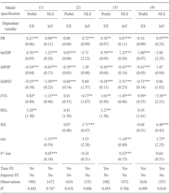
lnYit=α0+α1+PRDPit+α1−PRDNit+α2lnGDPit+α3lnPOPit+α4lnDISTi+α5FTAit+εit, (3) Different from the traditional gravity model, we further apply the HMR model to construct a two-stage estimation procedure to discern a firm’s binary decision to export into a given foreign market from their continuous decision of how much to export. As Briggs (2013) suggests, the probability that a firm would export is estimated by using a probit model in stage one for extensive margin of trade. The
number of exporters is controlled when estimating the volume of trade by using NLS in stage two for an intensive margin of trade.
In the first stage, the probability that the high-tech industry in Taiwan exports to country i can be characterized as follows:
EXit=β0+β1+PRDPit+β1−PRDNit+β2lnGDPit+β3lnPOPit+β4lnDISTi
+β5FTAit+β6RELit+νit
EXit= 1 if EXit*>0 , (4)
0 if EXit*=0
where EXit* is the export value of semiconductors from Taiwan to country i at year t, and RELi measures the similarity of religion in Taiwan and country i. We take the natural log of GDPit, POPit, DISTit, and RELi. All other variables in Eq. (4) are as explained for Eq. (3). Finally, νit is the normally distributed error term.
Studies dealing with selection models suggest that for the complete model to be identified, we should identify at least one factor that affects the decision variable but not the intensity variable (Lee and Park, 2016; Estrin et al., 2008; Maddala, 1983). As suggested by Helpman et al. (2008), Briggs (2013) and Lee and Park (2016), common religion is utilized as the instrument variable in the two-stage estimation procedure.2 Helpman et al. (2008) point out that common religion has a great influence on a firm’s choice of export, but not on its export volume once the exporting decision has been made.3 Helpman et al. (2008) and Briggs (2013) use data provided by La Porta et al. (1999), which capture the extent to which inhabit- ants in the two countries share a common religion on the religious composition of each country in our sample. In their study, common religion is computed as the following linear combination: REL=(% Protestants in country A * % Protestants in country B)+(% Catholics in country A * % Catholics in country B)+(% Muslims in country A * % Muslims in country B). Since Buddhism, Taoism and Christianity are the three major religions in Taiwan, we change the formula of common religion to: REL=(% Buddhists in Taiwan * % Buddhists in country i)+(% Taoists in Tai- wan * % Taoists in country i)+(% Christians in Taiwan * % Christians in country i) by using data provided by the CIA World Factbook.
In the second stage, the export volume in the semiconductor industry can be estimated as follows:
2 Briggs (2013) conducts an empirical study on high-tech exports as well, and thus we decided to use the common religion as the instrumental variable for the reason of comparison with Briggs (2013).
3 Helpman et al. (2008) also use the common language as the instrument variable, and obtain results almost identical to those using common religion.
lnYit=γ0+γ1+PRDPit+γ1−PRDNit+γ2lnGDPit+γ3lnPOPit+γ4lnDISTi
+γ5FTAit+ln{exp[δ(pˆi*+imˆrit*)]−1}+Bimrimˆrit*+ξit, (5) where Yit is the non-zero export value of the semiconductor industry’s goods from Taiwan to country i at year t, imˆrit* is the inverse Mills ratio estimated from the first stage probit equation used to correct for sample selection bias, and pˆi* is the predicted latent variable from the first stage estimation equation that captures the dichotomous export decision of firms. All other variables in Eq. (5) are explained for Eq. (3). Finally, ξit is the normally distributed error term. The sample selection of firms into certain exporting markets and the endogenous number of exporters of the stage one equation are isolated and controlled for stage two.
Under the specification of the difference in PRs protection, the stage one Probit estimation approximates the bilateral binary export decision. From this stage one equation, estimates of pˆi* and imˆrit* are derived and input non-linearly into the second stage equation of the volume of bilateral exports from the high-tech industry in Tai- wan to country i to correct for endogeneity and sample selection biases. The use of imˆrit* is the standard Heckman (1979) correction for sample selection. However, this does not correct for the biases generated by the underlying unobserved firm-level heterogeneity. The latter biases are corrected by the additional control pˆi*. The term, ln{exp[δ(pˆi*+imˆrit*)] −1}, controls for unobserved firm heterogeneity, that is, the effect of trade frictions and country characteristics on the proportion of exporters.
The standard Heckman correction is a valid estimation only in conditions where there is no firm-level heterogeneity, that is, where all firms are identically affected by trade costs. When firm-level heterogeneity is present and when there are fixed as well as variable trade costs, the consistent estimation method is a variant of the Heckman procedure that also corrects for the effect of exporting firms. The two-stage procedure of the HMR model is designed to correct for two potential problems in gravity equation estimations: selection bias resulting from dropping observations with zero trade volume, and bias due to unobserved firm-level heterogeneity resulting from a failure to measure the impact of exporting firms. In the second stage Eq. (5), two aspects of the first stage Eq. (4) are isolated and controlled for: (1) the sample selec- tion of firms into certain exporting markets and (2) the endogenous number of exporters. The interdependence of (1) and (2) results in the nonlinearity of the coefficient δ in Eq. (5), thus necessitating that Eq. (5) be estimated using non-linear least squares (NLS). The results then provide an unbiased estimate of the impact of the explanatory variables on the export volume of exporting firms.
According to Helpman et al. (2008), the two-stage estimation of the HMR model simultaneously corrects for the sample selection bias and the bias due to unob-
served firm heterogeneity embodied in the traditional gravity estimation of trade flows. The latter bias is due to an omitted variable that measures the influence of the number (fraction) of exporting firms (extensive margin). In a world without firm heterogeneity, or where such heterogeneity is not correlated with the export decision, all firms are indistinguishably affected by trade barriers and country characteristics and make the same export decision, or make export decisions that are uncorrelated with trade barriers and country characteristics. Then the potentially important effect of trade barriers and country characteristics on the share of exporting firms will be ignored. In a world with firm heterogeneity, firms are not equally affected by trade barriers and country characteristics, and make different export decisions. The esti- mation of the traditional gravity model confounds the effects of trade barriers and country characteristics on firm-level trade with their effects on the proportion of exporting firms. In Helpman et al. (2008), the empirical approach of the HMR model is driven from the theory they develop, and can be estimated with standard data sets. They argue that even without any firm-level data, it becomes possible to separately control for the number of exporting firms as well for the volume of trade per exporting firm corrected for the non-random export selection through the char- acteristics of the marginal exporters to different destinations. As a result, there exist sufficient statistics, which can be computed from aggregate data, to predict the selection of heterogeneous firms into export markets and their associated aggregate trade volumes. This is an important advantage of the HMR approach, which extracts from country-level data information that would normally require firm-level data.4
Santos Silva and Tenreyro (2015) suggest that the HMR probit model is incorrectly specified and casts doubts on any inference drawn from the empirical implementation of the HMR model. Instead, Santos Silva and Tenreyro (2006;
2010; 2011) propose an econometric solution to the “zero problem,” the PPML estimator. The Poisson model, used commonly for count data, can be applied more generally to non-integer variables and is equivalent to (weighted) non-linear least squares. The estimator is consistent under weak assumptions and the data need to be distributed as Poisson. Their point is in fact a very general one, whereby the econometric estimates of log-linearized models can be misleading because of the particular and noxious type of heteroscedasticity. The Poisson model enables the estimation of a gravity model, which includes the zeros. The dependent variable is trade, not log (trade). The independent variables still enter in logs and the coeffi-
4 For a more detailed description on the theoretical derivation, refer to Helpman et al. (2008), pages 449–457. Briggs (2013) further provides a theoretical discussion on how the HMR model is affected by the level of patent protection (Appendix A, pages 49–50).
cients can be interpreted as elasticities. For abstract reasons of statistical theory, Poisson is actually a very good workhorse estimator for gravity even if zeros are not a problem in the data. The type of heteroscedasticity that “the log of gravity”
deals with seems very common. Poisson implicitly assumes nothing “special”
about zeros, in which the problem is merely to consolidate the data into the esti- mation sample.
We finally conduct the PPML estimation on how the difference in PRs pro- tection between Taiwan and the trading countries affects Taiwan’s semiconductor exports. The empirical gravity equation of PPML model takes the following expo- nential function:
E(Yit|Zit)=exp(δ0+δ1+PRDPit+δ1−PRDNit+δ2lnGDPit+δ3lnPOPit+δ4lnDISTi
+δ5FTAit), (6)
where all variables in Eq. (6) are as they are explained for Eq. (3), and ξit is the nor- mally distributed error term. The vector Zit represents the explanatory variables.
The implementation of the PPML estimator is straightforward: there are standard econometric programs with commands that permit the estimation of Poisson regres- sion, even when the dependent variables are not integers. In particular, within Stata, the PPML estimation can be executed using a ready-to-use package directly. For a more detailed introduction of the estimation procedure of PPML, refer to Santos Silva and Tenreyro (2006).
For the robustness check, an importing country’s PRs protection level, PRit, is considered to examine the level impact of importing countries’ PRs protection rather than the difference in PRs protection. Since semiconductors are often regarded as intermediate goods and production inputs of other high-tech final goods (such as computers and smart phones), we also consider whether the industry structure, rep- resented by the ratio of high-tech exports to manufacturing exports of the importing country, HXit, will influence Taiwan’s semiconductor exports. We compare the results of Eqs. (3), (4), (5) and (6) under these specifications.
IV. Data
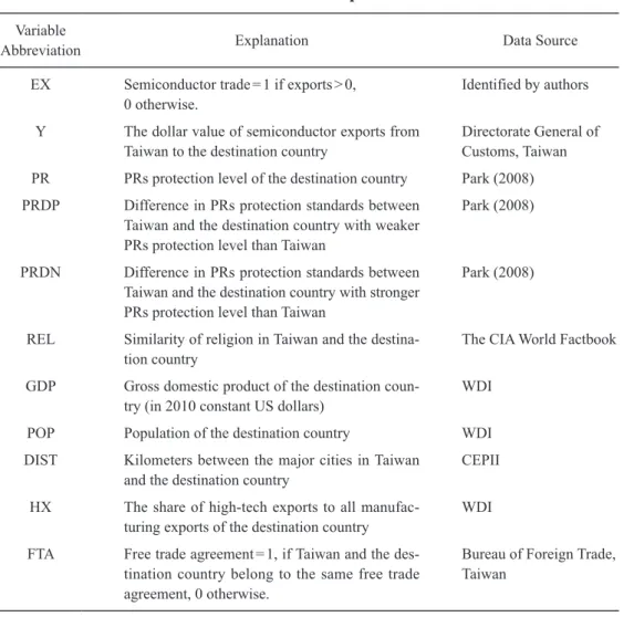
Table 1 explains the data used in this paper and their sources. Table 2 provides a statistical summary of the variables. Park (2008) updates the Ginarte-Park Index, ranging from 0 (no protection) to 5 (strongest protection), for 122 selected countries for the period of 1960–2005 at five-year intervals.5 After excluding Taiwan (as the
5 For the period of 2006–2010, we assume the indices are identical to that of 2005. For the period of
Table 1: Variable Explanations
Variable
Abbreviation Explanation Data Source
EX Semiconductor trade=1 if exports>0,
0 otherwise. Identified by authors
Y The dollar value of semiconductor exports from
Taiwan to the destination country Directorate General of Customs, Taiwan PR PRs protection level of the destination country Park (2008) PRDP Difference in PRs protection standards between
Taiwan and the destination country with weaker PRs protection level than Taiwan
Park (2008)
PRDN Difference in PRs protection standards between Taiwan and the destination country with stronger PRs protection level than Taiwan
Park (2008)
REL Similarity of religion in Taiwan and the destina-
tion country The CIA World Factbook
GDP Gross domestic product of the destination coun-
try (in 2010 constant US dollars) WDI
POP Population of the destination country WDI
DIST Kilometers between the major cities in Taiwan
and the destination country CEPII
HX The share of high-tech exports to all manufac-
turing exports of the destination country WDI FTA Free trade agreement=1, if Taiwan and the des-
tination country belong to the same free trade agreement, 0 otherwise.
Bureau of Foreign Trade, Taiwan
exporting country in this study) and two other nations (Somalia and Syria) for which the World Development Indicator (WDI) database does not provide the data of both GDP and population; the remaining 119 countries are chosen as the importing (des- tination) countries in this study. Therefore, the full sample size of our study is 1,904
1995–2005, we employ three measures to construct the indices for various years. First, we assume PRs improves gradually over time, so we calculate the average annual growth rate of indices between 1995 and 2000 and then obtain the index for 1996 by multiplying that of 1995 by the average annual growth rate. Second, we assume the indices for 1996 and 1997 are the same as that of 1995 and the indices for 1998 and 1999 are the same as that of 2000. Third, we assume the indi- ces for 1995–1999 are identical to that of 1995. We find that the estimates are similar for different measures, and the results reported in the empirical analyses adopt the third measure.
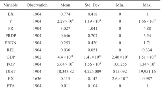
Table 2: Summary Statistics
Variable Observation Mean Std. Dev. Min. Max.
EX 1904 0.774 0.418 0 1
Y 1904 2.29×10⁸ 1.19×10⁸ 0 1.66×10¹⁰
PR 1904 3.027 1.041 0 4.88
PRDP 1904 0.646 0.707 0 3.54
PRDN 1904 0.253 0.420 0 1.71
REL 1904 0.036 0.051 0 0.334
GDP 1902 4.4×10¹¹ 1.41×10¹² 2.40×10⁸ 1.51×10¹³
POP 1904 5.04×10⁷ 1.56×10⁸ 100,255 1.34×10⁹
DIST 1904 10,343.82 4,225.009 815.092 19,951.16
HX 1636 0.115 0.142 2.6×10⁻⁶ 0.987
FTA 1904 0.011 0.104 0 1
(119 countries times 16 years). We downloaded export data from the online database of Taiwan’s Directorate General of Customs. Among 1,904 observations, around 22.6% of the sample (430 observations) has zero export value (Y), i.e. EX=0. The average of the Ginarte-Park Index for our sample countries during 1995–2010 is 3.027, and the average of semiconductor exports is US$229 million. As a natural logarithm of 0 is undefined, we usually run the log-linearized gravity model for observations with positive trade value only. However, dropping zeros means we are getting rid of potentially useful information. We might be able to learn why certain countries trade in products, while others do not. By using only a portion of the available data, we might be producing biased estimates of the coefficients we are primarily interested in. Recent literature has paid considerable attention to the “zero trade problem.” Three main approaches to overcome the problem are the (1) ad hoc solution, (2) HMR model, and (3) PPML. The ad hoc solution means adding a small, positive number (e.g., 1 in our study here) to all trade flows and seeing if including or excluding zeros appears to make a difference empirically. This approach is com- monly used in policy literature, but has no theoretical basis, and is approximate at best (De, 2013). In the following sub-sections, we explain the three approaches in detail accordingly.
The religious population data provided by the CIA World Factbook is used to calculate common religion (REL), which ranges from 0 to 0.334. GDP, population (POP) and high-tech export share (HX) are collected from WDI, and the geographic distances between the major cities in Taiwan and the destination country are obtained
from CEPII. The maximum value of HX is 0.987 (Singapore, 2006), while the mini- mum value is 0.0000026 (Nepal, 1999). After checking the website of Taiwan’s Bureau of Foreign Trade, we identify five countries which had signed FTAs with Taiwan during 1995–2010: Panama (June, 2002), Guatemala (July, 2006), Nicara- gua (January, 2008), El Salvador (March, 2008) and Honduras (July, 2008). The detailed figures of common religion and the trends of the Ginarte-Park index (PR) and export value (Y) for 119 destination countries are provided in the Appendix.
In Table 2, two variables are found to have missing values. GDP has two miss- ing values because there is no GDP data for Haiti and Iceland in 1995. In contrast, HX suffers a more serious missing data problem and has 268 missing values.
Therefore, in order to keep more observations in our regressions, HX is used for the robustness check only. The maximum number of observations which can be used in the regressions is 1,902.
V. Empirical Results
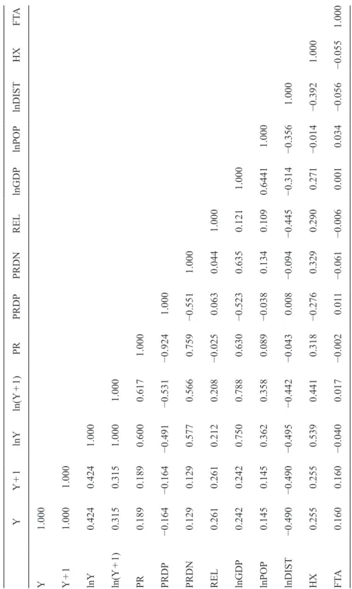
1. Specification TestsTable 3 provides the pairwise correlation matrix of variables used in our study.
Two observations are worth noting. First, a correlation value of 1 between lnY and ln(Y+1) (which is the ad hoc solution of the zero trade), as well as between Y and Y+1, implies that the two pairs of variables are almost the same. Second, the pair correlation of PRs protection (PR) and PRDP is about −0.924 and that of PR and PRDN is around 0.759, which exceed the minimum threshold of strong correlation, 0.7.
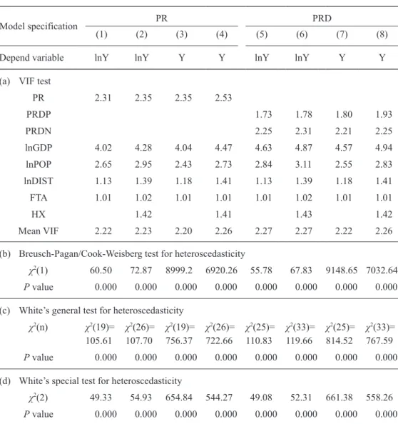
To check further for a multicollinearity problem among these variables, we conduct variance inflation factor (VIF) tests, which are reported in Part (a) of Table 4. The square root of the VIF value indicates how much larger the standard error is, compared with the value if that variable is uncorrelated with the other predictor variables in the model. Columns (1) to (4) and Columns (5) to (8) of Table 4 are the test results based on different model specifications with PR and PRD and different dependent variables (lnY and Y), respectively. A VIF value of 1 means there is no correlation among the kth predictor and the remaining predictor variables. Hence, the variance of bk is not inflated. The general rule of thumb is that VIF values exceeding 5 warrant further investigation, whereas VIF values exceeding 10 are signs of serious multicollinearity requiring correction. All model specifications, no matter which the dependent variable is, have VIF values less than 3, which in turn guarantees that there is no multicollinearity problem.
Estimations of OLS and HMR are based on the assumptions of normality and
Table 3: Pairwise Correlation Matrix YY+1lnYln(Y+1)PRPRDPPRDNRELlnGDPlnPOPlnDISTHXFTA Y1.000 Y+11.0001.000 lnY0.4240.4241.000 ln(Y+1)0.3150.3151.0001.000 PR0.1890.1890.6000.6171.000 PRDP−0.164−0.164−0.491−0.531−0.9241.000 PRDN0.1290.1290.5770.5660.759−0.5511.000 REL0.2610.2610.2120.208−0.0250.0630.0441.000 lnGDP0.2420.2420.7500.7880.630−0.5230.6350.1211.000 lnPOP0.1450.1450.3620.3580.089−0.0380.1340.1090.64411.000 lnDIST−0.490−0.490−0.495−0.442−0.0430.008−0.094−0.445−0.314−0.3561.000 HX0.2550.2550.5390.4410.318−0.2760.3290.2900.271−0.014−0.3921.000 FTA0.1600.160−0.0400.017−0.0020.011−0.061−0.0060.0010.034−0.056−0.0551.000
Table 4: VIF and Heteroscedasticity Tests
Model specification PR PRD
(1) (2) (3) (4) (5) (6) (7) (8)
Depend variable lnY lnY Y Y lnY lnY Y Y
(a) VIF test
PR 2.31 2.35 2.35 2.53
PRDP 1.73 1.78 1.80 1.93
PRDN 2.25 2.31 2.21 2.25
lnGDP 4.02 4.28 4.04 4.47 4.63 4.87 4.57 4.94
lnPOP 2.65 2.95 2.43 2.73 2.84 3.11 2.55 2.83
lnDIST 1.13 1.39 1.18 1.41 1.13 1.39 1.18 1.41
FTA 1.01 1.02 1.01 1.01 1.01 1.02 1.01 1.01
HX 1.42 1.41 1.43 1.42
Mean VIF 2.22 2.23 2.20 2.26 2.27 2.27 2.22 2.26
(b) Breusch-Pagan/Cook-Weisberg test for heteroscedasticity
χ2(1) 60.50 72.87 8999.2 6920.26 55.78 67.83 9148.65 7032.64 P value 0.000 0.000 0.000 0.000 0.000 0.000 0.000 0.000 (c) White’s general test for heteroscedasticity
χ2(n) χ2(19)=
105.61
χ2(26)=
107.70
χ2(19)=
756.37
χ2(26)=
722.66
χ2(25)=
110.83
χ2(33)=
119.66
χ2(25)=
814.52
χ2(33)=
767.59 P value 0.000 0.000 0.000 0.000 0.000 0.000 0.000 0.000 (d) White’s special test for heteroscedasticity
χ2(2) 49.33 54.93 654.84 544.27 49.08 52.31 661.38 558.26 P value 0.000 0.000 0.000 0.000 0.000 0.000 0.000 0.000
homoscedasticity. The estimations may be inconsistent if the data exhibits heterosce- dasticity, which is usually found in panel data such as that used in this study. Three tests for heteroscedasticity, the Breusch-Pagan/Cook-Weisberg test, White’s general test and White’s specific test, are conducted and their results are reported in Parts (b) to (d) of Table 4. All tests confirm the existence of heteroscedasticity. Therefore, PPML should be used to obtain consistent estimations. In the next subsection, we will report the estimation results of PPML, followed by those of OLS and HMR for comparisons.
2. Results from PPML
Tables 5 and 6 show the results estimated by PPML. Columns (1) to (5) of Table 5 exhibit different model specifications of time and importer fixed-effects on estimating the impact of PRs differences (PRD) on the semiconductor exports.
Column (2) is applied for observations with the positive export value (i.e., Y > 0).
In addition, Column (6) is a robustness check, adding an extra variable, high-tech export share (HX). Overall, country size and distance have expected signs in the gravity model, i.e. a positive coefficient for GDP (lnGDP) and a negative one for distance (lnDIST). Population (lnPOP) has a negative impact on the semiconductor exports, which might reflect the fact that only small amounts of semiconductors are shipped to less developed countries with large populations which do not have
Table 5: PPML Estimation of the Impact of the Differences in PRs Protection
Model specification (1) (2) (3) (4) (5) (6)
Dependent variable Y Y>0 Y Y Y Y
PRDP −2.45***
(0.41)
−2.43***
(0.41)
−1.68***
(0.29)
−1.83***
(0.38)
−0.89***
(0.31)
−0.90***
(0.31)
PRDN −1.06***
(0.19)
−1.05***
(0.19)
−0.60***
(0.17)
0.05 (0.19)
1.31***
(0.39)
1.31***
(0.39)
lnGDP 0.94***
(0.06)
0.94***
(0.06)
0.83***
(0.05)
2.51***
(0.33)
0.88***
(0.24)
0.84***
(0.25)
lnPOP −0.38***
(0.06)
−0.38***
(0.06)
−0.35***
(0.05)
−0.71 (0.78)
−2.32***
(0.76)
−2.21***
(0.80)
lnDIST −1.70***
(0.06)
−1.69***
(0.06)
−1.75***
(0.05)
−2.00***
(0.47)
−3.32***
(0.38)
0.60 (0.97)
FTA 0.20
(0.15)
0.20 (0.15)
0.01 (0.21)
−0.07 (0.07)
−0.07 (0.06)
−0.08 (0.06)
HX 0.16
(0.30)
Time FE No No Yes No Yes Yes
Importer FE No No No Yes Yes Yes
Observations 1902 1472 1902 1838 1838 1589
R2 0.788 0.785 0.820 0.953 0.979 0.979
Notes: Robust standard errors are reported in parentheses.
*** Significant at 1 percent level. ** Significant at 5 percent level. * Significant at 10 percent level.
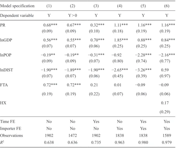
Table 6: Robustness Check for PPML Estimation
Model specification (1) (2) (3) (4) (5) (6)
Dependent variable Y Y>0 Y Y Y Y
PR 0.68***
(0.09)
0.67***
(0.09)
0.32***
(0.10)
1.11***
(0.18)
1.16***
(0.19)
1.16***
(0.19)
lnGDP 0.56***
(0.07)
0.55***
(0.07)
0.70***
(0.06)
1.85***
(0.25)
0.88***
(0.25)
0.84***
(0.25)
lnPOP −0.19**
(0.09)
−0.19**
(0.09)
−0.31***
(0.07)
−0.92 (0.80)
−2.28***
(0.74)
−2.16***
(0.77)
lnDIST −1.90***
(0.07)
−1.89***
(0.07)
−1.90***
(0.06)
−2.65***
(0.45)
−3.26***
(0.39)
0.59 (0.97)
FTA 0.72*** 0.72*** 0.21 0.01 −0.09 −0.09
(0.19) (0.19) (0.22) (0.07) (0.06) (0.06)
HX 0.17
(0.29)
Time FE No No Yes No Yes Yes
Importer FE No No No Yes Yes Yes
Observations 1902 1472 1902 1838 1838 1589
R2 0.638 0.636 0.735 0.963 0.980 0.979
Notes: Robust standard errors are reported in parentheses.
*** Significant at 1 percent level. ** Significant at 5 percent level. * Significant at 10 percent level.
the technological capability to turn semiconductors, the intermediate goods, into high-tech final goods, such as computers and smart phones. The impact of free trade agreements (FTA) is insignificant, which is not surprising at all given that few FTAs were signed during the sample period.
The results in Columns (1) (with 1,902 observations) and (2) (with 1,472 obser- vations), in which we do not control for either the time fixed-effect or the importer fixed-effect, are indistinguishable quantitatively, and the value of R-squared is around 0.79. Similarity is found between Columns (1) (with 1,902 observations) and (2) (with 1,472 observations) of Table 6 when we explore the impact of PRs (PR). Fur- thermore, the results in Columns (3) and (4) of Table 5, which control for the time fixed-effect and the importer fixed-effect, respectively, still support a negative and statistically significant coefficient for PRDP, but the coefficient of PRDN becomes positive (0.05) and insignificant in Column (4). Their values of R-squared improve
to 0.82 and 0.95, respectively. Column (5), in which we control both time and importer fixed effects, has the highest value of R-squared (0.979) among Columns (1) to (5) and shows a positive and statistically significant coefficient for PRDN.
Along with the finding of a negative and significant coefficient for PRDP, it implies that improvements in international patent regimes do encourage Taiwan’s semicon- ductor exports.
To test whether the results obtained from PPML are consistent, we add HX in Column (6) under the specification similar to Column (5). This modification reduces the number of observations from 1,838 to 1,589 due to the missing values in HX, but the results are quite similar, except that the impact of distance on the semiconductor exports now becomes positive and insignificant. All specifications in Table 6 sup- port a positive impact of PRs protection on the semiconductor exports. Therefore, we may conclude that the impacts of both PRD and PR are robust under different model setups.6
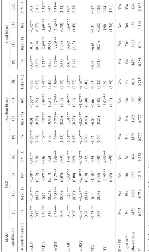
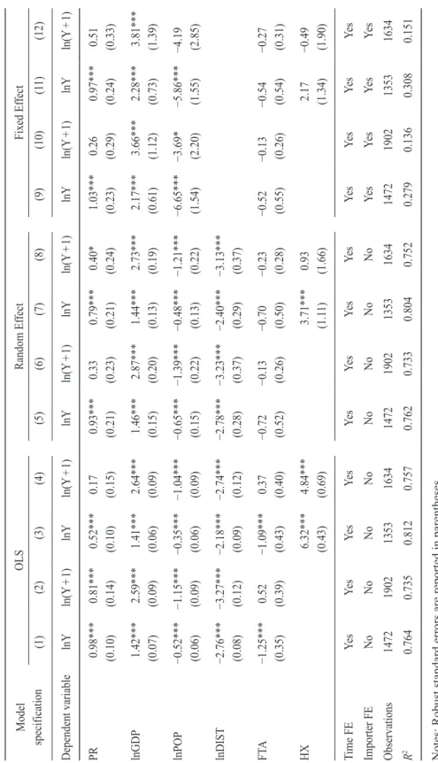
3. Results from Traditional Gravity Model
Table 7 provides the results of the impact of PR differences (PRD) on Taiwan’s semiconductor exports for OLS, random effect and fixed effect models. Columns (1) to (4) of Table 7 illustrate four model specifications for OLS estimations on the impact of PRD. These specifications are (1) the basic model for the positive export observations only, (2) the basic model with the ad hoc solution, (3) the model includ- ing HX for the positive export observations only, and (4) the model including HX with the ad hoc solution. Several findings are worth noting. First, with 430 obser- vations with zero export value, the results in Column (1) are dissimilar to the val- ues in Column (2), i.e., adding a positive and small number, which is 1 here, into export value does alter the results qualitatively. Second, PRDP (PRDN) has signifi- cant and negative (positive) impact on Taiwan’s semiconductor exports and export elasticity ranging from −0.30 to −0.85 (0.97 to 1.31) based on different specifica- tions in Columns (1) and (3). The impact of PRDN becomes insignificant in Col- umns (2) and (4) when the ad hoc solution is applied. Third, adding an extra vari- able (HX) changes the coefficients of PRDP and PRDN substantially when the
6 As also observed later in the estimations of traditional gravity model and HMR, in all regressions with the importer fixed-effect, the coefficient on HX is never significant. Moreover, in the HMR estimations, including HX will cause the first stage coefficients on REL to become insignificant, suggesting that there may be some multicollinearity problems. Therefore, our discussions hereafter will focus on the results from regressions without HX.