建置民用航空全球衛星定位系統陸基增強系統測試平台之研究發展與評估

全文

(1)行政院國家科學委員會專題研究計畫成果報告建置民用航空全球衛星定位系統陸基增強系統測試平台之研究發展與評估研究成果報告(精簡版). 計計執執. 畫畫行行. 類編期單. 別號間位. ：個別型： NSC 98-2221-E-006-122： 98 年 08 月 01 日至 99 年 07 月 31 日：國立成功大學航空太空工程學系（所）. 計畫主持人：詹劭勳計畫參與人員：碩士級-專任助理人員：林耀正碩士班研究生-兼任助理人員：蔡文明碩士班研究生-兼任助理人員：陶安麟碩士班研究生-兼任助理人員：張凱荏. 報告附件：出席國際會議研究心得報告及發表論文. 處理方式：本計畫可公開查詢. 中. 華. 民. 國 99 年 10 月 07 日.

(2) 目錄 1. 前言 ................................1 2. 研究目的 ............................1 3. 文獻探討 ............................2 4. 研究方法 ............................3 4.1. . 修正量與載波平滑法.............................................................................................. 3 . 4.2. . 品質監控.................................................................................................................. 4 . 4.3. . Common Set ........................................................................................................... 7 . 4.4. . 一致性驗證.............................................................................................................. 7 . 4.5. . EXM ........................................................................................................................ 9 . 4.6. . σμ monitor .............................................................................................................. 9 . 4.7. . 修正量範圍測試.................................................................................................... 10 . 5. 結果與討論 .........................11 6. 本專題計畫相關論文發表 .............12 7. 參考文獻 ...........................13 8. 圖表 ...............................14 .

(3) 1. 前言陸基增強系統(Ground Based Augmentation System, GBAS)是一套輔助全球導航衛星系統(Global Navigation Satellite System, GNSS)的增強系統，加強在區域性範圍內可以提供較 GNSS 完整性(Integrity)更高的定位能力，使該系統的導航性能足以提供給飛航上作精確進場(Precision Approach, PA)的使用。以取代現有的儀器降落系統(Instrument Landing System, ILS)作為民航上使用的主要導航系統。目前全球發展的 GNSS，以美國所發展與運行的全球定位系統(Global Positioning System, GPS)最為完整，故本專題研究將開發陸基增強系統原型機 (GBAS prototype)進行 GBAS 在台灣飛航情報區之效能測試評估，透過執行本專題計畫，其評估分析結果將提供國家在未來先進航管(CNS/ATM)系統建置 GBAS 相關系統的重要參考。本專題計畫原訂兩年期計畫執行完成，但國科會只核定第一年計畫，因此本計畫報告將以原計畫書所提之第一年研究發展工作項目提出成果報告。. 2. 研究目的在民用航空領域中，已經有許多已開發的導航接收器利用 GPS 進行定位，例如一般民用航空客機利用 GPS 接收器於飛越海洋或者是橫跨大陸航線之導航。隨著 GPS 導航技術的進步與成熟，運用 GPS 進行民用航空客機的進場 (approach)與自動降落(landing)已經成為一種趨勢；然而民用航空客機對於進場與自動降落系統的系統穩定度以及安全性是非常重視的，單靠全球導航衛星系統本身並不足夠滿足全部的民用導航需求[1]。為了解決這個問題，我們必須要依靠增強系統(augmentation system)來加強 GPS 的效能，其中，陸基增強系統(Ground Based Augmentation System, GBAS)是一套建構在機場的區域性系統，其有鑑於對進場階段的需求，在特定範圍內提供服務，輔助衛星導航系統並滿足民用航空客機對精確進場在精確度(accuracy)、完整性(integrity)、可用性(availability)、連續性(continuity) [1]上的要求，如圖一與表一，正是一個很好的解決方案。以現階段而言，GPS 在精確度方面的表現對於一般民用導航已經足夠，最欠缺的部份反而是完整性(integrity)方面的監測，且此部分會連帶影響到可用性與連續性，這也就成為陸基增強系統最主要的目標。完整性的意義在於及時地提供使用者關於系統是否可以使用該系統的警告，如圖一，最左邊的圖是單獨使用 GPS 定位的情形，其中圓心為真實位置、其餘的點為 GPS 定位解、實線的圓圈表示在民航上可以容忍的最大定位誤差、虛線的圓圈表示 95%的定位誤差，由圖中可以發現此時 95%的定位誤差大於民航上可以容忍的最大定位誤差，使用者可以很明確地知道單只使用 GPS 在精確度上無法滿足民航的導航要求；然而，透過差 1 .

(4) 分定位(Differential GPS, DGPS)的技術便能輕易地降低 GPS 定位解的誤差，如同圖一右邊所示，位置解更集中於真實位置，但仍有一些誤差較大的定位解落在實線圓圈之外，此種危險的情形在民航上稱為 Hazardous Misleading Information (HMI)，也就是使用者以為 GPS 可以使用，但實際上卻有可能發生過大的定位誤差；圖一中間則為使用陸基增強系統之後的情形，此時的定位解誤差比差分定位來的大，是因為其提供的完整性資訊會刪除掉可能造成過大定位誤差衛星，但卻能夠保證使用者的安全（沒有任何一定位解落於時線圓圈外），這也是陸基增強系統最主要的目的。本年度專題計畫將利用 GPS 之衛星訊號，進行研究、發展與建置可應用於特定區域(specific local area)之陸基增強系統原型機(GBAS prototype)，其中包含天線架設與站台安裝等硬體建置以及主站演算法的軟體設計。. 3. 文獻探討陸基增強系統除了能提供精確進場導航外，還能提供飛機離場時的導引，相較於 ILS，陸基增強系統之效能更為強大且不受天候影響，因此，目前有許多國家皆投入發展，除了發展最早美國的區域增強系統（Local Area Augmentation System, LAAS）外，巴西、日本、韓國、德國等國家皆在建立陸基增強系統。其中日本與德國已在飛測階段，巴西與韓國屬於初期開發階段。 LAAS 是經由美國聯邦航空總署認可後部署，主要是針對機場設置。此一增強的計畫，是為了期望能將衛星導航裝備由輔助系統提升為主要裝備，以適合民航使用。LAAS 主要可分成地面設備以及航空電子設備，其中包括計算和傳送修正與完整性資料（Corrections and Integrity Messages）給使用者。地面設備包含四個參考 GPS 接收器、LAAS 地面設施(LAAS Ground Facility, LGF)和 VHF 資料廣播發送台（VHF Data Broadcast, VDB）。接收器與地面設施分工，計算出 GPS 位置解的誤差及相關誤差範圍，再使用 108 到 118MHz 的頻段，由 VDB 播送給 LAAS 涵蓋範圍（約 20-30 哩）內的使用者。如要進一步加強在垂直方向上的表現，LAAS 可額外增加虛擬衛星（Pseudolite）的設置，虛擬衛星傳送與 GPS 相同的訊號，使用者在定位時相當於有一顆衛星在下方，使衛星的幾何分佈變好，進而增進垂直高度。在美國聯邦航空局(Federal Aviation Administration, FAA)方面，在 2009 年 LAAS 完成認證成為新一代的 CAT I 降落系統，2010 年起進行 LAAS 在 CAT II/III 的可行性與風險評估。LAAS 的精確度與完整性確實滿足 CAT I 的要求，在自動降落時提供機場導航資訊給飛行載具，落地之後，更可以利用 LAAS 帶領飛行載具引導至登機門。在前述的國家中，只有巴西位於低緯度地區。由於巴西地區的電離層活動極為劇烈，目前巴西研究測試的目標是為了確保在受電離影響劇烈的巴西，是否能有效通過檢測順利發展陸基增強系統。 2 .

(5) 4. 研究方法首先，在硬體架構上包含三個參考站跟一個主站，其中各參考站儲存來自 GPS 衛星的資料，每個參考站包含一個使用者工作平台、一個雙頻接收機、一個天線盤與一組腳架和球心基座，天線盤會透過同軸電纜，傳送接收到的 GPS 衛星訊號至雙頻接收機，接著雙頻接收機會將 GPS 衛星訊號進行解碼，並包裝成特定格式，之後便可以透過使用者工作平台與 RS-232 通訊協定，從雙頻接收機取得陸基增強系統原型機演算法所需的資料並儲存，接下來便由主站整合所有參考站資料，進行陸基增強系統原型機演算法產生修正量與完整性訊息，最後產生評估結果，如圖二。陸基增強系統原型機演算法流程如圖三所示，首先各參考站透過接收器儲存 GPS 衛星資料，其中包含長效型星曆(almanac)、短效型星曆(ephemeris)與 GPS 雙頻觀測量，此資料將被送至陸基增強系統原型機伺服器並且開始針對各參考站的觀測量進行品質監控，其中包含：觀測量品質監控(Measurement Quality Monitoring, MQM)、訊號品質監控(Signal Quality Monitoring, SQM)與資料品質監控(Data Quality Monitoring, DQM)，而這三個品質監控 (Monitoring)會各自進行兩個或三個監測(Tests)來滿足品質上的監控目的。上述三個品質監控系統皆會個別針對每一個接收到的衛星訊號產生標記 (Flag)來表示該衛星是否通過該品質監控系統，三個參考站各有獨立的三個品質監控系統，所以需要一個強健的判斷流程也就是 Executive Monitoring (EXM)機制，用以決定有哪些衛星在後續的計算中必須被排除。接下來將會針對剩餘的衛星進行載波平滑法(Carrier smooth)來降低參考站收到的觀測量雜訊，並且得到量測距離之修正量(Pseudorange Correction, PRC)與其誤差信心範圍(Error confidence bound)，也就是使用者所需要的修正量與完整性訊息，其中修正量又可分為電碼(code)與載波(carrier phase)修正量。然而在傳送修正量與完整性訊息給使用者之前，主站還會進行後續的檢測，其中包含一致性驗證(Multiple Reference Consistency Check, MRCC)、平均修正量之變異數的監控(Sigma mean monitor, σμ monitor)與修正量範圍測試(Message Field Range Test, MFRT)，確保使用者的安全，維持系統的完整性需求。. 4.1. 修正量與載波平滑法主站首先會利用載波平滑法(Carrier smooth)來降低參考站收到的觀測量雜訊，而載波平滑法之演算法如下[2]:. 3 .

(6) ρ s ,m,n (k ) =. 1 W −1 ⎡ ρ s ,m,n (k − 1) + φm ,n (k ) − φm ,n (k − 1) ⎤⎦ ρ m,n (k ) + W W ⎣. (1). 其中. W=. τd Ts. =. 100 = 200 12. (2). ρn 及 φn Φ 分別為 n 號衛星的電碼波與載波之觀測虛擬距離； τ d 為載波平滑法用來控制收斂區間的時間常數，在此為 100 秒[3]；Ts 為接收觀測量之頻率，在此為 0.5 秒；底標(m,n)為參考站 m 與衛星 n 的配對。經由載波平滑法後，我們可使部分誤差之影響性降低，接著再利用此衛星觀測量與相關文獻中所規範之演算法產生各個衛星的修正量。由於各個參考站之精確位置是已知的，因此可以利用衛星所發佈的星曆資料來計算衛星位置與各個參考站之間的真實距離來與前面經過載波平滑法運算後的量測距離進行計算，進而得到量測距離之修正量，計算量測距離之修正量方式如下[3]. ρ sc ,m,n (k ) = ρ s ,m,n (k ) − Rm,n (k ) − τ m,n (k ). (3). φc ,m,n (k ) = φm,n (k ) − Rm,n (k ) − τ m,n (k ) − φci ,m,n . (4). 其中. φci ,m,n = φm,n (0) − Rm,n (0) − τ m,n (0) . (5). φci ,n 為載波修正量初始值，甫接收到衛星訊時時便會計算並儲存，目的是用來消除載波修正量的整數週波未定值(integer ambiguity)，每當發生週波脫離(cycle slip) 時便會重新計算。. 4.2. 品質監控每個參考站收到的衛星資料都必須執行品質監控，避免誤差過大的衛星影響到路基增強系統的完整性，其包括 SQM、DQM 與 MQM，每個 QM 中各有二到三個測試，如圖四，而用來產生陸基增強系統服務訊息的衛星必須要通過所有的 4 .

(7) 測試。每個參考站的每個測試都有專屬的測試值(test statistic)與門檻值 (threshold)，測試值將會與門檻值互相比較當作衛星是否通過測試的依據；如果測試值超過門檻值，該衛星便會被判定為沒有通過品質監控。每個參考站的每個測試的門檻值都是透過 Gaussian Overbounding Method (GOM)[4][5][6]計算得到，這個方法是利用長時間收集的資料，透過統計的方式，依據不同的衛星仰角找出適用的門檻值。. A、訊號品質監控：此監控的目的在於確認 GPS 訊號本身的品質，一般來說品質越差的訊號較容易產生誤差，此監控包含訊號強度測試(signal power test) 與相異測試(divergence test)。訊號強度測試是利用衛星的載波強度與雜訊強度比(C/N0)做為測試值，計算方式如下[7] C N 0,avg ,m ,n (k ) =. 1 ⎡C N 0,m,n ( k − 1) + C N 0,m ,n ( k ) ⎦⎤ 2⎣. (6). 由於 C/N0 越低就代表訊號強度越低，所以通過訊號強度測試的條件就是，此測試值是必須高於門檻值，藉此排除掉 C/N0 過低的衛星。相異測試的目的是檢查 GPS 的電碼與載波觀測量差異，測試值計算方法如下[2]. Dvgcm,n (k ) =. τ d − Ts 1 Dvgcm,n (k − 1) + dzm,n (k ) τd τd. (7). 其中. zm,n (k ) = ρ m ,n (k ) − φm,n (k ) . (8). dzm ,n (k ) = zm ,n (k ) − zm ,n (k − 1) . (9). 藉由檢視這個差異可以防止差分修正量發生錯誤。如此之外，這個差異主要是由電離層所引起，若是差異過大，表示此時的 GPS 的觀測量受到電離層的影響過大不適合使用，這個差異值同樣也會與一門檻值做比較，做為是否要排除的依據。 B、資料品質監控：此監控的目的在於驗證 GPS 接收器取得的星曆是否正確，而星曆又可分為長效型(almanac)與短效型(ephemeris)，陸基增強系統以短效型星曆為主，透過較為精確的衛星位置來提供更準確的修正量，因此星曆錯誤會直接造成修正量上發生錯誤，資料品質監控的責任就是排除掉此種情形。雖然星曆會持續地更新，但新舊星曆計算出來的衛星位置在正常 5 .

(8) 的情況下不會差距太多，於是這個部分就依此比較新舊星曆之間的差距，做為是否要排除的依據。除此之外，資料品質監控也會比較長效型與短效型星曆計算出來的衛星位置，若是同一顆衛星的差距過大，也會進行排除的動作。在資料品質監控比較衛星位置時，會由收到短效型星曆的時間點，每隔五分鐘計算出未來六個小時的衛星位置做為測試值，其中新舊星曆計算出來的衛星位置差要低於 250 公尺；長效型與短效型星曆計算出來的衛星位置差要低於 7000 公尺[8][9]。 C、觀測量品質監控：此監控的目的是用來檢視觀測量是否有不正常的變化，其中包括鎖定時間確認(lock time check)、載波測試(acceleration-ramp-step test)和電碼測試(innovation test)。首先，鎖定時間確認會針對每顆衛星判斷其訊號是否有持續地被接收到，做為部分演算法重新執行的依據，但並不會做任何排除的處理；因為即使是發生周波脫落，但由於一個波的長度很小，並不足以影響到使用者的安全性。載波測試則是用來檢驗載波觀測量是否有不正常跳動的情形，如果跳動過大表示受到誤差源的影響過大，必須排除以確保修正量所提供的準確度與完整性。做法是透過蒐集連續十筆的觀測量，並在每一秒算出每顆衛星的載波修正量與所有衛星修正量之間的差值如下. φm* ,n (k ) = φc ,m ,n (k ) −. 1 N. ∑. j∈Sm ( k ). φc ,m, j (k ) . (10). 其中 S m 為第 m 個參考站收到的十筆連續觀測量都有存在的衛星組合，N 則是此衛星組合內的衛星數量。接下來採用最小平方法，依照以下二項式估算這十筆差值的趨勢[2]. φ. * m ,n. d 2φm* , n (k , t ) t 2 dφm* , n (k , t ) (k , t ) = ⋅ + ⋅ t + φm* ,n (k ) 2 dt 2 dt. (11). 載波測試的測試值便是此二項式的係數，分別是. Accm ,n (k ) ≡. d 2φm* ,n (k , t ). Rampm ,n (k ) ≡. dt 2. dφm* ,n (k , t ) dt. (12). . (13). . 除此之外，載波測試還會利用此二項式估算出來的趨勢預測第十一秒的差值，用來與第十一秒的實際值相減，此差值便是載波測試的第三個測試值，定義為 6 .

(9) Stepn (k ) ≡ φn* (k ) − φn* (k − 1, 10 ⋅ Ts ) . (14). 這三個測試值都會與個別的門檻值互相比較，做為排除衛星的依據。除了載波觀測量之外，觀測量品質監控還會對電碼觀測量進行監測，這個電碼測試利用載波變異量較小的特性，應用其差值來預測下一秒的電碼觀測量，測試值計算方式如下[2]. Innon (k ) ≡ ρ n (k ) − ⎡⎣ ρ s ,n (k − 1) + φn (k ) − φn (k − 1) ⎤⎦ . (15). 這個測試值同樣地也會與其專屬的門檻值互相比較，藉此排除掉觀測量跳動過大的衛星。. 4.3. Common Set Common Set 為 EXM 的一部分，主要負責邏輯上的判斷，由於三個參考站各有三個不同的品質監控系統，會個別針對每一個所接收到之衛星訊號產生標記 (Flag)來表示該衛星是否通過該品質監控系統，所以在第一階段的工作就是判斷並排除被標記的衛星；圖五為如何排除衛星所舉的例子，圖中的橫軸表示衛星號碼；縱軸表示參考站編號；T 表示該衛星的訊號被所對應的參考站接收，並且通過三個品質監控；F 表示該衛星的訊號被所對應的參考站接收，但至少有一個品質監控沒有通過；N 表示該衛星的訊號並沒有被所對應的參考站接收到，也不會進行任何一項品質監控的測試。主站的服務訊息將由三個參考站所共同接收且通過三個品質監控系統的衛星來產生，而此衛星組合便稱為 Common Set [3][10]。在圖五中，雖然虛線內的衛星數目較多，但此時主站會採用實線內的衛星組合做為 Common Set；除非 Common Set 的衛星數小於四個，主站便會採用虛線的方式，改由兩個參考站進行上述程序找出 Common Set 來產生服務訊息，以避免衛星數過少影響結果；如果還是沒有辦法找出大於四顆，則此時無法提供服務。. 4.4. 一致性驗證產生修正量之後，便會進入一致性驗證的流程。由於環境相似的關係，正常的情形之下各衛星的修正量差異不大，所以這個階段的目的主要是透過三個參考站交互確認修正量是否有發生異常。同一顆衛星的修正量對於不同參考站而言， 7 .

(10) 最大的差異在於接收器的時鐘誤差，所以在比較不同參考站的修正量之前，必須降低甚至是消除參考站本身的時鐘誤差，避免其影響不同參考站之間的修正量比較結果，於是主站會對電碼與載波先計算出一調整過的修正量(receiver clock adjusted correction)如下[3][10]. ρ sca ,m ,n ( k ) = ρ sc ,m,n ( k ) −. 1. Nc ( k ). ∑. j∈Sc ( k ). ρ sc ,m, j ( k ) . (16). . 和 . φca ,m,n ( k ) = φc ,m ,n ( k ) −. 1. Nc ( k ). ∑. j∈Sc ( k ). φc ,m, j ( k ) . (17). 其中 Sc 為 Common Set 找出的衛星組合，Nc 則為該組合的衛星數量。一致性驗證接下來便會針對電碼與載波產生用來當作測試值的 B 值如下[3][10]. Bρ ,m ,n =. 1 Mn. ρ ( k ) ∑( ) i∈Sn k. sca ,i , n. (k ) −. 1 ∑ ρ sca ,i,n ( k ) M n ( k ) − 1 i∈Sn ( k ). (18). i≠m. 和. Bφ , m, n =. 1. ∑ (φ. M n ( k ) i∈Sn ( k ). ca ,i , n. ( k ) − φca ,i ,n ( 0 ) ) −. 1 ∑ (φca,i,n ( k ) − φca,i,n ( 0 ) ) M n ( k ) − 1 i∈Sn ( k ). (19). i≠m. 其中 Mn 為 Common Set 中所包含的參考站數量。在方程式中，等式右邊的第一項表示所有參考站對同一顆衛星產生的修正量的平均值，其中可能包含有會造成過大誤差的參考站，所以透過等式右邊的第二項，便可以利用相減的方式找出修正量與眾不同的參考站，若是其差值大於門檻值，主站在計算修正量的時候便會排除此參考站。在一致性驗證中，由於 CAT I 的陸基增強系統服務並不會提供載波的修正量，所以載波的部分會設定為所有測試值皆會通過其門檻值；而在電碼方面，其門檻值計算的方式不同於先前品質監控所使用的 GOM，計算方式如下. [10]. 8 .

(11) TBρ ( k ) =. K Bρ ⋅ σ pr _ gnd ( k ) M n ( k ) −1. (20). . 其中 K Bρ 為高斯分佈的標準差值，其值對應於不同導航需求底下的機率設定，. σ pr _ gnd 為修正量誤差的標準差值，計算方式如下. σ pr _ gnd ,n ( k ) =. (a. −θ n ( k ) /θ 0 0 + a1e. Mn (k ). ). 2. + a22. (21). . 其中 a0、a1、a2 與 θ0 為針對不同 Ground Accuracy Designates (GAD)所設定的常數[5]。. 4.5. EXM EXM 負責針對一致性驗證所排除的衛星進行處理，其操作流程如圖六，如果沒有 B 值超過門檻值的情形，主站便會接著進行 σμ monitor 的處理；如果有任何一個 B 值超過門檻值的話，EXM 便會找出 B 值最大的衛星並將之排除，接著重新尋找一次 Common Set，也重新計算進行排除之後的 B 值，一直到沒有任何一個 B 值超過門檻值或是 Common Set 裡的衛星數量少於 4 顆；如果發生 Common Set 裡的衛星數量少於 4 顆的情形，則當下系統便不會提供服務。. 4.6. σμ monitor σμ monitor 的目的在於檢測修正量誤差的機率分佈是否合乎理論值，避免真實的修正量誤差超過估算出的 σ pr _ gnd 。如同前述所提到的，B 值可以代表所有參考站之間對於同一個衛星修正量的差異，於是 σμ monitor 便利用 B 值來進行檢測，其內容分成 σ 測試與 μ 測試。在 σ 測試中，會先針對 Common Set 裡的衛星的 B 值進行單位化(normalize)並計算其標準差，計算方式如下. σˆ Bρ. ,m ,n ,normal. (k ) =. 2 1 k ⎡ ⎤ − B k μ k ( ) ( ) ∑ m n B ρ , , ρ , n ⎦ k − 1 i =1 ⎣. 9 . (22).

(12) 其中. Bρ ,m ,n ,normal ( k ) =. Bρ ,m ,n ( k ) − μ Bρ ,n ( k ). σ Bρ. ,n. (k ). (23). . 其中 σ Bρ ,n 為單位化 B 值標準差的理論值，計算方式如下[2]. σ Bρ. ,n. (k ) =. σ ρ r _ gnd ,n ( k ) M n (k ) −1. , μ Bρ ,m ,n ( k ) = 0 . (24). 接著 σμ monitor 利用實際值 σˆ Bρ ,m ,n ,normal 與理論值 σ Bρ ,n 進行卡方測試(chi-square test) 如下[11][12]. σˆ B2ρ. ( M ( k ) − 1) σ n. ,m , n. 2 Bρ ,m ,n. (k ) (k ). ~ χ 2 ( M n ( k ) − 1) . (25). 如果沒有通過卡方測試的話，主站便會排除掉該顆衛星，重新尋找 Common Set 並計算新的 B 值。在 μ 測試中，同樣也是針對 Common Set 裡的衛星進行檢測，判斷單位化 B 值的平均值是否符合常態分佈，計算方式如下[11]. μˆ Bρ. ,m ,n ,normal. (k ). ⎛ σ Bρ ,m ,n ,normal ( k ) ⎞ ⎟ ~ Normal ⎜ μ Bρ ,m ,n ,normal ( k ) , ⎜ ⎟ − 1 M k ( ) n ⎝ ⎠. (26). 同樣地，如果沒有符合常態分佈，主站便會排除掉該顆衛星，重新尋找 Common Set 並計算新的 B 值。. 4.7. 修正量範圍測試衛星通過 σμ monitor 之後，就會進行修正量範圍測試，這也是最後一個測試，其目的是要檢測修正量的數值是否合理，做法是計算平均修正量與其變化率 10 .

(13) 當作測試值，計算方式如下[3]. ρ corr ,n ( k ) =. 1. ∑. M n ( k ) i∈Sn ( k ). ρ sca ,i ,n ( k ) . (27). 和. Rρcorr ,n ( k ) =. 1 ⎡ ρcorr ,n ( k ) − ρcorr ,n ( k − 1) ⎤⎦ Ts ⎣. (28). 其中，平均修正量的門檻值為正負 125 公尺，其變化率的門檻值為正負 8 m/s。陸基增強系統的服務訊息便是由通過修正量範圍測試的衛星來產生。. 5. 結果與討論在結果的部分，實驗地點是國立成功大學航太系系館頂樓，實驗配置如圖七，共有三個參考站，每個參考站的硬體設備皆為 Sokkia 702 天線與 NovAtel ProPak-G2 plus 接收器，實驗資料的時間範圍是由 2010 年 7 月 10 號的 UTC 時間 5:30 到 2010 年 7 月 11 號的 UTC 時間 5:30 共 24 小時。以下圖九至圖十六的 QM 結果為其中六個小時內的所有衛星資料。首先是品質監控的部分，訊號品質監控的結果顯示於圖八與圖九，其中圖八訊號強度測試的結果，橫軸為衛星仰角，縱軸為訊號強度計算出的測試值。一般來說，衛星仰角越高訊號越強，就如同圖八中所示，觀察圖中同時也可以發現所有衛星的訊號強度都高於門檻值，所以沒有任何一顆衛星因為訊號強度過低而被主站排除；而圖九則是相異測試的結果，橫軸為衛星仰角，縱軸為電碼與載波觀測量之間的差值計算出的測試值，測試值不能超過上下門檻值，否則主站便會將之排除。在圖九中，低仰角的部分有測試值超過門檻值的情形，超過的部分為連續的資料點，變化情形為逐漸變大後逐漸減小，判斷是因為低仰角的衛星受到電離層的影響較大，所以比較容易出現超過門檻值的情形。資料品質監控的結果則顯示於圖十，其橫軸為資料點先後順序，縱軸為衛星位置的差值，由於預測的衛星位置的區間為未來六小時，間隔為五分鐘，所以總共有 71 個資料點。上面的 A 圖為長效型與短效型星曆之間的比較結果，其衛星位置均低於門檻值 7000 公尺，故沒有任何衛星被排除；上面的 B 圖為新舊星曆之間的比較結果，其衛星位置均低於門檻值 250 公尺，故沒有任何衛星被排除。觀測量品質監控的結果顯示於圖十一到十五，其中圖十一為鎖定時間確認的結果，圖十一的上圖為八號衛星的一小段時間資料，上圖中的斜直線表示鎖定時間持續地增加，意即有持續地收到衛星訊號，但是在最後四百點左右的資料點卻 11 .

(14) 是很零碎，是因為衛星的仰角即將低於接收器的遮罩角(mask angle)，表示即將收不到衛星的訊號，由圖十一的下圖為上圖最後四百點左右的放大圖，可以很明顯地看出，鎖定時間很頻繁地歸零，是因為衛星仰角在接收器的遮罩角的時候很容易發生訊號接收不到會是周波脫落的情形。圖十二到十四是載波測試的結果，可以發現有一些零星的點超過門檻值，是因為接收器的觀測量有一些波動的關係，判斷是接收資料的時候受到周遭環境影響的關係。圖十五是電碼測試的結果，由圖中可以發現在低仰角的部分有發生測試值超過門檻值的情形，超過門檻值的測試值為一串連續的資料，判斷是因為起先受到周遭環境影響造成跳動，但因為載波平滑法的關係又逐漸收斂，所以在圖中才會呈現類似直線的情形。一致性驗證的結果顯示於圖十六，圖中為 1 號站所收到的 11 號衛星的 B 值與其門檻值，資料長度為六個小時，且 B 值均沒有超過門檻值，表示 1 號站的 11 號衛星在這六個小時之中均通過一致性驗證。 σμ monitor 的結果顯示於圖十七，圖中的橫軸為時間，縱軸為測試值，測試值的計算方式如式子(25)左側的部分，大部分的測試值均超過卡方測試的門檻值，可以發現有大量的衛星在這個測試中被排除，這個情形會在最後的部分進行討論。修正量範圍測試的結果顯示於圖十八，橫軸為衛星仰角，縱軸為修正量的大小，可以發現全部都修正量都在正負 125 公尺之內，所以並沒有任何衛星在這個測試當中被排除。經過以上所有測試之後，最後的 Common Set 所包含的衛星顆數顯示於圖十九，由圖中可以發現大部分時間的衛星顆數為零，對照上述各項測試的結果，可以發現大多數的衛星都是被 σμ monitor 排除。根據 σμ monitor 的理論推測，三個參考站並沒有辦法滿足實際上的需求，因此，本專題計畫的後續研究目標將為增設一個參考站並研究搜尋較佳的 σμ monitor 處理方式，以增強目前建置的陸基增強系統原型機之服務效能。. 6. 本專題計畫相關論文發表本計劃的相關論文發表歸納如下: 期刊論文二篇： z Jan, Shau-Shiun*, “Vertical Guidance Performance Analysis of the L1-L5. Dual-Frequency GPS/WAAS User Avionics Sensor,” Sensors, Volume 10, Issue 4, pp. 2609-2625, April 2010, DOI: 10.3390/s100402609, (SCI). (Impact Factor: 1.821, Rank: 11/56 = 19% in Instruments & Instrumentation). (NSC 98-2221-E-006-122). 12 .

(15) z Jan, Shau-Shiun*, Lu, S. C. (advisee), “Implementation and Evaluation of the. WADGPS System in Taipei Flight Information Region,” Sensors, Volume 10, Issue 4, pp. 2995-3022, April 2010, DOI: 10.3390/s100402995, (SCI). (Impact Factor: 1.821, Rank: 11/56 = 19% in Instruments & Instrumentation). (NSC 98-2221-E-006-122) 研討會論文二篇： z. Jan, Shau-Shiun, et al., December 04, 2010, “Development and Evaluation of the GPS Ground Based Augmentation System Test Bed for Civil Aviation,” to. appear in Proceedings of AASRC 2010, Taiwan. z. Lu, S. C. (advisee), Jan, Shau-Shiun, November 04-06, 2009, “Implementation of the Wide Area Differential GPS Master Station Algorithms in Taipei Flight Information Region,” Proceedings of International Symposium on GPS/GNSS 2009, Jeju, Korea.. 7. 參考文獻 [1] W. Y. Ochieng; K. Sauer; D. Walsh; G. Brodin; S. Griffin; M. Denney GPS Integrity and Potential Impaction Aviation Safety, Journal of the Institute of Navigation, Vol. 56, 2003, pp. 51-65. [2] U.S. Federal Aviation Administration, Specification: Performance Type One Local Area Augmentation System Ground Facility. Washington, D.C., FAA-E-2937A, Apr. 17, 2002. [3] G. Xie, “Optimal on-Airport Monitoring of the Integrity of GPS-Based Landing Systems,” Ph.D dissertation of Stanford University, Mar., 2004 [4] Minimum Aviation System Performance Standards for Local Area Augmentation System (LAAS). Washington, D.C., RTCA SC-159, WG-4A, DO-245, Sept. 28. 1998. [5] Minimum Operational Performance Standards for GPS/Local Area Augmentation System Airborne Equipment. Washington, D.C.: RTCA SC-159, WG-4A, DO-253A, Nov. 28, 2001. [6] C. Shively, R. Braff, “An Overbound Concept for Pseudorange Error from the LAAS Ground Facility,” Proceedings of the ION 2000 Annual Meeting, San Diego, CA., Jun. 26-28, 2000. [7] G. Xie, S. Pullen, M. Luo, P.L. Normark, D. Akos, J. Lee, P. Enge, B. Pervan, “Integrity Design and Updated Test Results for the Stanford LAAS Integrity Monitor Testbed,” Proceedings of the ION Annual Meeting, Albuquerque, NM., 13 .

(16) [8]. [9]. [10]. [11] [12]. Jun. 11-13, 2001, pp. 681-693. S. Matsumoto, S. Pullen, M. Rotkowitz, B. Pervan, “GPS Ephemeris Verification for Local Area Augmentation System (LAAS) Ground Stations,” Proceedings of the ION GPS, Nashville, TN., Sept. 14-17, 2000, pp. 691-704. S. Pullen, M. Luo, B. Pervan, F.C. Chang, “Ephemeris Protection Level Equations and Monitor Algorithms for GBAS,” Proceedings of the ION GPS, Salt Lake City, UT., Sept. 11-14, 2001, pp. 1738-1749. P. Worracharoen, “Novel and Robust GBAS Integrity Concepts for Safe Aircraft Approach Using GPS and Galileo,” Master dissertation of Lulea University of Technology, Aug., 2008. J. Lee, “GPS-Based Aircraft Landing Systems with Enhanced performance: Beyond Accuracy,” Ph.D dissertation of Stanford University, Mar., 2005. J. Lee, P. Enge, “Sigma-Mean Monitoring for the Local Area Augmentation of GPS,” IEEE Transactions on Aerospace and Electronic Systems, Vol. 42, NO. 2, Apr. 2006.. 8. 圖表. 表一、GPS Required Navigation Performance (RNP). 14 .

(17) Aviation Navigation Requirements Requirement: More Accuracy, Tighter Bounds. Approach with Vertical Guidance (APV). CAT I CAT II 200ft DH 12m VAL. LPV 350 ft DH 50 m VAL, 40 m HAL. CAT III 100ft DH 5.3m VAL. DH: decision height VAL:vertical alert limit HAL: horizontal alert limit. 圖一、各種降落標準. 圖二、GPS、DGPD 與 GBAS 定位結果比較. 15 . 0~100ft DH 5.3m VAL.

(18) Data Arrange Measurement s Almanac Ephemeris. Master Station. Reference Station. Integrity Monitoring Algorithm. Results of Evaluation. . 圖三、陸基增強系統原型機資料流程 . 圖四、品質監控組成圖 PRN#. 1. 2. 3. 4. 5. 6. 7. 8. 9. RECV1. T. T. T. T. T. T. N. N. T. RECV2. T. T. T. T. T. N. T. T. N. RECV3. T. T. T. T. F. N. F. F. F. 16 .

(19) 圖五、Common Set 示意圖 . 圖六、一致性驗證流程圖. . 圖七、陸基增強系統原型機實驗設定與儀器配置圖. 17 .

(20) 圖八、訊號強度測試結果. 圖九、相異測試結果. 18 .

(21) 圖十、資料品質監控結果。(A)為長效型與短效型星曆比較結果。(B)為新舊星曆比較結果. 圖十一、鎖定時間確認結果. 19 .

(22) 圖十二、載波測試結果(acceleration). 圖十三、載波測試結果(ramp). 20 .

(23) 圖十四、載波測試結果(step). 圖十五、電碼測試結果. 21 .

(24) 圖十六、1 號參考站的 11 號衛星的 B 值與其門檻值. . 圖十七、sigma monitor 結果. 22 .

(25) 圖十八、修正量範圍測試結果 . . 圖十九、通過所有測試後之 Common Set 裡的衛星數量 . 23 .

(26) 出席 2009 International Symposium on GPS/GNSS 國際學術研討會議心得報告計畫編號. NSC 98-2221-E-006-122. 計畫名稱. 建置民用航空全球衛星定位系統陸基增強系統測試平台之研究發展與評估成果報告. 出國人員姓名服務機關及職稱. 詹劭勳國立成功大學航太系助理教授. 會議時間地點 November 04-06, 2009, Cheju, Korea. 2009 International Symposium on GPS/GNSS (2009 國際衛星導航系統學術研討會) 1. Implementation of the Wide Area Differential GPS Master Station Algorithms in Taipei Flight Information Region 發表論文題目 2. Development and Implementation of RAIM to Support the New ATM System 會議名稱. 一、. 參加會議經過赴韓國濟州島參加 2009 國際衛星導航系統學術研討會發表學術論文，論文題目為:. 1. Implementation of the Wide Area Differential GPS Master Station Algorithms in Taipei Flight Information Region 2. Development and Implementation of RAIM to Support the New ATM System 本學術會議以全球衛星導航系統等前瞻性發展研究分析為主軸之大型國際學術研討會議，本次會議之重點著重於國際上各國相關系統之發展現況及其未來展望與其訊號規劃與分析，而本次大會中有大量針對衛星定位系統訊號使用完整性(integrity)之研究，隨著 GPS 全球衛星定位與導航應用的日漸普及，因為 GPS 並沒有針對大眾運輸安全有相對的要求，因此，使用 GPS 於大眾運輸系統將沒有安全之保障，這次大會中開始針對航海及陸地交通運輸的 GPS 使用定義其導航性能要求(Required Navigation Performance, RNP)，並因應此導航性能要求(RNP)設計 GPS 之即時監測(real time monitoring)機制與相對完整性訊號設計，使 GPS 未來可以安全的使用於航海及陸地交通運輸。本會議參與人士包括世界各知名大學，國際民航組織，與獨立實驗室。二、. 與會心得第一篇發表的論文”Implementation of the Wide Area Differential GPS Master Station Algorithms in Taipei Flight Information Region”是以民用航空使用者未來導航為目的所設計與建置的寬域衛星導航系統之擴增系統，其目的是開發一級時監測機制及訊息發布系統保障GPS 使用者安全的效能測試平台，包括其精確性(accuracy)，完整性(integrity)，連續性(continuity)，.

(27) 和可用性(availability)的效能評估與分析。第二篇發表的論文”Development and Implementation of RAIM to Support the New ATM System”則是以開發民航交通管理系統使用GPS作為其輔助導航系統(supplemental navigation system)以及主要導航系統(primary navigation system)之完整性預測及即時監測系統，其提供未來GPS完整性72小時之預測結果作為未來飛航計劃的基礎，而即時監測機制則提供於機場特定地點的GPS完整性現況提供管制員做相關管理與規畫之依據。本學術研討會為亞太最重要之衛星導航相關學術研討會，有超過200位註冊參與會議者，超過100篇學術論文發表，成功大學在此領域有相當傑出的表現，因此本大會組織決定明年將在台灣由成功大學主辦2010 International Symposium on GPS/GNSS。三、. 發表之論文共二篇. 1. Implementation of the Wide Area Differential GPS Master Station Algorithms in Taipei Flight Information Region 2. Development and Implementation of RAIM to Support the New ATM System.

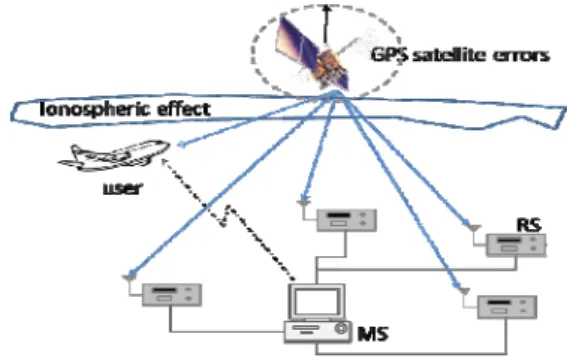
(28) Implementation of the Wide Area Differential GPS Master Station Algorithms in Taipei Flight Information Region Shih-Chieh Lu and Shau-Shiun Jan* Institute of Civil Aviation, National Cheng Kung University, Tainan 70101, Taiwan (Tel: +886-6-2349294, E-mail: [email protected]). Abstract: This paper implements the Wide Area Differential GPS (WADGPS) master station algorithms to facilitate the operation of a satellite based aviation navigation system in Taipei Flight Information Region (FIR). The WADGPS master station algorithms used in this paper are based on that of the National Satellite Test Bed (NSTB) operated by Federal Aviation Administration (FAA). The master station processes include the GPS L1-L2 dual frequency observation data collector, the ionospheric delay estimation module, and the satellite ephemeris and clock error estimation modules. At first, the data collector checks for the reasonableness of Signal-to-Noise Ratio (SNR) for each satellite in view, and it also implements the dual frequency carrier smooth to reduce the code noise and multipath effects. The ionospheric delay model used in this work is a thin shell model at the altitude of 350 km above the earth surface, and the planar fit method is implemented to generate the ionospheric grid model based on the L1-L2 dual frequency observation data. Furthermore, the pseudorange residuals from the reference stations to satellites are synchronized to a common clock by the Common View Time Transfer (CVTT). These synchronized residuals are used to estimate the satellites ephemeris and clock errors by the minimum-variance method. This master station provides the differential positioning services to users, and the confidence bounds of these correction messages which will be computed by the protection level calculation. To validate the implemented WADGPS master station algorithms, this paper uses the archive data from NSTB reference stations to generate the WADGPS corrections and then compare them with the archive WAAS correction messages provided by the FAA WAAS website. After the validation processes, this paper uses the local reference stations which are e-GPS observation stations operated by the Ministry of Interior (MOI) in Taiwan to evaluate the performance of WADGPS in Taipei Flight Information Region.. Keywords: WADGPS, NSTB, the integrity messages. 1. Introduction The Global Positioning System (GPS) provides positioning, navigation and timing services for several applications. However, GPS without the monitoring system cannot provide the service for civil aviation users. Therefore, an augmentation system is essential for GPS to supply a comprehensive service to civil aviation users. As a result, the goal of this paper is to develop a Wide Area Differential GPS (WADGPS) to enhance the GPS performance for civil aviation users in Taipei Flight Information Region (FIR). The WADGPS is guaranteed to provide service which satisfies the safety requirements of certain phases of flight to civil aviation users [1]. The WADGPS developed in this work consists of a Master Station (MS) and several Reference Stations (RS) [2]. The GPS dual frequency measurements collected by each local RS are transmitted to the master station. The master station generates vector corrections for satellite ephemeris and clock errors, and ionospheric delays, as shown in Figure 1 [3]. Finally, the WADGPS messages can be transmitted to users via radio, Internet, or GEO. Similar to this work, the Federal Aviation Administration (FAA) implemented the National Satellite Test Bed (NSTB) as a prototype system to evaluate the. Wide Area Augmentation System (WAAS) algorithms [4]. The WADGPS master station algorithms developed in this paper are based on the NSTB algorithms. As for the WADGPS reference stations, the e-GPS observation stations built by Ministry of Interior (MOI) in Taiwan are used to be the reference stations to collect the dual frequency GPS data.. Figure 1. The Wide Area Differential GPS This paper focuses on the implementation of the WADGPS master station algorithms. Accordingly, this paper is organized as follows: Section 2 describes the details of the WADGPS.

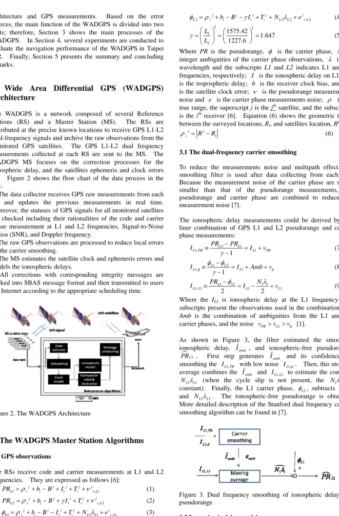
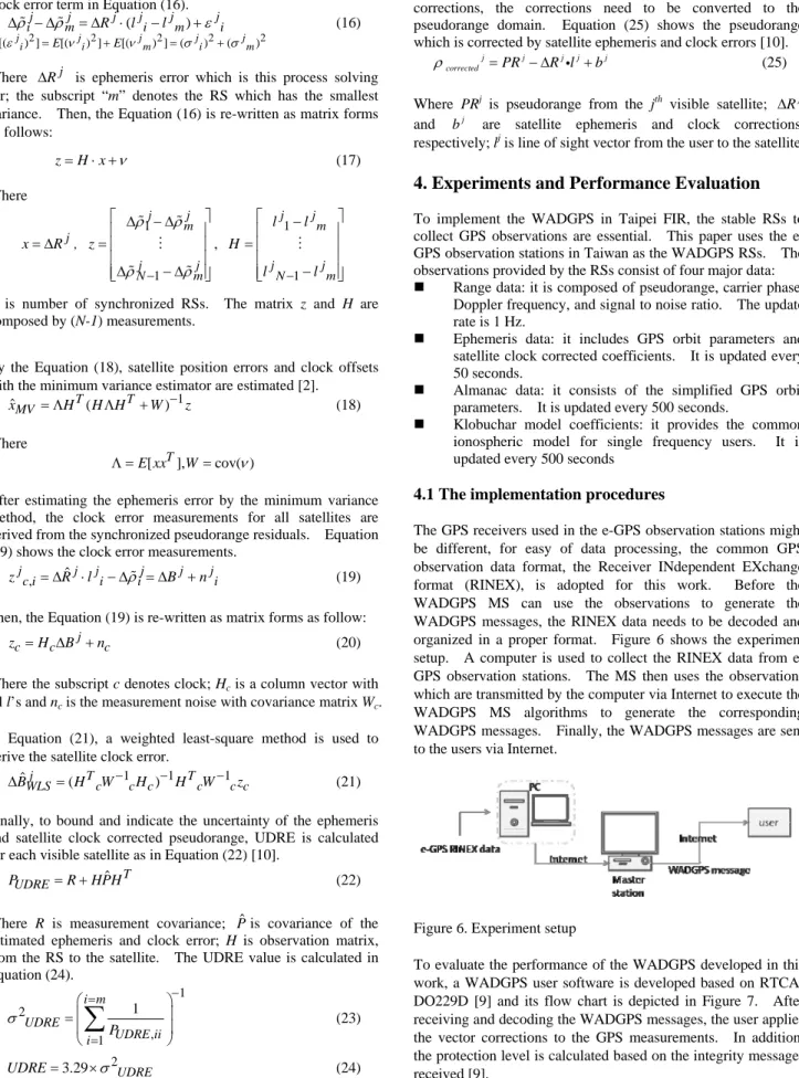
(29) architecture and GPS measurements. Based on the error sources, the main function of the WADGPS is divided into two parts; therefore, Section 3 shows the main processes of the WADGPS. In Section 4, several experiments are conducted to evaluate the navigation performance of the WADGPS in Taipei FIR. Finally, Section 5 presents the summary and concluding remarks.. 2. Wide Area Differential GPS (WADGPS) Architecture The WADGPS is a network composed of several Reference Stations (RS) and a Master Station (MS). The RSs are distributed at the precise known locations to receive GPS L1-L2 dual-frequency signals and archive the raw observations from the monitored GPS satellites. The GPS L1-L2 dual frequency measurements collected at each RS are sent to the MS. The WADGPS MS focuses on the correction processes for the ionospheric delay, and the satellites ephemeris and clock errors [5]. Figure 2 shows the flow chart of the data process in the MS: 1. The data collector receives GPS raw measurements from each RS and updates the previous measurements in real time. Moreover, the statuses of GPS signals for all monitored satellites are checked including their rationalities of the code and carrier phase measurement at L1 and L2 frequencies, Signal-to-Noise Ratios (SNR), and Doppler frequency. 2. The raw GPS observations are processed to reduce local errors by the carrier smoothing. 3. The MS estimates the satellite clock and ephemeris errors and models the ionospheric delays. 4. All corrections with corresponding integrity messages are packed into SBAS message format and then transmitted to users via Internet according to the appropriate scheduling time.. φL 2 = ρ i j + bi − B j − γ I i j + Ti j + N L 2λL 2 + e j i , L 2 2. ⎛ L1 ⎞ ⎛ 1575.42 ⎞ ⎟ =⎜ ⎟ = 1.647 ⎝ L2 ⎠ ⎝ 1227.6 ⎠. (4). 2. γ =⎜. (5). Where PR is the pseudorange, φ is the carrier phase, N is integer ambiguities of the carrier phase observations, λ is the wavelength and the subscripts L1 and L2 indicates L1 and L2 frequencies, respectively; I is the ionospheric delay on L1; T is the tropospheric delay; b is the receiver clock bias, and B is the satellite clock error; ν is the pseudorange measurements noise and e is the carrier phase measurements noise; ρ is the true range, the superscript j is the jth satellite, and the subscript i is the ith receiver [6]. Equation (6) shows the geometric range between the surveyed locations, Ri, and satellites location, Rj. ρ i j = R j − Ri (6) 3.1 The dual-frequency carrier smoothing To reduce the measurements noise and multipath effect, the smoothing filter is used after data collecting from each RS. Because the measurement noise of the carrier phase are much smaller than that of the pseudorange measurements, the pseudorange and carrier phase are combined to reduce the measurement noise [7]. The ionospheric delay measurements could be derived by the liner combination of GPS L1 and L2 pseudorange and carrier phase measurements: PRL 2 − PRL1 (7) I L1, PR ≡ = I L1 + vPR γ −1 φ −φ I L1,φ ≡ L1 L 2 = I L1 + Amb + vφ (8) γ −1 PRL1 − φL1 Nλ (9) I L1, L1 ≡ = I L1 − 1 1 + vL1 2 2 Where the IL1 is ionospheric delay at the L1 frequency; the subscripts present the observations used in the combination; the Amb is the combination of ambiguities from the L1 and L2 carrier phases, and the noise vPR > vL1 > vφ [1]. As shown in Figure 3, the filter estimated the smoothed ionospheric delay, Iˆsmth , and ionospheric-free pseudorange, PR L1 . First step generates Iˆsmth and its confidence by smoothing the I L1, PR with low noise I L1,φ . Then, this moving average combines the Iˆsmth and I L1, L1 to estimate the constant N L1λL1 (when the cycle slip is not present, the N1λ1 is constant). Finally, the L1 carrier phase, φL1 , subtracts Iˆsmth and N L1λL1 . The ionospheric-free pseudorange is obtained. More detailed description of the Stanford dual frequency carrier smoothing algorithm can be found in [7].. Figure 2. The WADGPS Architecture. 3. The WADGPS Master Station Algorithms 3.1 GPS observations The RSs receive code and carrier measurements at L1 and L2 frequencies. They are expressed as follows [6]: PRL1 = ρ i j + bi − B j + I i j + Ti j + ν j i , L1 (1). PRL 2 = ρ i j + bi − B j + γ I i j + Ti j + ν j i , L 2. (2). φL1 = ρ i j + bi − B j − I i j + Ti j + N L1λL1 + e j i , L1. (3). Figure 3. Dual frequency smoothing of ionospheric delay and pseudorange 3.2 Ionospheric delay model.

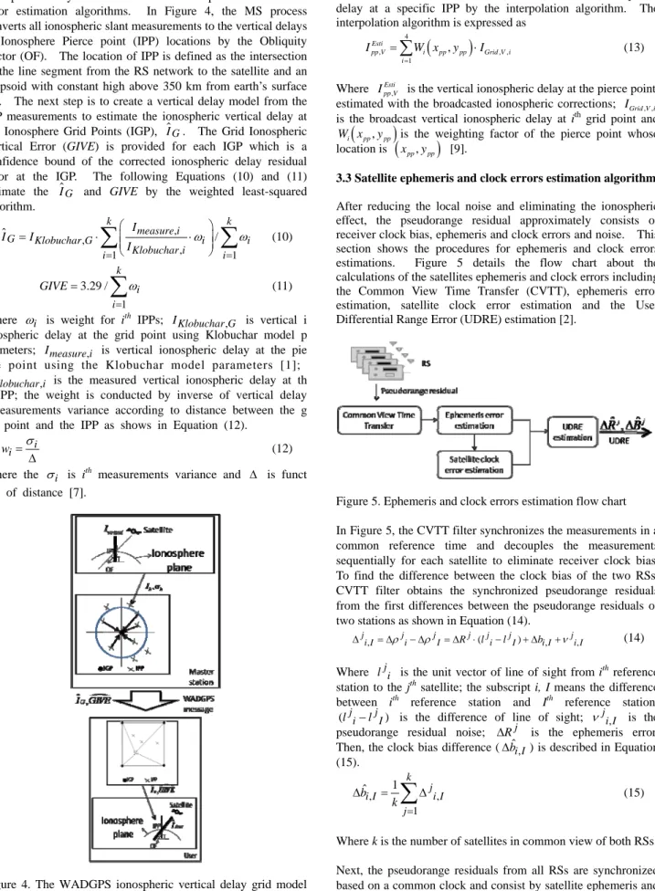
(30) The major functions of the WADGPS master station are the ionospheric delay model and the satellites ephemeris and clock error estimation algorithms. In Figure 4, the MS process converts all ionospheric slant measurements to the vertical delays at Ionosphere Pierce point (IPP) locations by the Obliquity Factor (OF). The location of IPP is defined as the intersection of the line segment from the RS network to the satellite and an ellipsoid with constant high above 350 km from earth’s surface [8]. The next step is to create a vertical delay model from the IPP measurements to estimate the ionospheric vertical delay at the Ionosphere Grid Points (IGP), I G . The Grid Ionospheric Vertical Error (GIVE) is provided for each IGP which is a confidence bound of the corrected ionospheric delay residual error at the IGP. The following Equations (10) and (11) estimate the I G and GIVE by the weighted least-squared algorithm. k ⎛ I measure,i. ⎞ k I G = I Klobuchar ,G ⋅ ⋅ ωi ⎟ / ωi ⎜ ⎜ I Klobuchar ,i ⎟ ⎝ ⎠ i =1 i =1. ∑. ∑. (10). k. GIVE = 3.29 /. ∑ωi. (11). i =1. Where ωi is weight for ith IPPs; I Klobuchar ,G is vertical i onospheric delay at the grid point using Klobuchar model p arameters; I measure,i is vertical ionospheric delay at the pie rce point using the Klobuchar model parameters [1]; I Klobuchar ,i is the measured vertical ionospheric delay at th e IPP; the weight is conducted by inverse of vertical delay measurements variance according to distance between the g rid point and the IPP as shows in Equation (12).. σ (12) wi = i Δ Where the σ i is ith measurements variance and Δ is funct ion of distance [7].. The bottom plot of Figure 4 describes that the user uses the nearest IGPs around the IPP to estimate the vertical ionospheric delay at a specific IPP by the interpolation algorithm. The interpolation algorithm is expressed as Esti I pp ,V = ∑ Wi ( x pp , y pp ) ⋅ I Grid ,V , i 4. (13). i =1. Esti Where I pp ,V is the vertical ionospheric delay at the pierce point, estimated with the broadcasted ionospheric corrections; I Grid ,V ,i is the broadcast vertical ionospheric delay at ith grid point and Wi ( x pp , y pp ) is the weighting factor of the pierce point whose location is ( x pp , y pp ) [9].. 3.3 Satellite ephemeris and clock errors estimation algorithm. After reducing the local noise and eliminating the ionospheric effect, the pseudorange residual approximately consists of receiver clock bias, ephemeris and clock errors and noise. This section shows the procedures for ephemeris and clock errors estimations. Figure 5 details the flow chart about the calculations of the satellites ephemeris and clock errors including the Common View Time Transfer (CVTT), ephemeris error estimation, satellite clock error estimation and the User Differential Range Error (UDRE) estimation [2].. Figure 5. Ephemeris and clock errors estimation flow chart In Figure 5, the CVTT filter synchronizes the measurements in a common reference time and decouples the measurements sequentially for each satellite to eliminate receiver clock bias. To find the difference between the clock bias of the two RSs, CVTT filter obtains the synchronized pseudorange residuals from the first differences between the pseudorange residuals of two stations as shown in Equation (14). (14) Δ j i , I = Δρ j i − Δρ j I = ΔR j ⋅ (l j i − l j I ) + Δbi , I + ν j i, I Where l j i is the unit vector of line of sight from ith reference station to the jth satellite; the subscript i, I means the difference between ith reference station and Ith reference station; (l j i − l j I ) is the difference of line of sight; ν j i, I is the pseudorange residual noise; ΔR j is the ephemeris error. Then, the clock bias difference ( Δbˆi, I ) is described in Equation (15). Δbˆi , I =. 1 k. k. ∑ Δ ji, I. (15). j =1. Where k is the number of satellites in common view of both RSs.. Figure 4. The WADGPS ionospheric vertical delay grid model flow chart. Next, the pseudorange residuals from all RSs are synchronized based on a common clock and consist by satellite ephemeris and clock error. The ephemeris error and the clock error have to be.

(31) sent frequently, and it occupies lots of bandwidth. To reduce the bandwidth, separating the satellite clock error term is necessary. The single difference is used to remove the satellite clock error term in Equation (16). Δρ ij − Δρ mj = ΔR j ⋅ (l j i − l j m ) + ε j i (16) E[(ε j i ) 2 ] = E[(ν j i ) 2 ] + E[(ν j m ) 2 ] = (σ j i ) 2 + (σ j m )2. Where ΔR j is ephemeris error which is this process solving for; the subscript “m” denotes the RS which has the smallest variance. Then, the Equation (16) is re-written as matrix forms as follows: z = H ⋅ x +ν. Where PUDRE ,ii is the ith diagonal element of the PUDRE. When the users receive the satellite ephemeris and clock corrections, the corrections need to be converted to the pseudorange domain. Equation (25) shows the pseudorange which is corrected by satellite ephemeris and clock errors [10]. ρ corrected j = PR j − ΔR j il j + b j (25) Where PRj is pseudorange from the jth visible satellite; ΔR j and b j are satellite ephemeris and clock corrections, respectively; lj is line of sight vector from the user to the satellite.. (17). 4. Experiments and Performance Evaluation. Where ⎡ Δρ j − Δρ j ⎤ ⎡ l j −l j ⎤ 1 m ⎥ m ⎥ ⎢ ⎢ 1 x = ΔR , z = ⎢ ⎥, H =⎢ ⎥ ⎢ j ⎢ j j ⎥ j ⎥ ⎢⎣l N −1 − l m ⎦⎥ ⎣⎢ Δρ N −1 − Δρ m ⎦⎥ j. N is number of synchronized RSs. The matrix z and H are composed by (N-1) measurements.. By the Equation (18), satellite position errors and clock offsets with the minimum variance estimator are estimated [2]. xˆMV = ΛH T ( H ΛH T + W )−1 z (18) Where Λ = E[ xxT ],W = cov(ν ). After estimating the ephemeris error by the minimum variance method, the clock error measurements for all satellites are derived from the synchronized pseudorange residuals. Equation (19) shows the clock error measurements. z j = ΔRˆ j ⋅ l j − Δρ j = ΔB j + n j (19) c,i. i. i. i. Then, the Equation (19) is re-written as matrix forms as follow: zc = H c ΔB j + nc. (20). Where the subscript c denotes clock; Hc is a column vector with all l’s and nc is the measurement noise with covariance matrix Wc. In Equation (21), a weighted least-square method is used to derive the satellite clock error. j ΔBˆ WLS = ( H T cW −1c H c ) −1 H T cW −1c zc (21). To implement the WADGPS in Taipei FIR, the stable RSs to collect GPS observations are essential. This paper uses the eGPS observation stations in Taiwan as the WADGPS RSs. The observations provided by the RSs consist of four major data: Range data: it is composed of pseudorange, carrier phase, Doppler frequency, and signal to noise ratio. The update rate is 1 Hz. Ephemeris data: it includes GPS orbit parameters and satellite clock corrected coefficients. It is updated every 50 seconds. Almanac data: it consists of the simplified GPS orbit parameters. It is updated every 500 seconds. Klobuchar model coefficients: it provides the common ionospheric model for single frequency users. It is updated every 500 seconds. 4.1 The implementation procedures The GPS receivers used in the e-GPS observation stations might be different, for easy of data processing, the common GPS observation data format, the Receiver INdependent EXchange format (RINEX), is adopted for this work. Before the WADGPS MS can use the observations to generate the WADGPS messages, the RINEX data needs to be decoded and organized in a proper format. Figure 6 shows the experiment setup. A computer is used to collect the RINEX data from eGPS observation stations. The MS then uses the observations which are transmitted by the computer via Internet to execute the WADGPS MS algorithms to generate the corresponding WADGPS messages. Finally, the WADGPS messages are sent to the users via Internet.. Finally, to bound and indicate the uncertainty of the ephemeris and satellite clock corrected pseudorange, UDRE is calculated for each visible satellite as in Equation (22) [10]. ˆ T PUDRE = R + HPH (22) Where R is measurement covariance; Pˆ is covariance of the estimated ephemeris and clock error; H is observation matrix, from the RS to the satellite. The UDRE value is calculated in Equation (24). ⎛ i =m. ⎞ ⎟ ⎟ P ⎝ i =1 UDRE ,ii ⎠. σ 2UDRE = ⎜ ⎜. ∑. 1. UDRE = 3.29 × σ 2UDRE. −1. (23) (24). Figure 6. Experiment setup To evaluate the performance of the WADGPS developed in this work, a WADGPS user software is developed based on RTCADO229D [9] and its flow chart is depicted in Figure 7. After receiving and decoding the WADGPS messages, the user applies the vector corrections to the GPS measurements. In addition, the protection level is calculated based on the integrity messages received [9]..

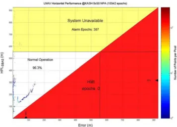
(32) Horizontal Error Plot (NPA) Bound by 3.9σ. 1000. North (m). 500. 0. -500. Figure 7. The procedures of the WADGPS user software The way to apply the WADGPS corrections in positioning is illustrated briefly in Equations (12) and (24) of Section 3. The Horizontal Protection Level (HPL) calculation is defined in RTCA DO-229D [9].. -1000 -1000. -500. 0 East (m). 500. 1000. Figure 9. The horizontal positioning error and error bound. 4.2 The analysis of experiment result In this paper, three e-GPS observation stations are used to be the RSs, and one e-GPS observation station is utilized as a user. Figure 8 illustrates the distribution of the e-GPS observation stations used in this work; the blue markers indicate the RSs, and the yellow marker shows the user.. Figure 10. The vertical positioning error and error bound. Figure 8. The e-GPS observation stations distribution Figures 9 and 10 show the positioning error distributions after applying the WADGPS corrections in positioning. For the horizontal positioning result shown in Figure 9, the outer circle indicates the error bound on all the horizontal position solutions and the inner circle indicates the 95% (i.e., 2σ ) error bound on the horizontal position solutions; the 95% error bound is 84.5 m. The vertical position error distribution is shown in Figure 10. Similarly, the vertical position errors are within 3.9 σ error bound. The results are influenced by the number of satellites in view of the RSs. Because of the limited RSs used in this work, the number of satellites in positioning is occasionally less than five. Therefore, those epochs would have large positioning error, as shown in Figures 9 and 10. The top plot of Figure 11 shows the horizontal positioning error and the corresponding HPL values, and the number of satellites used in positioning is shown in the bottom plot. As shown in Figure 11, when the number of positioning satellites downs to four, the HPL values are larger than the horizontal positioning error.. Figure 11. The HPL values (top) and the number of satellites used in positioning (bottom) Figure 12 shows the LNAV performance of the developed WADGPS on the Stanford Chart [11] [12]. The definition of Stanford Chart is detailed in [11]. In Figure 12, 96% of the epochs are in normal operation for the LNAV requirement (i.e., Horizontal Alert Limit (HAL) = 556 m), importantly, all epochs are not in the HMI region. As a result, the WADGPS developed in this work could provide the integrity service in this experiment..

(33) Navstar GPS Space Segment/User Interfaces, IRN200C-002, Navstar GPS JPO, 25 September 1997. [7] Y.C. Chao, “Real Time Implementation of the Wide Area Augmentation System for the Global Position System with an Emphasis on Ionospheric Modeling,” Department of Aeronautics and Astronautics Thesis, Stanford University, 1997. [8] Y.C. Chao, Y.J. Tsai, T. Walter, C. Kee, et.al., "The Ionospheric Delay Model Improvement for the Stanford WAAS Network," Proceedings of ION National Technical Meeting 95, Anaheim, CA., Jan. 18-20, 1995. [9] WAAS MOPS (Minimum Operational Performance Standards for global positioning system/ Wide Area Augmentation System airborne equipment), RTCA/DO-229D. [10] C. Kee, Y. Yun, and D. Kim, "Simulation-based Performance Analysis of SBAS in Korea: Accuracy & Availability," Proceedings of ION GPS/GNSS 2003, Portland, OR., Sep. 9-12, 2003. [11] The GPS lab web site of Stanford University, http://waas.stanford.edu/index.html. [12] R.J. Kelly, J.M. Davis, “Required Navigation Performance (RNP) for Precision Approach and Landing GNSS Application,” Navigation, Journal of the Institute of Navigation, Vol. 41, No. 1, Spring 1994.. [6]. Figure 12. The LNAV (NPA) performance of the developed WADGPS on the Stanford Chart. 5. Conclusions This paper implemented the Wide Area Differential GPS (WADGPS) master station algorithms to facilitate the operation of a satellite based aviation navigation system in Taipei Flight Information Region (FIR). The WADGPS master station algorithms used in this paper are based on that of the National Satellite Test Bed (NSTB) operated by Federal Aviation Administration (FAA). The e-GPS observation stations operated by the Ministry of Interior, Taiwan are used as our WADGPS Reference Stations (RSs). As part of this work, a WADGPS user software is developed to investigate the LNAV (NPA) performance of the implemented WADGPS. As shown in the experiment results, the WADGPS developed in this work could provide the enhanced positioning service with integrity to civil aviation users within Taipei Flight Information Region (FIR). The next step is to extend the reference stations in this WADGPS network to further enhance its performance.. Acknowledgement The work presented in this paper is supported by Taiwan National Science Council under the research grant NSC 982221-E-006- 1 2 2 . The authors gratefully acknowledge this support.. Reference [1] [2]. [3]. [4]. [5]. B.W. Parkinson, J.J. Spilker, Global Positioning System: Theory and Application, AIAA Publication, 1996. P. Enge, T. Walter, S. Pullen, C. Kee, Y.C. Chao, and Y.J. Tsai, “Wide Area Augmentation of the Global Positioning System,” Proceedings of the IEEE, 1996. Y.J. Tsai, Wide Area Differential Operation of the Global Positioning System: Ephemeris and Clock Algorithms, Department of Aeronautics and Astronautics Thesis, Stanford University, 1999. R.A. Fuller, “Aviation Utilization of Geostationary Satellites for the Augmentation to GPS: Ranging and Data Link,” Department of Aeronautics and Astronautics Thesis, Stanford University, 2000. C. Kee, “Wide Area Differential GPS (WADGPS),” Department of Aeronautics and Astronautics Thesis, Stanford University, 1993..

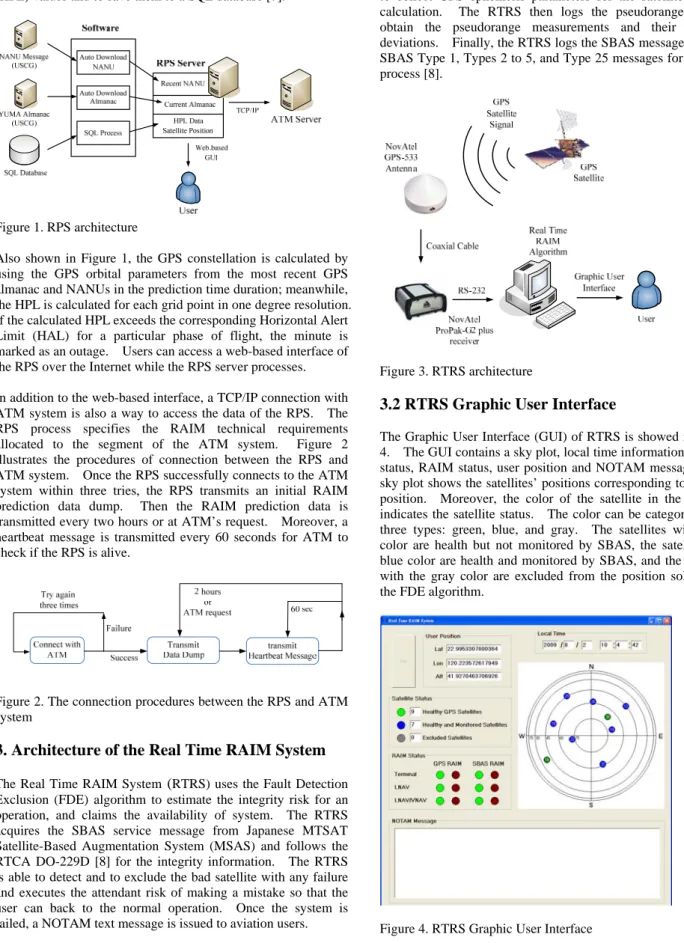
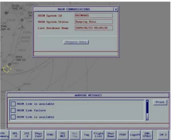
(34) Development and Implementation of RAIM to Support the New ATM System Shou-Ju Yeh and Shau-Shiun Jan*. Institute of Civil Aviation, National Cheng Kung University, Tainan 70101, Taiwan (Tel: +886-6-2349294, E-mail: [email protected]). Abstract:. Civil aviation organizations around the world are implementing the next generation Communication, Navigation, Surveillance, and Air Traffic Management (CNS/ATM) systems to meet the needs of future aviation transportations. One of the key enabling technologies of the CNS/ATM system is the use of Global Positioning System (GPS). According to the AC 90-100A published by Federal Aviation Administration (FAA), it requires the operators to check the GPS Receiver Autonomous Integrity Monitoring (RAIM) availability for the intended route of flight if the TSO-C129 equipment is used to solely satisfy the Area Navigation (RNAV) requirements. Therefore, we at the Institute of Civil Aviation of National Cheng Kung University work with Taiwan Civil Aeronautics Administration (CAA) to develop a RAIM Prediction System (RPS) to provide the 72-hour RAIM prediction information over Taipei Flight Information Region (FIR) to support the ATM system. Furthermore, as for monitoring the unscheduled faults of GPS for specific airport in Taipei FIR, we also develop a real time RAIM system (RTRS) for airport operators.. Keywords: Global Positioning System (GPS), Integrity, Receiver Autonomous Integrity Monitoring (RAIM). 1. Introduction Nowadays, the augmented Global Positioning System (GPS) is generally used for the safety-of-life applications such as the Air Traffic Management (ATM) system. The service of Required Navigation Performance (RNP) provided by GPS is essential for civil aviation users. The integrity directly is considered as a critical element of the RNP parameters and relates to the safety. Any potentially hazardous or misleading piece of information has to be flagged before it leads to a positioning error. However, the integrity information provided by the navigation message from GPS is not timely enough for the safety-of-life applications. For this purpose, the Receiver Autonomous Integrity Monitoring (RAIM) system is implemented for the ATM system to provide the assurance of integrity [1]. In addition, civil aviation organizations around the world are implementing the next generation of Communication, Navigation, Surveillance, and Air Traffic Management (CNS/ATM) systems to meet the needs of future aviation transportations. The Civil Aeronautics Administration (CAA) in Taiwan is executing the CNS/ATM program to improve the capacity of airports and the efficiency of flight. This new CNS/ATM system integrating the interfaces of present systems provides the services of the air traffic control system, the air traffic flow management, and the airspace management. One of the keys to enable technologies of the CNS/ATM system is the use of GPS [2]. Therefore, the CNS/ATM system which uses GPS as the supplemental equipment is required to satisfy the specifically international regulations. According to the Advisory Circular (AC) 90-100A [3] published on March 1st, 2007 by Federal Aviation Administration (FAA), the operators is demanded to check the GPS RAIM availability for the intended route of flight if the Technical Standard Order (TSO)-C129 [4] equipment is used to solely satisfy the Area Navigation (RNAV) requirements. Therefore, for the users of Taipei Flight Information Region (FIR), a RAIM Prediction. System (RPS) through the cooperation with Taiwan CAA is developed to provide the 72-hour RAIM prediction information. However, to exclude every potential failure during the whole stages [5], the Real Time RAIM System (RTRS,) a mechanism to prevent the integrity failure caused by those faults, is further established to detect unscheduled faults of GPS and guarantee the safety-of-life applications in airport. As a result, the operators in specific airport within Taipei FIR are capable of catching the predicted and real time integrity information. The objective of this work is to develop and implement the RAIM system for aviation applications. Accordingly, the second section begins with the description of the RPS architecture. The third section will introduce the architecture and the graphic user interface of the RTRS. In the fourth section, the development and implementation results of the RPS and the RTRS will be evaluated. Finally, this work will be concluded in the fifth section.. 2. Architecture of the RAIM Prediction System The RPS uses GPS YUMA almanac to predetermine GPS satellite constellation and indicates any change of the GPS satellite status by the Notice Advisory to NAVSTAR User (NANU) [6]. The RPS points out the areas of the affected airspace where any satellite is taken out of service for maintenance. Additionally, the RPS provides the prediction information via a TCP/IP connection to the ATM system. The RPS architecture is shown in Figure 1. In figure 1, there are three software processes, namely, the automatically download almanac process, the automatically download NANU process, and the SQL process. The first software process is capable to routinely acquire the YUMA almanacs every 12 hours. The second software is designed to obtain the latest NANU every 2 hours. The RPS server gets both almanac and NANU information from the United States Coast Guard (USCG) server [6]. The third software is used to determine the GPS.

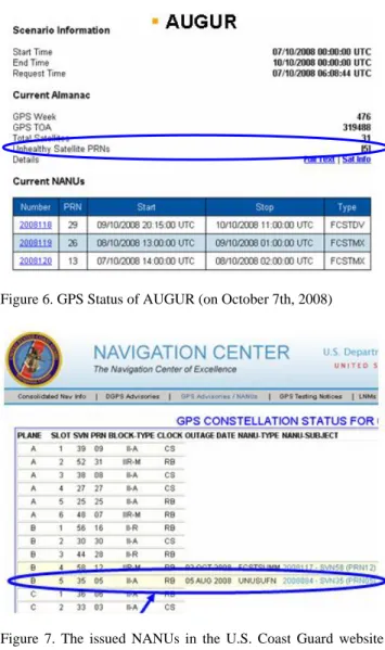
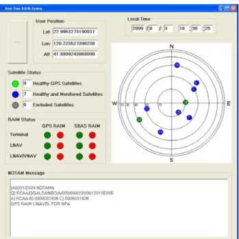
(35) constellation and the corresponding Horizontal Protection Level (HPL) values and to save them to a SQL database [7].. observation data. First, the RTRS logs the GPS ephemeris data to collect GPS ephemeris parameters for the satellite position calculation. The RTRS then logs the pseudorange data to obtain the pseudorange measurements and their standard deviations. Finally, the RTRS logs the SBAS messages such as SBAS Type 1, Types 2 to 5, and Type 25 messages for the FDE process [8].. Figure 1. RPS architecture Also shown in Figure 1, the GPS constellation is calculated by using the GPS orbital parameters from the most recent GPS almanac and NANUs in the prediction time duration; meanwhile, the HPL is calculated for each grid point in one degree resolution. If the calculated HPL exceeds the corresponding Horizontal Alert Limit (HAL) for a particular phase of flight, the minute is marked as an outage. Users can access a web-based interface of the RPS over the Internet while the RPS server processes. In addition to the web-based interface, a TCP/IP connection with ATM system is also a way to access the data of the RPS. The RPS process specifies the RAIM technical requirements allocated to the segment of the ATM system. Figure 2 illustrates the procedures of connection between the RPS and ATM system. Once the RPS successfully connects to the ATM system within three tries, the RPS transmits an initial RAIM prediction data dump. Then the RAIM prediction data is transmitted every two hours or at ATM’s request. Moreover, a heartbeat message is transmitted every 60 seconds for ATM to check if the RPS is alive.. Figure 3. RTRS architecture. 3.2 RTRS Graphic User Interface The Graphic User Interface (GUI) of RTRS is showed in Figure 4. The GUI contains a sky plot, local time information, satellite status, RAIM status, user position and NOTAM message. The sky plot shows the satellites’ positions corresponding to the user position. Moreover, the color of the satellite in the sky plot indicates the satellite status. The color can be categorized into three types: green, blue, and gray. The satellites with green color are health but not monitored by SBAS, the satellite with blue color are health and monitored by SBAS, and the satellites with the gray color are excluded from the position solution by the FDE algorithm.. Figure 2. The connection procedures between the RPS and ATM system. 3. Architecture of the Real Time RAIM System The Real Time RAIM System (RTRS) uses the Fault Detection Exclusion (FDE) algorithm to estimate the integrity risk for an operation, and claims the availability of system. The RTRS acquires the SBAS service message from Japanese MTSAT Satellite-Based Augmentation System (MSAS) and follows the RTCA DO-229D [8] for the integrity information. The RTRS is able to detect and to exclude the bad satellite with any failure and executes the attendant risk of making a mistake so that the user can back to the normal operation. Once the system is failed, a NOTAM text message is issued to aviation users.. 3.1 Architecture of the RTRS The RTRS architecture is shown in Figure 3. This work uses a NovAtel ProPak-G2-plus GPS receiver to collect GPS. Figure 4. RTRS Graphic User Interface If the number of SBAS-monitored satellites is greater than four, the SBAS-monitored satellites are used by RTRS to provide the positioning service; otherwise, the SBAS RAIM would be unavailable. The user time information is the local time.

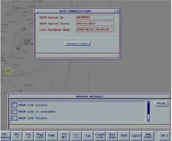
(36) acquired from the user computer. The RAIM status indicates whether the RAIM is available for the specific phase of flight. For each HPL calculation, the green lights indicate that the HPL is below the specific HAL of different requirements. The user position is showed in longitude, latitude, and altitude coordinate system. If any faulty satellite is excluded successfully, RTRS recalculates the user position with the remaining satellites; otherwise, a NOTAM message appears in the NOTAM message window to notice the users.. 4. Performance Evaluations of the RPS and the RTRS In the RPS performance evaluation, the proposed RPS is compared with EUROCONTROL AUGUR system developed by EUROCONTROL, and the airports used in the comparison are Taiwan Taoyuan International Airport and Kaohsiung International Airport. The comparison of output from the AUGUR and RPS GPS status tools which are inputs to RAIM algorithms is provided. Furthermore, this section would describe the user-friendly interface that has been developed for the RPS.. Figure 6. GPS Status of AUGUR (on October 7th, 2008). 4.1 The GPS Status Page of the RPS As shown in Figure 5, GPS status page provides the information including “Scenario Information,” “Current Almanac,” and “Current NANU” for the next 72 hours. “Scenario Information” in GPS Status page comprises three time tags: “Start Time,” “End Time,” and “Request Time.” “Start Time” and “End Time” indicate the RPS prediction duration. “Request Time” is the time that user accesses this website. “Current Almanac” describes the GPS week, the Time Of Applicability (TOA) of current YUMA almanac, and the number of satellites in current YUMA almanac. “Current NANU” shows the information of scheduled satellite outage if the outage is within the prediction duration. The GPS status information from RPS and AUGUR are checked on specific days to compare with the actual GPS constellation from the status page of the U.S. Coast Guard Navigation Center [6]. Figures 5 and 6 provide the summary of the GPS status comparison on October 7th, 2008. In Figures 5 and 6, both RPS and AUGUR indicate three NANUs, 2008118, 2008119, 2008120. However, NANU 2008084 was only pointed out by the RPS as shown in Figure 6 because AUGUR marked PRN 5 as an unhealthy satellite. According to the U.S. Coast Guard website, as shown in Figure 7, the NANU 2008084 message was issued for the PRN05 outage until further notice.. Figure 7. The issued NANUs in the U.S. Coast Guard website (on October 7th, 2008). 5.2 The NPA Tool Page of the RPS “NPA Tool” is available for users to view RAIM prediction information at Taoyuan International Airport (ICAO code: RCTP) or Kaohsiung International Airport (ICAO code: RCKH) over the next 72 hours, and the prediction results are displayed in either a graphic or text format. In graphic format, the prediction results display in a bar chart. The horizontal axis of the bar indicates the corresponding prediction time, and the line width represents the time duration. To distinguish the outages, NPA Tool marks the outage epoch as a red line; otherwise, it is marked as a gray line. In text format, the message includes four parts: “Scenario Information,” “Configuration,” “Constellation,” and “Outage Information.” “Scenario Information” in the NPA Tool page and GPS status page are the same. “Configuration” indicates the mask angle used in the prediction. “Constellation” lists the current YUMA almanac and NANU information. “Outage Information” describes the outage epoch by a string of text messages. Both AUGUR website and RPS are able to provide NPA RAIM analysis for Taoyuan (ICAO code: RCTP) and Kaohsiung (ICAO code: RCKH) International Airports. The scenarios for this analysis are:. Figure 5. GPS Status of the RPS (on October 7th, 2008). z. Analysis period – October 27th to 29th, 2008.