Research Express@NCKU - Articles Digest
Research Express@NCKU Volume 7 Issue 10 - March 13, 2009
[ http://research.ncku.edu.tw/re/articles/e/20090313/2.html ]
Monitoring Long-Memory Air Quality Data
Using ARFIMA Model
Jeh-Nan Pan
1,*and Su-Tsu Chen
21Department of Statistics, National Cheng-Kung University, Tainan, Taiwan, R.O.C.
2Science Education Center, Fooyin University, Kaohsiung Hsien, Taiwan, R.O.C.
ENVIRONMETRICS 2008, 19, 209-219
U
nlike the traditional control charts in whichobservations are assumed to be independent, observations of air quality and other environmental processes usually have autocorrelations. For example, PM10 (particles between 2.5 and 10 micrometers) and O3 of air quality in the Taipei city follow the autoregressive integrated moving average (ARIMA) models. When applying control chart to
autocorrelated data, it is commonly assumed that statistical models and white noises could fit the data. After fitting an appropriate model to the data, the residuals can be calculated. If the model is suitable, residuals should be independently and identically normally distributed and
residual control charts can be applied then. If the control chart gives a signal, the process will be intervened and necessary corrective actions need to be taken.
Autocorrelated data usually have significant autocorrelation functions just for small lags. However, the air pollution data have significant autocorrelation functions even at a very large lag due to the property of long-memory processes. Usually, there are two phases of constructing the residual control chart for fractionally integrated autoregressive moving average (ARFIMA) model. “Phase I” is to establish control limits using a historical data set. “Phase II” is the period of using these limits to monitor the process. If control charts signal, operators should step in to bring processes back to in-control state. Listed below are the proposed procedures for constructing control limits for the control chart using ARFIMA models in Phase I.
1.Collect historical air quality or environmental data.
2.Fit the data collected in step 1 into an appropriate model and perform estimation of parameters. Check the suitability of the model. After a proper model is selected, residuals can be calculated.
3.Establish control limits for the residuals.
4.Delete any residuals fallen beyond the control limits and estimate parameters of control charts. 5.Reestablish control limits for the residuals.
Research Express@NCKU - Articles Digest
6.Repeat step 4 and step 5 until there are no outliers/out-of-control signals.
If models and parameters of processes are known in advance, then the control limits could be calculated and one can bypass the Phase I. The control limits established in Phase I are used to monitor processes in Phase II. The above procedures help in constructing an appropriate chart using ARFIMA models. The application of the above procedures will be demonstrated by the following empirical example of long-memory air quality data of southern Taiwan.
There are 58 surveillance stations established by EPA of Taiwan to monitor the air quality in Taiwan. The largest industrial city, Kaohsiung, located in the southern Taiwan, has serious air pollution problems. Nantsz is an administrative district in Kaohsiung city, where a big refinery plant of Chinese Petroleum Corporation and many other industries locate there. It is also well known for a long history of public protest for pollution. The air quality data of PM10 collected by Nantsz station are discussed in this paper since PM10 is the important index to health as mentioned in section 2. The hourly data were collected between 1999 and 2002 by Nantsz station. In this example, daily average is used and we drop some missing data due to measurement failure or unbelievable measurement. Thus, a total 725
observations were recorded during 1999 to 2000 and 712 observations were recorded between 2001 and 2002.
There are two phases for the construction of control charts. In Phase I, a set of historical data is chosen and parameters of the fitted model are estimated. In this stage, the 725 observations gathered during 1999 and 2000 are treated as historical data. Since the variance of PM10 is not constant, a
transformation of PM10 is performed to stabilize variance. A natural logarithm of PM10, denoted by ln (PM10), has successfully achieved this goal without deseasonalizing and detrending the raw data. Moreover, the ACFs of ln(PM10) data decay at a very slow rate, which further confirms that it does exhibit long memory, so ARFIMA model would be a better one. In order to find a suitable ARFIMA model for ln(PM10), several models are selected as candidates. By the Akaike Information Criterion, it is found that ARFIMA(0, d, 1) is suitable for ln(PM10). After model fitting, a diagnostic of residuals are performed to check the suitability of residual control chart. The results indicate that residuals follow normal distribution.
To monitor the change of residuals, it is suggested by Montgomery (2004) that EWMA chart is used since it is known for its sensitivity to detect small-sustained shift of process and its robustness to non-normal data. Assume residual at t-th time is rt. The control statistic of EWMA residual control chart can be written as Equation (2).
Yt=(1-λ)Yt-1+λrt (2)
When EWMA chart is used, the parameter λ and the in-control average run length (ARL) should be decided first. A different size of mean shift needs different λ. If a smaller mean shift is concerned, a smaller λ needs to be used. The parameterλof the above residual EWMA chart is set to be 0.1 and control limits are set to have in-control ARLs 370.8. The initial EWMA statistics showed that there were 8 points out of control. After deleting out-of-control points, the EWMA control chart is applied to the remainder of residuals again. Repeat these procedures until all statistics are in-control. The ARFIMA model is then fitted again for the left data from 2001 to 2002. The appropriate model can be written as Equation (3):
Research Express@NCKU - Articles Digest
(1-B)0.47 (ln(PM10
t) - 4.34) =(1+ 0.16B) εt.
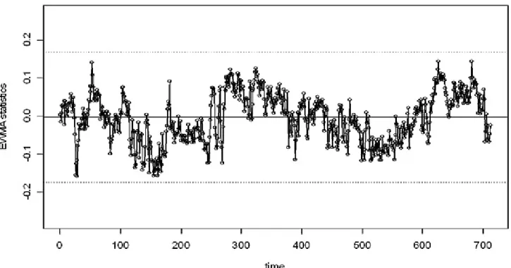
In Phase II, we first obtain the residuals of the 712 data from 2001 to 2002 by fitting Equation (3). The EWMA residual control limits constructed in Phase II is applied to these residuals as shown in Figure 1.
Figure 1. EWMA chart for the residuals of Nantsz’s ln(PM10) data in Phase II using ARFIMA model.
Figure 1 indicates that no residual is out of control, which implies that ln(PM10) data in Phase II is likely to follow the similar pattern of Phase I. Thus, we may conclude that there is no evidence that the air quality of PM10 at Nantsz in Phase II is different from Phase I. This means that the air quality in Nantsz area has not been improved from 1999 to 2002 period. Further corrective actions need to be done. If the long-term autocorrelations were ignored, then the most commonly used models to fit time series are ARIMA models. In contrast with the ARFIMA model, ARIMA model is compared for assessing the suitability of model selection. It is found that ARIMA(0, 1, 2) model could fit the air quality data of Nantsz from 1999 to 2000. However, the residuals are not normally distributed, thus, with a proper Box-Cox transformation(λ=2) the residuals are normally distributed. Similarly, in Phase I, EWMA control chart is applied to these transformed residuals.
After deleting the only out-of-control point, the air quality data are modeled again. The appropriate model can be written as Equation (4).
(1-B) ln(PM10t)=-.0003+(1-0.4031B-0.2883B2) ε
t. (4)
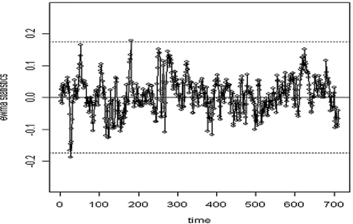
In Phase II, we use Equation (4) to fit ln(PM10) of Nantsz collected between 2001 to 2002. Despite of the fact that residuals could not been transformed to be normally distributed with Box-Cox method in this Phase, EWMA control charts are applied to monitor the residuals without transformation.
Figure 2 indicates that there are two points out of control and its pattern is different from Figure 1. This Nantsz example demonstrates that the ARFIMA model is more appropriate than ARIMA model. False 3 of 4
Research Express@NCKU - Articles Digest
alarms would occur if one selects a wrong ARIMA model instead of using ARFIMA model. In addition, if the diagnosis of residuals have been performed cautiously, it will be found that the ARIMA model does not fit the data because of the residuals have non-constant variance and the autocorrelation function (ACF) of ARIMA model does not resemble the one of ln(PM10) data. The ACF is noticeably important and should be calculated to a very large lag to help us identify the long-memory property. In short, the model fitting in the Phase I should be performed very carefully to avoid the incorrect selection of models, which may lead to false alarms in Phase II.
Figure 2. EWMA chart for the residuals of Nantsz’s ln(PM10) data in Phase II using ARIMA model.
In this paper, control charts using ARFIMA model are proposed to monitor long-memory air quality data. A proper use of control charts can help us understand whether the underlying long-memory air quality model has changed. The proposed procedures of applying ARFIMA models to monitor air quality data can also be used for monitoring other long-memory environmental data. Through the empirical example of air quality of southern Taiwan, we have demonstrated that control charts using ARFIMA models are more appropriate than control charts using ARIMA models in monitoring long-memory air quality data. When monitoring data with autocorrelation, the meaning of “out-of-control” indicates not only the residuals of processes may deviate from what are assumed, but also the underlying model of the process might be changed. The above research findings can be served as a useful reference for setting up an on-line analyzer to monitor the quality change of the environment, so a timely corrective action can be made accordingly.