於無線資料中心啟用一致性網路更新

(1)

國立臺灣大學電機資訊學院資訊工程學系碩士論文

Department of Computer Science and Information Engineering College of Electrical Engineering and Computer Science

National Taiwan University Master Thesis

於無線資料中心啟用一致性網路更新 Enabling Consistent Network Update in

Wireless Data Center

陳冠宇 Kuan-Yu Chen

指導教授：逄愛君博士 Advisor: Ai-Chun Pang, Ph.D.

中華民國 105 年 6 月

June, 2016

(2)

(3)

中文摘要

軟體定義網路 (SDN) 在一致性網路更新機制的可靠度與彈性上帶來新的機會，使得更新過程與底層路由協議無關。隨著無線傳輸技術的進步，越來越多的企業將無線天線佈署在他們的無線資料中心裡。然而，盡我們所知，目前沒有任何的解決方案有將無線干擾考慮進一致性網路更新的模型設計中。當網路資源匱乏時，資源競爭的現象將可能發生，延長整體更新完成的時間。在本篇論文中，用來處理無線干擾的無線資源依賴模型先被提出。接著，為了減緩資源競爭的現象，

一個啟發式的貪婪解決方案被提出。根據模擬的結果，本論文所提出的方法可以有效得於無線資料中心內完成一致性網路更新。這些結果也透露了在一致性網路更新的過程中解決資源競爭的重要性。

(4)

Abstract

Software-defined networking (SDN) brings new opportunities in design of more reliable and flexible consistent network update mechanisms by mak- ing the update process independent of the underlying routing protocols. With the advance of wireless transmission technology, increasing enterprise has deployed radio antennas into their wireless data center. However, to the best of our knowledge, none of the state-of-the-art solutions consider radio interference into their model design of consistent network update. When the network resource is deficient, the resource competition phenomenon may occur, which prolongs the total update completion time. In this thesis, the wireless resource dependency model is firstly proposed to handle the radio interference. Then, a greedy-heuristic solution is provided to alleviate the resource competition phenomenon. According to the simulation results, the proposed solution can efficiently complete consistent network update in wireless data center. These results also reveal the importance of solving resource competition during consistent network update.

(5)

List of Figures

3.1 Example of node capacity . . . 9

3.2 Network update example 1 . . . 14

3.3 Network update example 2 . . . 14

4.1 Dependency graph for Figure 3.3 . . . 16

4.2 Dependency graph for Figure 3.2 . . . 16

4.3 New dependency graph for Figure 3.2 . . . 17

4.4 Introducing temporary state . . . 18

4.5 Example for competitive graph of flow A (solid line) and flow B (dotted line) . . . 19

4.6 Radio antenna deployment on top of each switch racks . . . 27

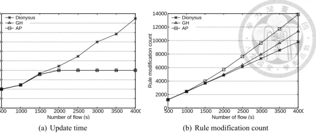
5.1 Update time and rule modification count with different number of flow . . 33

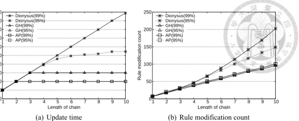
5.2 Update time and rule modification count with various length of Chain . . 35

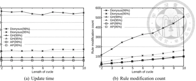
5.3 Update time and rule modification count with various length of Cycle . . 36

(8)

List of Tables

3.1 Notations in problem formulation . . . 10

(9)

Chapter 1 Introduction

Network update is known as changing network state in order to achieve some goals.

More specifically, the network states are commonly referred to forwarding entries, access control lists and many other configurations and status which represent the current settings and state of the network. For example, to conduct traffic load balance, network operator requires to migrate some traffic from heavy-loaded paths to other paths. Specifically, the forwarding entries inside the switches along the affected paths will be updated so as to move traffic toward the new destination.

However, even though the updates are planned carefully in advance, it is naturally difficult to enforce the network to apply these updates correctly, and there still exists some problems during transition from current network state to target network state, such as forwarding loop [1]. The key reason to this phenomenon is the asynchronous update ordering among distributed forwarding devices. Although multiple researches have proposed various solutions to address these problems, these solutions are often too limited to specific protocols, such as BGP and OSPF in routing mechanism of distributed network, and thus are often hard for network operator to apply them into network in an error-free manner.

The emergence of software-defined networking (SDN) brings new opportunities in solving the above mentioned problems. With the logically-centralized controller, SDN decouples the control plane from forwarding plane, which makes the whole networks become programmable, and innovates the network operators to design their applications in a more flexible and fine-grained manner. Leveraging the advantages of SDN, Reitblatt

(10)

et al. [2] provides an abstraction for consistent network update, which aims at preserving well-defined behavior during transition from initial to final state.

Although SDN seems to be a promising architecture in network update, the packets are still forwarded based on individual forwarding rules, which brings challenges in design of the strategy of rule installation. As a result, more and more researches start to focus on different topics on consistent network update in SDN, such as providing guarantees to various consistent properties, or improvement in resource usage and update efficiency.

Unfortunately, current consistent update solutions are still not ready for the future data center networks. In recent years, with the growing demand of data traffic, many links are identified as hotspots, which have much higher probability of being congested compared to other links. Hence, increasing number of industries, including Google [3] and Microsoft [4], begin to apply wireless transmission technology into their data centers to mitigate the hotspot problem. Halperin et al. [4] also show that augmenting wired data centers with wireless links is a promising approach. However, the state-of-the-art consistent update solutions cannot be applied to these wireless data centers directly since these solutions do not consider radio interference.

In addition, scarce of resource during network update may further introduce resource competition and prolong the total update completion time. In existing solutions, given initial and final states, only links in the union set of initial and final paths are considered for traffic migration. Therefore, when these paths are nearly congested, flows can only be moved partially and slowly, despite the fact that some other links may be still left empty.

In this thesis, a wireless data center compatible consistent network update solution is proposed, which not only considers the radio interference model, but also provides a strategy to alleviate the resource competition phenomenon. The contributions of this thesis

(11)

are summarized as follows.

• First, we propose the wireless resource dependency model in solving consistent network update problem.

• In addition, we identify the resource competition problem during consistent network update, and propose an algorithm in constructing competitive graph, which formulates the resource competition relationship between flows.

• Moreover, we propose two methods in picking flows to be migrated to alternative path. The simulation results show the effectiveness of proposed algorithms, which efficiently update the network by alleviating resource competition phenomenon.

• Finally, we propose the idea to find out alternative paths without introducing further resource competition. The details are described in chapter 4.

The rest of this thesis is organized as follows. In chapter 2, related works of state-of- the-art consistent update and radio interference model are provided. The system model and problem formulation are shown in chapter 3. Then, the core idea and solution design are presented in chapter 4. In chapter 5, a complete simulation and result analysis is given.

Finally, we conclude this work in chapter 6.

(12)

Chapter 2 Related Work

The consistency of specific properties during network update has been discussed for a long time in traditional distributed network, but the abstraction of consistent network update was not revealed until the emergence of SDN. Despite the fact that SDN provides a more flexible and fine-grained architecture for consistent update solutions, individual rule installation still brings challenges to the design space. Further, the state-of-the-art solutions cannot be applied to wireless data center directly, since none of them consider the radio interference model. In this chapter, consistent update and radio interference related literatures are investigated.

In the distributed network, researches aim at providing consistency guarantees in specific routing protocols, e.g., BGP, OSPF, during updating current network configurations, such as forwarding entries. For instance, when a topological change occurs, distributed routing algorithm often takes much time to converge on new set of stable routes. Hence, Pei et al. [5] and Siddiqi et al. [6] develop algorithms to cut down the convergence time of BGP and OSPF protocol during update, respectively. On the other hand, modifying network configurations while not lowering the performance or introducing additional is- sues is quite difficult for distributed network routing algorithm. Therefore, the solution proposed by Vanbever et al. [1] and Francois et al. [7] aim at progressively reconfiguring network state without disruption. All these solutions focus on protocol-specific method- ology, which is troublesome for network administrators to systematically integrate them in an error-free manner.

(13)

With the separation of control plane and forwarding plane, SDN provides more flexible and precise architecture, which brings new opportunities to consistent network update problems. Reitblatt et al. [8, 2] is the first to present the abstraction for network update through high-level abstract operations, which allows the programmer to update configurations of entire network without experiencing the painstaking rule installation and switch synchronization procedure. They also introduce two-phase update by first installing the new configurations on internal ports of forwarding devices, and then update the ingress port with new version number to ensure that each packet follows only new or old rules along the paths instead of using mix of old and new rules. The two-phase update guarantees blackhole freedom and loop freedom properties. Blackhole means that a packet entering an SDN switch does not match any rule. After Reitblatt, numerous literatures start involving in the field of consistent update with primary two aspects. One of them aim at providing more consistent properties, such as blackhole and loop freedom [9], way- point enforcement [10] and congestion free update [11]. The other group of researchers focus on improving the current solutions with less resource usage or more efficient way to complete network update [12, 13, 14, 15]. For example, Dionysus [15] leverages the resource dependency model to efficiently schedule the update process. However, none of current researches consider the notion of solving resource competition. As shown in our simulation results, resource competition phenomenon may substantially prolong the total update time and increase the rule modifications, which is absolutely unacceptable for time-sensitive network update.

As the growing trend of wireless data center, many industries start to utilize wireless transmission technology in their data centers, such as Google [3], Microsoft [4], IBM [16].

These researches have shown that wireless transmission is a suitable and promising solu-

(14)

tion which can be used in data center. Unfortunately, none of the current consistent update solutions can be applied to wireless data centers directly, which results from the lack of consideration of radio interference model. Without concerning interference, resource usage and dependency cannot be correctly modelled and thus cannot guarantee some desired consistent properties.

Protocol interference model, proposed by Gupta et al. [17], is one of the most widely adopted model to handle interference; it defines whether two communications are suc- cessful under specific condition. In this model, two wireless transmissions cannot proceed simultaneously if one of the receiver is in the range of interference of the other transmission pair. To reflect the influence on receiving node, some literatures [18] leverage the notion of per-node throughput capacity, which is defined as the throughput that a radio antenna can be used to send and receive, to separate the transmission and interference into different time slice. In the later chapters of this thesis, this notion will be applied in order to achieve resource consistency.

(15)

Chapter 3 System Model and Problem Formulation

3.1 System Model

In a modern data center, some data blocks may be required by many jobs; the nodes which contain these data are called hotspots. These hotspots usually result in link over- subscription and lower down overall performance because large amount of traffic aggregate at specific links. Many researches have proposed various topologies in order to alleviate the hotspot problem, such as Fattree [19], VL2 [20] and BCube [21]. Without loss of generality, we consider Fattree topology in the following discussions. Generally, there are three layers in Fattree topology, including core switches, aggregation switches and Top- of-Rack (ToR) switches. These switches are connected in a cross-layer fashion. More specifically, ToR switches connect to servers in racks and aggregation switches, while core switches connect to aggregation switches and gateways towards public networks.

In SDN, control plane is decoupled from forwarding plane, and each of the switch (forwarding device) forwards packets according to the rules installed by controller. In other words, for each flow path, all the switches along the path are required to have corresponding forwarding rules in order to transfer the packets. In network update problem, given initial and final traffic distribution (each of which consists of some sets of paths of flows), network operator needs to install, modify or delete forwarding rules in order to convert the traffic distribution from initial to final state. An inappropriate ordering of rule installation

(16)

may lead to transient inconsistent state, which may further lower down the performance, e.g. link congestion. Therefore, consistent network update aims at providing legal update orderings of rule operations to maintain consistent properties during update process.

In wireless data centers, 60 GHz transmission technology is often applied due to its outstanding properties, such as high data rate with high radio frequency and short transmission range which fits the dense deployment of switch racks. These antennas are deployed on the top of ToR switches, since the upper space above ToR switches are often kept clear, and wireless transmission can be achieved using directional antenna. However, radio interference is still one of the most challenging problems. In modern data center, owing to space constraints, switch racks are often arranged in a dense fashion. Hence, although high path loss can reduce the influence on radio interference, how to efficiently utilize radio resource remains an important issue.

We use protocol interference model along with node capacity to handle radio interference. Conceptually, if the receiving node of a transmission is in the interference range of another transmission, these two transmissions must be scheduled at separate fraction of time. To realize this notion, we denote node capacity for each radio antenna as how much bandwidth this antenna can support to send and receive with each other. An illustrative example is shown in Figure 3.1. There are two wireless transmissions s₁− d1and s₂− d2

with data rate 300 Mbps and 400 Mbps, respectively. Since node d₁is in the interference range of s₂ − d2, d₁ must receive data at different fraction of time to avoid being inter- fered by s₂− d2. Assume that the maximum node capacity is 1 Gbps for each node. The remaining node capacity on s₁, d₁, s₂, d₂are 700, 300, 600, 600 Mbps, respectively.

(17)

Figure 3.1: Example of node capacity

3.2 Problem Formulation

In this section, some mathematical notations are provided to formulate the consistent network update problem in wireless data center network. These notations are listed in table 3.1 for reference.

A data center can be modelled as a direct graph G = (V, E), where V denotes the set of switches and E denotes the set of links. The link set E is composed of two subsets, including wired links Ewiredand wireless links Ewireless. More specifically, E = Ewired∪ E_wireless and E_wired ∩ Ewireless = ϕ. If there exists a directed link from switch x to y, where x, y∈ V , then there exists an element exy ∈ {Ewired∪ Ewireless}.

Assume that each exy has a corresponding maximum link capacity Lxy. The total traffic passing through link e_xy cannot exceed the maximum capacity L_xy. Recall that radio antennas are only deployed on the top of ToR switches, so that only a subset of switches Vw ⊂ V are equipped with radio antenna. According to the node capacity notion in protocol interference model, we define a maximum wireless transmission capacity W_x for each ToR switch x ∈ Vw. Similarly, the total traffic used to send, receive or being interfered on x cannot exceed the maximum capacity Wx.

In consistent network update problem, initial state and final state are given as require-

(18)

Notation Meaning F Set of flows

G Network graph comprise of (V, E) V Set of switches

V_w Set of ToR switches where V_w ⊂ V

E Set of wired and wireless links where E = E_wired∪ Ewireless

E_wired Set of wired links E_wireless Set of wireless links

e_xy An directed edge from switch x to y L_xy Maximum capacity of link e_xy

Wx Maximum node capacity of radio antenna on switch x S Set of network states

S^k The k^thnetwork state where S^k={R^k, D^k} ∈ S, k ∈ [1, |S|]

D^k The traffic distribution of the k^thstate R^k The rule set of the k^thstate

s_f Source switch of flow f d_f Destination switch of flow f r_f Data rate for flow f

l_f,e^k _xy The traffic load of f on link e_xy of k^thstate

w^k_f,x The traffic load of f on radio antenna of switch x of the k^thstate O^k Set of rule modification operation of the k^thstate

T^k The time to add, modify and delete rules of the k^thstate Table 3.1: Summary of notations

ments. Network operator should convert network state from initial to final incrementally by modifying network configurations, such as forwarding entries in switches, through zero or more intermediate states. Denote S = {S¹, S², ..., S^|S|} as the set of network states from initial to final, where S^k = {R^k, D^k}, k ∈ [1, |S|], denotes the k^th network state.

R^kdenotes the set of forwarding rules inside switches and D^kdenotes traffic distribution on links. Let F be the set of flows in the network. Each flow f ∈ F contains three-tuples (s_f, d_f, r_f), where s_f and d_f denotes the ingress switch and destination switch, and r_f is the data rate for this flow. Note that D^kcan be obtained by forwarding F according to rules R^k, and D^kcan further be divided into D^k_f to represent the traffic distribution occupied by flow f . More concretely, D^k_f ={l^kf,exy|∀exy ∈ {Ewired∪ Ewireless}} ∪ {w^kf,x|∀x ∈ Vw}, where l^k_f,e_xy is the traffic on link exy, while w^k_f,x is the consumed capacity for wireless

(19)

transmission.

Traffic delivery constraint: To ensure blackhole-freedom and loop-freedom property, we define the following constraints to guarantee that all traffic are successfully delivered:

∑

x∈V

l^k_f,e

sf x =∑

x∈V

l^k_f,e

ydf = r_f,

∀esfx, e_yd_f ∈ {Ewired∪ Ewireless}, ∀f ∈ F, ∀S^k ∈ S (3.1)

∑

y∈V

l_f,e^k _yx =∑

z∈V

l^k_f,e_xz,

∀eyx, e_xz ∈ {Ewired∪ Ewireless}, ∀x ∈ V − {sf, d_f}, ∀f ∈ F, ∀S^k ∈ S (3.2)

In equation 3.1, all traffic going out of ingress switch s_f is equal to the traffic received at destination switch d_f. Also, in equation 3.2, all traffic goes into any intermediate switch x must finally goes out with equal amount of traffic. These two equations imply all traffic of flow f at state S^kwill not stay in the network and will not be dropped by any switch.

Resource constraint: There are three kinds of resource constraints, including switch rule set, wired and wireless link capacity, and node capacity for wireless transmission.

Assume R^k_x ∈ R^k denotes the rule set installed at switch x, where ∀x ∈ V , and the maximum rule memory capacity is R_{M ax}, then the following three equations guarantee resource constraints:

|Rx^k| ≤ RM ax,∀x ∈ V, ∀S^k ∈ S (3.3)

∑

f∈F

l^k_f,e_xy ≤ Lexy,∀exy ∈ {Ewired∪ Ewireless}, ∀S^k ∈ S (3.4)

∑

f∈F

w_f,x^k ≤ Wx,∀x ∈ Vw,∀S^k∈ S (3.5)

(20)

Equation 3.3 ensures the rule space constraint, while the remaining two equations state the link or node capacity limitations.

The Efficient Network Update Problem: Given initial state S¹ and final state S^|S|, we want to efficiently convert from S¹ to S^|S| while obeying the above constraints. To convert network state from S^k to S^k+1, we should modify rule set R^k to obtain R^k+1 and D^k+1. In order to consistently modify these rules, we consider the concept of two- phase commitment in [2]. The idea is to firstly install rules with new versions in the downstream network, and then modify ingress switches to apply new version of rules.

Finally, delete the old version unneeded rules. We define rule modification operation O^k = (O^k_add, O^k_mod, O^k_del), meaning the rule operations of add, modify and delete on S^kto change to S^k+1. Define the time to add, modify and delete rules by O^kas T^k = T_add^k +T_mod^k +T_del^k . Note that the time to add, modify and delete rules depends on the finish time of the last updated switch. Take operation of adding rules as an example, let T_x,add^k be the time to add rules at switch x, and if in the k^th state there is no rule addition at switch x, then T_x,add^k will be zero. Then T_add^k = max(T_x,add^k ),∀x ∈ V . Therefore, the objective is to provide these modification operations O^kin order to convert from initial state to final state, which minimizes the total update time T . That is,

Minimize T =

|S|−1∑

k=1

T^k. (3.6)

Furthermore, since rule modification operations are non negligible overhead which bring direct pressure on forwarding devices, we also want to reduce the total number of rule modifications during update process. Formally, reducing the number of rule modification

(21)

operations can be regarded as:

Reduce

|S|−1∑

k=1

|O^k|. (3.7)

3.3 Illustrative Example

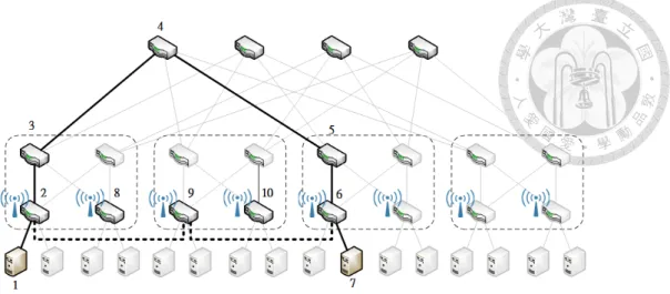
As illustrated in Figure 3.2, assume initially the flow transmits data from host-1 to host-7, passing through switch-2,3,4,5,6. At the final state, it changes to wireless path passing through switch-2,9,6. To complete this update, network operator should firstly install rule on switch-9. Then, modify the rule at ingress switch-2, which changes the flow passing through final path. Finally, network operator can remove the old-version rules on the initial path, including the rules on switch-3,4,5. However, the resource constraints should also be considered, such as wired link capacity and wireless node capacity. Lever- age the notion provided in Dionysus [15], we can create a dependency graph to schedule the update procedure which fulfills the resource constraints. Since Dionysus does not consider wireless transmission and interference, we should modify the model to ensure consistency. We leave the detail design and discussion of modification for dependency model in Chapter 4.

For another example, two flows are required to update from Figure 3.3(a) to Figure 3.3(b), where the solid lines and dotted links are two different flows. Assume both of two flows have traffic volume of 950 unit, and the maximum capacity of all links are 1000 unit. To migrate the first flow from path 1-2-3-4-5 to path 1-2-7-4-5, it requires 950 unit of capacity on link 2-7 and link 7-4, while only 50 unit of capacity remains on each links, which leads to slow update progress since only 50 unit of traffic can be migrated once.

Also, the second flow can only migrate 50 unit of traffic at a time. Hence, for each round,

(22)

Figure 3.2: Network update example 1

(a) Initial distribution (b) Final distribution

Figure 3.3: Network update example 2

both of flows can only migrate 50 unit of traffic and result in 950/50 = 19 rounds to update both of flows to their final distribution. We call this phenomenon resource competition, which can further be classified into Chain and Cycle effect. By Chain, we mean that the remaining capacity of some resource are not enough for one flow to utilize at once, and there exists another flow which will release this resource after its update, forming a Chain of requiring and releasing resource which prolongs the update time since only a portion of resource can be used at once. By Cycle, we mean the last flow in the Chain requires the resource of one of the previous flow in the same Chain, which forms a Cycle.

Both kinds of resource competition will substantially degrade the performance of network update. Hence, to efficiently update the network, we should identify and solve the resource competition phenomenon.

(23)

Chapter 4 Efficient Consistent Network Update in Wireless Data Center

4.1 Wireless Dependency Model

To consistently update the network without violating resource capacity limitations, various literatures have proposed their mechanisms, such as modelling resource capacity as constraints and solve the problem using linear or integer programming tool [11]. How- ever, as shown in [15], such update plan is not adaptive to the actual network update status, and may prolong the total update progress with different update speed of each forwarding switch. Therefore, some researches leverage the update dependency model to dynamically schedule updates according to not only the current network status but also the operation and resource dependencies.

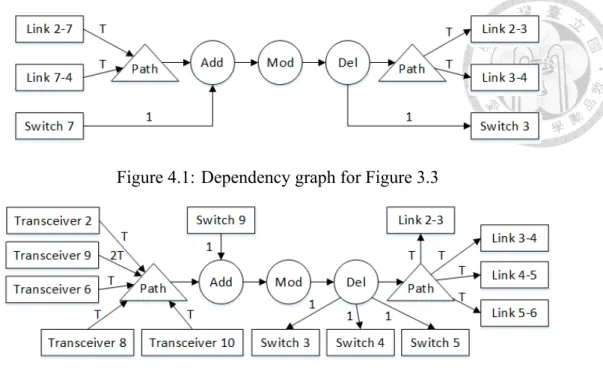
In this thesis, we extend the dependency model in Dionysus with consideration of radio interference model. As stated in Dionysus, there are three kinds of nodes in the dependency graph, including resource, operation and path nodes. For each flow, we can create the operation and resource dependencies according to the difference between their initial traffic distribution and final one. Take the flow with solid line in Figure 3.3 for example, we can construct the dependency graph shown in Figure 4.1, assuming the traffic volume for this flow is T . After creating all dependency links for all flows, we then

(24)

Figure 4.1: Dependency graph for Figure 3.3

Figure 4.2: Dependency graph for Figure 3.2

schedule update according to these dependencies.

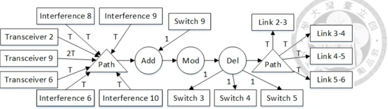
As stated previously, we use protocol interference model along with node capacity to tackle with wireless transmission and interference. Conceptually, a new kind of resource node called transceiver node is introduced to represent the capacity used to transmit, re- ceive and being interfered by a radio antenna. Applying to the dependency model, when- ever a flow requires to transmit from antenna A to antenna B, the capacity on transceiver node A and B are reduced by the traffic volume of this flow. Furthermore, the capacity C of all antennas which is in the interference range from A to B are also deducted by the traffic volume. The remaining capacity on each of C implies they can only communicate with others with different fraction of time. For example, in the Figure 3.2, a flow with initial state as solid line and final state as dotted line will have a dependency graph in Figure 4.2, assuming the traffic volume is T .

However, such modelling is not accurate enough. According to the radio interference model, interference only affects on the receiving nodes, rather than both senders and re- ceivers. For instance, if A is sending data to B and both A and B are in the interference

(25)

Figure 4.3: New dependency graph for Figure 3.2

range of another wireless transmission from C to D, then only B will be interfered and A can still transmit data with the same fraction of time during transmission from C to D.

Hence, instead of only one transceiver node, we propose that one antenna should have two kinds of node capacity, one is transceiver node, and the other is interference node.

For transceiver node, both sending and receiving data will cost capacity. For interference node, both receiving and being interfered will cost capacity. The new dependency graph for Figure 3.2 is shown in Figure 4.3. Note that in the aspect of implementation, if an in- terference node is releasing 50 and requiring 80 of capacity from initial state to final state, then the resulting dependency graph will only have a link for requiring this interference node with capacity of 30 instead of two links requiring 80 and releasing 50.

4.2 Efficient Network Update Problem

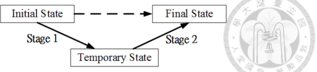
As we can see in the second example in chapter 3, when the network resource is deficient, only small portion of traffic can be migrated at a time and may result in long update time and huge amount of rule modifications. Observing that the resource limitation results from the natural update requirement for each flow from their initial state to final state, the idea to solve this problem is to introduce another temporary intermediate network state.

That is, the update progress will be divided into two stages. In the first stage, instead of

(26)

Figure 4.4: Introducing temporary state

having flow compete on specific limited resource, we migrate some of flows to alternative paths, while the remaining ones just follow the original update plan. In the second stage, we then migrate these flows from alternative paths to their original final paths. This notion is presented in Figure 4.4. Although we increase one stage, if we can guarantee that in both two stages, no resource competition occurs, then the total update time will be effectively reduced. Nevertheless, how to detect resource competition problem, which flows require alternative path, and how to pick up alternative paths remains questions. In the following paragraphs, we divide our method in finding temporary network state into three phases, and show how to efficiently update the network while consuming as least additional resource as possible.

4.2.1 Phase I - Detection of Resource Competition

In order to identify whether the resource competition exists during network update, we firstly create a graph called competitive graph, which reflects the competition relationship between flows. In this graph, nodes are flows, and edges are the competitive relationship between flows. More specifically, an edge exists from flow A to flow B if there exists at least one resource r such that:

a Flow A is requiring r.

b Among all flows requiring r including flow A, the total amount of traffic demand of requiring r exceeds the available capacity of r.

(27)

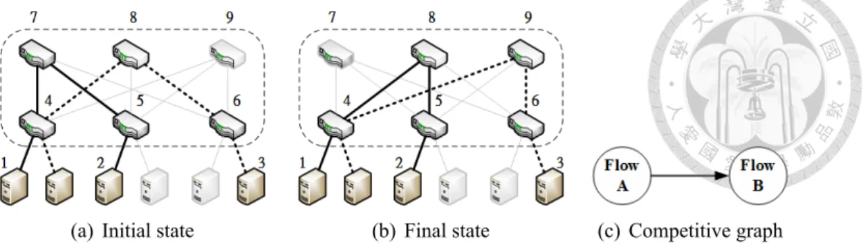
(a) Initial state (b) Final state (c) Competitive graph

Figure 4.5: Example for competitive graph of flow A (solid line) and flow B (dotted line) c Flow B is releasing r.

For requiring resource, we mean that a flow from its initial state to final state, the traffic demand on this resource increases. Conversely, if the traffic demand on this resource decreases, we call it releasing resource. Apparently, a. and c. are the natural demand and supply between two flows, while b. implies that at least one flow will not have enough supply during its update from initial state to final state, and thus competes resource with other flows. For example, if Figure 4.5(a) and Figure 4.5(b) are the initial state and final state of two flows A (solid lines) and flow B (dotted lines), and the traffic volume of both flow A and B are T unit while the maximum available capacity is C unit, then the corresponding competitive graph will be like Figure 4.5(c) if C− T < C, since flow A will compete on link 4-8.

The pseudo code of creating competitive graph is shown in algorithm 1. From line 2 to line 7, initial resource of each flows is pre-occupied, while from line 8 to line 15 the requiring resource are also accumulated. From line 16 to 24, if the total traffic demand on each resource exceeds the maximum available traffic, all flows requiring this resource will have an edge connecting to all flows releasing this resource.

Let the average length of initial and final path of each flow be P . Since the resource used by each flow is determined by the length of initial and final paths, we can regard the total resource involved in this update as O(|F | × P ). Therefore, the complexity from line

(28)

1 to line 15 is O(|F | × P ). We further assume the number of flow requiring or releasing some resource res_D which exceeds M aximumCapacity be |Fe|, then the complexity of line 18 and 19 will be O(|Fe|). Hence, the total complexity for algorithm 1 will be O(|F | × P × |Fe|).

Algorithm 1 Constructing Competitive Graph

Input: A set of flows with their initial and final traffic distribution requirements.

Output: Competitive graph G_cp= (V_cp, E_cp)

1: Initialize all resource res with zero demand res_D

2: for each flow f in F do

3: for each resource res used in initial distribution of f do

4: Let v^f_resbe the used traffic volume by f

5: res_D := res_D + v_res^f

6: end for

7: end for

9: Calculate the requiring resource list RQ_f

10: Calculate the releasing resource list RL_f

11: for each requiring resource res in RQ_f do

12: Let v^f_resbe the required traffic volume by f

13: res_D := res_D + v_res^f

14: end for

15: end for

16: for all resource res do

17: if res_D > M aximumCapacity then

18: for each flow f_xcontaining res in RQ_f_x do

19: for each flow fy containing res in RL_f_y do

20: Add an directed edge e_f_x_,f_y in E_cp

21: end for

22: end for

23: end if

24: end for

4.2.2 Phase II - Flow Picking

In this phase, we are going to pick up some flows in the competitve graph, and change the update plan for these flows from “initial path to final path” to “initial path to alternative path” and “alternative path to final path.” In the competitive graph, we call the path with length longer than or equal to 1 as Chain, and if the last node in Chain connects to another

(29)

node in the same Chain, then we call it Cycle. Obviously, if there does not exist any Chain in the graph, then no resource competition exists. Hence, the problem becomes to “how to pick up some of the flows which breaks all existing Chains and Cycles,” and this can be regarded as the classical vertex cover problem.

A naïve method (called all-picked method) to resolve the resource competition be- tween flows is to break all the Chains in the graph by picking all nodes involving in any Chain. That is, for each flow involves in any of Chain in the graph, we find out an alterna- tive path for it, and these flows will no longer compete with the original requiring resource.

For the remaining flows that do not involve in any Chain, they follow the original update plan. However, on the one hand, though such picking method seems effective in resolving competitions, it may bring huge overhead to forwarding devices. On the other hand, if we try to break all Chains by picking up the minimum number of flows, then it becomes to the classical NP-Complete problem: “Minimum Vertex Cover,” where we cannot find out a feasible solution in polynomial time unless P=NP.

We propose our greedy-heuristic method by improving the deficiency of picking all flows, and pick up as least nodes as possible. To improve the all-picked method, one observation is that the actual resource competition on specific resource may not involve in all flows requiring it. For example, imagine 99 flows requiring 1 unit and 1 flow requiring 100 unit. If the total available capacity for this resource is 100, then all 100 flows will have an edge from themselves to all flows releasing it. Apparently, we can keep 99 flows following their original plan and find out an alternative path for the flow requiring 100 unit of resource, which saves 99 alternative paths. Hence, we iteratively check if each flow has enough resource individually. If so, then we reserve this flow as “Not_picked”

by removing all its incident edges. To pick as least nodes as possible from the remaining

(30)

nodes, we firstly virtually pick up all flows involving in Chain. Then, starting from the least degree of node, we incrementally try to release the virtually picked nodes, by checking if all its neighboring nodes are already picked. If so, we can ensure that all links connected to this nodes are already covered and hence release this node. The insight is that if we successfully release a node, then all its neighbors will absolutely be picked. Hence, the less degree a node is, the less neighbors will be picked to release one node.

The pseudo code of this method is shown in algorithm 2. From line 2 to line 7, initial resource usage of each flows are occupied. From line 8 to line 27, we try to remove some links connected by some flows by firstly checking whether all requiring resource of such flow are enough. By removing these links, the subsequent procedure will regard these flows as “not picked”. From line 28 to line 50, we initially pick up all flows with at least one incident link. Then, starting from the smallest degree of flows, we greedily “un-pick”

these flows if all its neighbors are picked.

As mentioned previously, the number of resource involved in this update are O(|F | × P ). Hence, from line 1 to line 17, the complexity will be O(|F | × P ). Since in Gcp, the number of neighbors for each flow will be at most O(|Fe|), the complexity from line 18 to line 27 will be O(|F | × |Fe|). In line 28, sorting |F | flows in Gcp costs O(|F |lg|F |).

The complexity of remaining lines will be O(|F | × |Fe|), and the total complexity for algorithm 2 will be O(|F | × (P + lg|F | + |Fe|)).

4.2.3 Phase III - Alternative Path

Without Introducing New Chain, Cycle and Deadlock

After deciding which set of flows to pick, we are required to find out alternative paths for these flows. Since we leverage the additional resource, such as switch memory, wired

(31)

Algorithm 2 Greedy Heuristic Picking Method Input: Competitive graph G_cp= (V_cp, E_cp)

Output: A competitive graph with each node marked P icked or N ot_picked

1: Initialize all resource res with zero demand res_D

3: for each resource res used in initial distribution of f do

4: Let v^f_resbe the used traffic volume by f

5: res_D := res_D + v_res^f

6: end for

7: end for

9: enough := T RU E

10: Calculate the requiring resource list RQ_f

11: for each res∈ RQf do

13: if resD + v_res^f > M AXIM U M _CAP ACIT Y then

14: enough := F ALSE

15: break

16: end if

17: end for

18: if enough = T RU E then

19: for each ef,fx in Ecpdo

20: Remove e_f,f_x and e_f_x_,f in E_cp

21: end for

22: for each res∈ RQf do

24: res_D := res_D + v_res^f

25: end for

26: end if

27: end for

28: Sort all nodes in Gcp with non-decreasing degree

29: for all nodes f in F do

30: if degree(f ) > 0 then

31: M ark[f ] := P icked

32: else

33: M ark[f ] := N ot_picked

34: end if

35: end for

36: // The remaining part of this algorithm is on the next page

(32)

37: for each node f in G_cp do

38: if degree(f ) > 0 then

39: all_picked := T RU E

40: for each neighboring node f_nof f do

41: if M ark[f ] = N ot_picked then

42: all_picked := F ALSE

43: break

44: end if

45: end for

46: if all_picked = T RU E then

47: M ark[f ] := N ot_picked

48: end if

49: end if

50: end for

link capacity and radio antennas, we must ensure that requiring these resource will not introduce new Chains, Cycles and Deadlocks at final state. As mentioned previously, we can partition the update progress into two stages, one is from initial to temporary state, where some of flows are migrated to alternative paths and the remains follow the original plan. The other is from temporary to final state, where the flows on alternative paths are finally migrated to their original final paths. Conceptually, if we can guarantee that in both stages, no additional Chain, Cycle and Deadlock are introduced, then there will be no Chain, Cycle and Deadlock during the whole update progress. More specifically, for each flows required to be migrated to alternative paths, the requiring resource from initial path to alternative path must not introduce new resource competition in first stage.

Similarly, these flows must not introduce new resource competition when migrating from alternative path to final path in the second stage.

Since we firstly update the network from initial state to temporary state, and then from temporary state to final state, we can treat the resource usage of two stages separately.

That is, each stage has a resource copy of the network. In the first stage, we can pre- occupy the following resource. a. the initial traffic distribution on initial paths of all flows. b. the final traffic distribution on final paths of the un-picked flows. By b., all the

(33)

requiring traffic by the un-picked flows are occupied in advance, and hence no matter what resource will be leveraged later, no additional resource competition will occur. Similarly, in the second stage, we can pre-occupy the final traffic distribution of all flows to prevent us from using the resource on final distribution, which can avoid further deadlock since no resource will be released on final state. Hence, for any alternative path of any flow, if the requiring resource from initial path to alternative path do not exceed the available resource on first stage, and the requiring resource from alternative path to final path do not exceed the available resource on second stage, then we can guarantee that non of Chain, Cycle or Deadlock will occur during update. Note that in the first stage, if there are overlapping resource between initial path and final path of a flow, then such resource will be occupied only once. One may notice that in the first stage, sometimes occupying both initial and final distribution may exceed the total available capacity of some resource. This do not affect the correctness since the requiring resource for alternative path should regard this as “out of resource.”

In wireless data center, since wireless paths are more likely to have fewer hops than wired paths, which implies fewer switch memory consumption for forwarding rules, we always try to find out wireless path first. If wireless path cannot fulfill the resource constraints, including both mentioned in chapter 3 and previous paragraphs, then wired paths are tried subsequently. For any kind of alternative path, the less hops are required, the less network resource are consumed. Hence, we always apply shortest path in searching alternative paths. The details of searching wired or wireless paths are shown in the following subsections.

(34)

Wired Alternative Path

In Fattree topology, searching paths with shortest route can be classified into three cases according to the position of source and destination hosts. First of all, if source and destination share the same ToR switch, then only one path fits, which is from source to ToR switch and then from ToR switch to destination. Otherwise, if the source and destination share the same pod, then there are^k₂ paths can be chosen, since there are^k₂ candidate aggre- gate switches can be used, assuming k is the total number of pods. Hence, each of these paths will consists of source, T oR₁, Aggregate, T oR₂ and destination switch. Finally, if source and destination are in different pod, then there will be ^k₄² possible paths, since each of ^k₂ aggregate switch will have ^k₂ candidate core switches can be chosen from. The resulting path will consists of source, T oR₁, Aggr₁, Core, Aggr₂, T oR₂ and destination switch.

Whenever there are more than one candidate switch, we randomly pick up one with uniform distribution. In doing so, we expect that the traffic distribution on each of these paths will also uniformly distributed, preventing congestion on specific links. If the picked up path does not fulfill the resource constraints, then we will pick up the next possible paths randomly, and continue until one feasible path is found or all candidates are enumerated.

For all cases, finding out a feasible wired paths will have the worst case complexity of O(k²), since there are at most ^k₄² candidates when source and destintion are in different pod.

Wireless Alternative Path

In modern wireless data centers, there are often hundreds of ToR switches, which means that there will be hundreds of radio antennas. In this thesis, we reference to the

(35)

Figure 4.6: Radio antenna deployment on top of each switch racks

switch rack deployment provided by Microsoft [4]. As shown in figure 4.6, on the top of each rack, a 60 GHz radio antenna is deployed, which can be used to send and receive data with another radio antenna.

From source to destination, a wireless path may consist of one or more hops. There are too many choices of wireless paths can be selected, and it is infeasible to search alternative shortest paths during network update, since it may waste too much time in exhaustively try- ing all possible paths. As a result, we pre-process and preserve one wireless shortest path for each pair of source and destination before update. During update, the pre-processed paths are examined and checked if it can fulfill all constraints mentioned above. Note that since we only preserve one wireless path for one pair of source and destination, if such path does not fulfill the resource constraint, then we will regard it as “path not found”.

In searching the wireless shortest paths, if there exists multiple possible equal-length paths, then the one with least total number of interfered switches are chosen. By total number of interfered switches, we mean that along the path, the total number of switches that is in the interference range for each hop. The reason for picking such paths is to reduce the total number of resource consumed. Using Shortest Path Faster Algorithm (SPFA), the complexity of searching single-source wireless shortest paths will be O(cE), where E is the number of wireless edges and c is a number smaller than 3 in average case.

(36)

Therefore, searching for all pair wireless shortest path will be O(cV E) with V different source switch.

The pseudo code for searching single-source wireless path is shown in algorithm 3.

From line 1 to line 5, all relevant variables are initialized, where dis and itf denote the minimum distance and minimum total number of interfered switches start from some switch S_x, while pre is used to record the previous hop in the path. From line 6 to line 30, a modified SP F A algorithm is presented. For each switch popped out from queue (line 10-11), all neighbors are examined (line 12) to update the minimum distance and minimum interference count. Line 13 to line 19 means the case if shorter distance can be reached, while line 20 to line 28 check if smaller interfered switch count can be achieved when the distance is equal to current minimum one. From line 31 to line 37, the optimal alternative paths are retrieved for all possible destinations, and store to the path list P ath.

Since in the wireless data center, all ToR switches can be reached using radio antennas, which means the graph is connected, there is no need to check if destination switch S_dst is reached (P re[S_dst]̸= −1) or not.

The complexity of checking whether one path fits the constraints depends on the length of this path, which is O(P ). For wireless paths, since we pre-process and reserve one path for each pair of source and destination, the complexity of checking will be O(|Fe|×P ). For wired paths, at most^k₄² paths will be checked, resulting in complexity of O(|Fe|×k²×P ).

According to the update process of dependency model, the complexity of updating all flows will be O(I × |F | × (P + lg|F |)), where I is the number of update iterations.

The condition that our computing complexity is lower than update process will be O(I) >

O(^P|F |lg|F |+|F |×P^×|F^e^{|×(|F |+k}²⁾). This condition can be easily fulfilled when resource is scarce.

(37)

Algorithm 3 Single-source Wireless Alternative Path Input: Network Topology; Source switch Ssrc

Output: Wireless alternative paths list P ath[Ssrc][S_dst] for all S_dst

1: for each S_xin all switches do

2: dis[Sx] := IN F

3: itf [S_x] := IN F

4: pre[S_x] :=−1

5: end for

6: dis[S_src] := 0

7: itf [S_src] := 0

8: Push Ssrc into Q

9: while Q is not empty do

10: S_now := Q.f ront()

11: Q.pop()

12: for each enow,nxtin E_wirelessdo

13: if dis[S_now] + 1 < dis[S_nxt] then

14: dis[Snxt] := dis[Snow] + 1

15: itf [S_nxt] := itf [S_now] + itf List[S_now][S_nxt].size()

16: pre[S_nxt] := S_now

17: if Snxt is not in Q then

18: Push S_nxtinto Q

19: end if

20: else if dis[Snow] + 1 = dis[Snxt] then

21: if itf [Snow] + itf List[S_now][S_nxt].size() < itf [S_nxt] then

22: itf [S_nxt] := itf [S_now] + itf List[S_now][S_nxt].size()

23: pre[Snxt] := Snow

24: if Snxt is not in Q then

25: Push S_nxtinto Q

26: end if

27: end if

28: end if

29: end for

30: end while

31: for each S_dstin all switches except S_src do

32: Snow := Sdst

33: while Snow ̸= −1 do

34: Push S_now into front of P ath[S_src][S_dst] list

35: S_now := pre[S_now]

36: end while

37: end for

(38)

Chapter 5 Performance Evaluation

5.1 Simulation Environment

5.1.1 Simulation Settings

In this thesis, a large scale simulation based on wireless data center with Fattree topology is developed. Totally, there are 500 switches with a three-layer architecture, including 100 core switches, 200 aggregate switches and 200 ToR switches. We consider the similar switch rack deployment provided by Microsoft, and on the top of each switch racks, one 60GHz radio antenna is placed, just as shown in Figure 4.6. We assume that the maximum available link capacity of wired links and node capacity of wireless APs are 1 Gbps when there is no transmission. Since these radio antennas are statically placed, the transmission and interference range can be easily derived. The switch memory, TCAM, which is used to store the forwarding rules given by controller, has available capacity of 1500 rule slots by default. As for the time for rule modification, we set modifying rule as 10 ms and installing/deleting rules as 5 ms each according to the measurement provided by [15].

During update, each round consists of rule install, modify and delete, and thus the average total update time for one round is set as 20 ms in this thesis.

(39)

5.1.2 Scenario Design

To reflect the influence on resource competition, three different scenarios are designed.

The first one is used to test the performance on normal case, where the source and destination of each flow are randomly generated. The last two are to simulate the traffic migration when resource are deficient, one for Chain and the other for Cycle. That is, on these nearly congested links, we migrate the flows from one link to another, forming a Chain or Cycle with different lengths ranging from 1 to 10. In the all three cases, the data rate for each flow are generated according to the real traffic measurement [22]. The details of design of these three scenarios are shown in the following paragraphs.

Random Source Destination Pair

In this case, each of flows are generated by randomly picking source and destination pair. Although randomly generated, Chain amd Cycle may still exist, while the formula- tion of these effect occur naturally. In this thesis, we set the number of generated flows ranging from 500 to 4000.

Heavy Loaded Chain and Cycle

To embody the resource competition effect on specific links, we firstly choose L links in the network. In order to simulate the nearly congested situation, for each of these chosen links, we continuously generate flows passing through it until 99% of capacity on these L links are occupied. If some flows cannot pass through one link before reaching 99%

of capacity, then we randomly pick a pair of source and destination, and make the flow become background traffic. Once all these L links are done, then for each of L− 1 links from the first to the L−1^thone, we pick up one of flow with highest data rate and migrate

(40)

it to the next links, forming a Chain. For generating Cycle, we further migrate the flow with highest data rate in the last link to the first one. In this thesis, we set the length of L from 1 to 10. For comparison, we also generate the case of occupying 95% of capacity, instead of 99%.

5.1.3 Methods in Comparison

To compare with the proposed greedy-heuristic algorithm (abbreviated as GH), two additional methods are considered. The first one is the original version of Dionysus, which does not consider the resource competition phenomenon. The second one is the naïve all- picked method (abbreviated as AP ), which picks up all the flows involving in any of Chains, and find out alternative paths for each of them.

5.2 Result Analysis

The simulation results of three different scenarios are shown and discussed. For each of these scenarios, we execute 50 times and calculate the average value for each metric.

In heavy loaded scenarios, solid lines denote the cases of occupying 99% of link capacity, while the dotted lines denote the 95% ones.

5.2.1 Random Source Destination Pair

For the case of random generated source and destination, when the number of flow is below 1500, the network resource is still not exhausted, resulting in few Chains and Cycles. Hence, the performance of AP and GH are just closed to Dionysus. However, when more flows co-exists in the network, increasing Chains and Cycles are generated, which prolongs the update time of Dionysus.