Zhang-McFarlane積雲對流參數化中次網格對流與對流覆蓋比例關係之探討

國立台灣大學理學院大氣科學研究所 碩士論文

Department of Atmospheric Sciences College of Science

National Taiwan University Master Thesis

Zhang-McFarlane 積雲對流參數化中 次網格對流與對流覆蓋比例關係之探討

On the Convective Updraft Fraction Dependency of Sub-grid scale Vertical Transport in

Zhang-McFarlane Convection Parameterization

郭威鎮 Wei-Chen Kuo 指導教授：吳健銘 博士 Adviser: Chien-Ming Wu, Ph.D.

中華民國 106 年 1 月

January 2017

致謝

即使到了要交出論文的前夕，寫下這篇致謝文的心情依然是忐忑不安的。回 想這兩年半以來的研究過程，遇到許多困難和突發狀況，因此越接近終點的此刻，

反而有種如履薄冰的縹緲感。剛進到研究所時，覺得閱讀論文、抓程式碼裡的蟲、

上台報告…等等都是異常困難的事情，有好幾次報告前都還想著要臨陣脫逃(但 還是沒逃，因為既可恥又沒用)。這些事情不像教科書裡一樣，有那麼明確的答 案可以提供參考。許多問題都需要靠冷靜、耐心和變通，加上足夠的理解、消化、

再理解、再消化…，反覆幾次之後或許會達到，也或許不會達到預期的目標，但 是在這段迂迴的過程中所累積的經驗，是如同非保守力做功一樣不會走回頭路的。

很感謝老師對科學研究的堅持、對學生的包容和鼓勵，讓我在面對風雨時仍能夠 靜下心來，體悟研究背後的科學，並思考自己的路(還同時修了日文三、韓文一、

二和旁聽了一學期泰文一)。很感謝實驗室的夥伴們提供各種技術上、概念上、

物質上和心靈上的協助，一起吃飯、聊天、抵霸格、看日出，讓我不再只會苦苦 哀求魚吃，還能夠拿著釣竿跟大家一起快樂的覓食。很感謝家人和朋友的體諒和 等待，研究成果出爐的時間似乎比預期的還要長，也幸好等待是有成果的，能夠 讓我無愧於自己對研究目標的想像。回憶很多，寥寥數語難以言表，我想，就讓 它好好的沉澱在腦海裡，等到將來的某一天有興致時再翻開這本書，或許這些畫 面又會一一浮現出來吧！

摘要

全球環流模式在解析度逐漸提升的過程中，所使用的對流積雲參數化也必須 隨之相應的減少其作用，才能在解析度提升至雲解析模式時，自動將參數化之功 能解除。為了發展出整合性參數化方法，Arakawa and Wu (2013) 使用 GATE 個 案在 VVM 當中的模擬，並以不同次網域大小作平均，將之視為不同解析度下的 全球環流模式網格資料，再去分析其中的次網格對流強度隨解析度之關係。他們 提出對流覆蓋率是整合不同解析度模式的適當參數選項，並用此參數推導出整合 性參數化方法，當次網格對流覆蓋率接近網格尺度時，藉由此參數來調降參數化 之強度，避免重複計算。本研究旨在推廣此一參數化方法在不同對流強度之適用 性，及配合現有之積雲參數化來進行整合性參數化試驗。我們所用的個案為對流 強度變化較 GATE 個案多的 DYNAMO 實驗，也將 DYNAMO 實驗依照降水強度 分成四類，並沿用 Arakawa and Wu (2013) 的實驗方法進行分析，結果顯示在 DYNAMO 整體及不同強度降水的次網格對流中，其對流覆蓋率關係是類似的，

因此使用對流覆蓋率作為參數之整合性參數化在不同對流強度下也適用。我們也 首度將整合性參數化結合 Zhang-McFarlane 積雲參數化以及兩種不同的對流垂直 速度參數化方法，並用來計算 DYNAMO 實驗中的次網格對流強度。整合性參數 化結果顯示所得到的對流覆蓋率有偏低且偏離實際對流網格的情形，其主要原因 為診斷之垂直速度過大及積雲參數化對流為垂直發展之限制。在整體參數化對流 強度方面，傳統和整合性之結果差異不大，主要原因為對流覆蓋率過小，而原本 與對流覆蓋率無關係之傳統參數化對流，則藉由此參數化方法調整至較接近雲解 析模式之結果。

關鍵字：對流積雲參數化、整合性參數化、對流覆蓋率關係

Abstract

Statistics of convective updraft fraction (σ) dependence, using the analysis methods in Arakawa and Wu (2013) (AW13), in a 15 days period of time-variant thermodynamic forcing case (DYNAMO), and the offline test of unified parameterization (UP) closure combined with Zhang-McFarlane parameterization scheme (ZM) are presented in this work. The similar result of σ dependence within DYNAMO and GATE (used in AW13), and of the four different strength categories of precipitation in DYNAMO explain that the σ dependence is more appropriate than

resolution dependence for unified-parameterizing multi-phase convection. The UP closure proposed by AW13 uses σ as the tuning parameter to adjust the conventional

parameterized convection, which lacks of consciousness of sub-grid scale convection coverage. The results of inputting DYNAMO forcing into the ZM, combined with UP

and vertical velocity parameterization scheme, which is for diagnosing unknown σ in the closure, shows the underestimation of the σ values and the shift of convective areas

away from the cloud resolving model (CRM) simulation, causing the problem of tuning down the parameterized mass fluxes at incorrect places. This can be improved by revising the closure that decides the place of convection and tuning the in-cloud vertical velocities to a more reasonable scale. The purpose of UP scheme is to adjust the

sub-grid scale convection by regarding its parameterized σ, so even the ensemble average of convection fluxes doesn’t significantly changed after applying UP scheme, the σ dependence of unified parameterized convection fluxes still better fit the σ dependence in the convection of CRM.

Keywords: cumulus convection parameterization, unified parameterization, σ

dependence

Contents

口試委員會審定書……… i

致謝……… ii

中文摘要………..………. iii

Abstract………. iv

1. Introduction………. 1

2. Dependence of sub-grid scale convective updraft in DYNAMO……… 6

3. The derivation of unified parameterization scheme……… 23

3.1 The revision of conventional closure to unified closure……….. 23

3.2 Parameterize σ from boundary convection scheme………. 28

3.3 Combination with Zhang-McFarlane Scheme………. 31

4. Analysis of unified parameterized convection……….. 33

5. Conclusion and future work………... 47

References……… 51

Appendix………... 54

1. Introduction

In the simulation of global weather systems by using general circulation models (GCMs), cumulus convection parameterization schemes are necessarily applied because of the relatively coarser resolutions. The development of numerical computing in these decades gradually increased the resolution of GCMs toward cumulus convection scale. If the resolution of GCMs is high enough for simulating cumulus convection, the parameterization should play no role in the models. As the resolutions converging from GCMs to cloud resolved models (CRMs), which are without parameterizing process of cumulus convection, the conventional parameterization scheme designed for coarser resolutions should do corresponding changes during the down-scaling process of models. Several efforts have been made for unifying cumulus parameterization that automatically adjusts itself across scales (e.g., Fan et al. (2015); Lappen and Randall (2001), Part I, II, III; Liu et al. (2015); Jung and Arakawa (2004)). Arakawa and Wu (2013) (abbreviated as AW13 in the following contents) referred the simulation of Global Atmospheric Research Program (GARP) Atlantic Tropical Experiment (GATE) in 2km-resolving vector vorticity model (VVM, one of the CRMs) as “true” solution to find the appropriate representation of sub-grid scale convection in GCM. The original CRM grids are gathered into different sizes of

square sub-domains (e.g. 4km, 8km, etc.), pretending as the grid cells in GCM. For these GCM-like sub-domains, CRM grid size convections are unable to be resolved, as the role of sub-grid cumulus convection in GCM grids. By analyzing the statistics of convection in sub-domains crossing different sub-domain sizes, AW13 claimed that convective updraft coverage ratio (σ) dependence of sub-grid size convection is more appropriate than resolution dependence since the ratio of sub-grid convection and total convection strength can vary largely in the same resolution but rather consistent in the same σ (fig. 9 in AW13). In AW13’s experiment, a 24-hr constant forcing of GATE is used to trigger the convection in VVM, resulting in the relatively strong precipitation series during the most of the simulation period (red line in fig. 1).

Further investigation in σ dependence of different convection phases is needed since the statistics of sub-grid scale convection can vary largely within suppressed and active phases. Xiao et al. (2015) also pointed out that the resolution dependence of sub-grid scale convection output from convection parameterization (Zhang-McFarlane) is sensitive to the strength of convection.

To better interpret the σ dependence of sub-grid scale convection under multiple conditions, we run through the experiment methods that mentioned in section 2 of AW13, but choose Dynamics of the Madden Julian Oscillation experiment

(DYNAMO) from 15^th October to 30^th October, 2011 as our analysis data instead. From

the time series of VVM-simulated domain-averaged precipitation in GATE (red line) and DYNAMO (blue line), we can figure out that DYNAMO has the more time-variant thermodynamic forcing during 15 days of simulation, while the forcing in GATE remains relatively strong in a much shorter period (24 hours). The relatively weaker and stronger convection phase may reveal different statistics on σ dependence of sub-grid scale convection, so we also divide the simulated data of DYNAMO into four groups according to their precipitation rate, and re-operate the analysis of σ dependence. The details of analysis methods and results are shown in section 2.

Figure 1 Space-averaged precipitation (mm/hr) of 24-hour simulation using GATE constant

forcing (red line) and of 15-day simulation using DYNAMO time-variant forcing (blue line)

both in VVM, and the precipitation (mm/hr) from Zhang-McFarlane parameterization output

using whole domain-averaged DYNAMO forcing (yellow line).

In the following contents, we try to put the unified parameterizing processes more forward to application in modeling simulation. AW13 used the σ dependence of sub-grid scale convection as the tuning parameter, and also eliminate the assumption of “σ << 1” in the unified parameterization (UP) closure. Most conventional cumulus parameterizations assume that the thermodynamic variables of GCM grid-scale can be referred to those in the environment of cumulus convection, implying that the coverage of convective updrafts are much smaller than the grid sizes (AW13). This assumption confronts strict challenges as the resolution of GCMs converges to convection scale, causing the convection to become closer to grid-scale in some convective areas. Moreover, the conventional parameterizations only parameterize the values of convection mass fluxes, which is the product of σ and updraft velocities.

Even if the assumption of “σ << 1” is eliminated, there still need more tools to separate σ and updraft velocities. We use Zhang-McFarlane (ZM) parameterization

scheme combined with UP closure and the additional vertical velocity parameterization schemes, including ECMWF (2010) and Kim and Kang (2011), to help us parameterize the in-cloud vertical velocities and derive σ. ZM scheme is the cumulus convection parameterization scheme used in CAM that developed by NCAR, which is one of the major model for climate simulation, and the parameterized convection can severely affect the long-term energy budget. In the standard operation procedures of cumulus parameterization, the parameterized convection fluxes are added back to the directly simulated variables and then be integrated to the next time steps, which is called online approach. This approach will also integrate the parameterized variables nonlinearly through the simulation, making it much more difficult to track the sources of biases in UP closure, so we choose the offline approach through the whole simulation, which means that the parameterized fluxes derived from the cumulus parameterization scheme are only for analysis after outputting, without adding back to the directly simulated convection fluxes. The thermodynamic forcing used to trigger ZM scheme are from the DYNAMO case that has been averaged by different sub-domain sizes, regarded as grid cells in GCM. Before running unified-ZM scheme and analyzing the results, we use the conventional ZM scheme to simulate the time series of whole domain precipitation rate, which is shown as yellow line in fig. 1

and much smaller than the simulation in CRM (blue line). The details of deriving UP closure in AW13 and the vertical velocities parameterization schemes used in our work are shown in section 3, and the results of applying ZM scheme with UP closure are shown in section 4.

2. Dependence of sub-grid scale convective updraft in DYNAMO

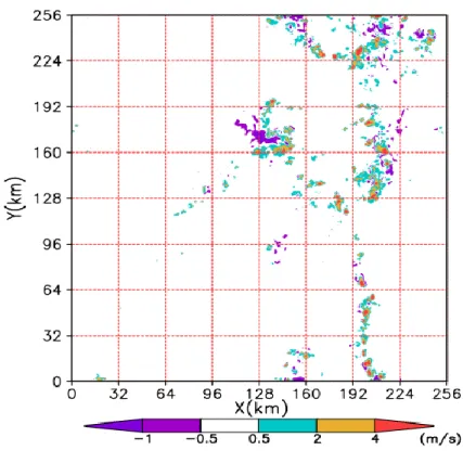
The simulation of DYNAMO active phase (within 15 days; from 2011/10/15 to 2011/10/29) in this study is simulated by the Vector Vorticity Model (VVM), using 256 km x 256 km horizontal domain with 1km grid size, and 34 vertical stretching grids from 100m at lower boundary to 1000m at about 19km height. To realize the statistics of sub-grid scale convection fluxes in different GCM-like grid sizes, we divide the original 256km x 256km domain into different sizes of sub-domain (1, 2, 4, 8, 16, 32, 64, 128, 256km), regarding each sub-domain as a grid cell in GCM, and evaluate the sub-grid scale convection strength. Fig. 2 is the example of whole domain divided by 32 km size of sub-domains.

Figure 2 Snapshot of whole horizontal domain at 500^th time steps, 3km height. Shaded color

represents the vertical velocity, and red dot line grids are 32 km sub-domain grids. Only the

sub-domains with any convective updraft grid (w ≥ 0.5m/s) are chosen as samples to calculate

< 𝑤ℎ̅̅̅̅ > and < 𝑤̅̅̅̅̅̅ >. ^′ℎ^′

We use the definition following AW13: 𝑤̅, ℎ̅ are the averaged vertical velocity and moist static energy of CRM grids in a single sub-domain grid, which can be

regarded as GCM-like grids, and 𝑤^′, ℎ^′ are the deviation of CRM grid values from 𝑤̅, ℎ̅, respectively. For the sub-domain size grid cells, 𝑤̅, ℎ̅ are resolvable while 𝑤^′, ℎ^′

are the unresolvable variables. The sub-grid scale vertical eddy fluxes of moist static

energy (MSE) can be written as 𝑤̅̅̅̅̅̅ where the overbar represents the sub-domain ^′ℎ^′ average values. Since the parameterized convection is only triggered in the grid points that reach a particular threshold, 𝑤̅̅̅̅̅̅ of sub-domains with any grid point that have ^′ℎ^′ vertical velocity larger than or equal to 0.5m/s, are chosen as the convective ensemble members. The ensemble-averaged 𝑤̅̅̅̅̅̅ is denoted as < 𝑤^′ℎ^′ ̅̅̅̅̅̅ >, which represents ^′ℎ^′ the convection fluxes that need to be parameterized in the ensemble members.

The degree of parameterization that is required for sub-grid scale convection in

sub-domains can be evaluated by the ratio between vertical eddy fluxes and total fluxes of MSE (< 𝑤̅̅̅̅̅̅ >/< 𝑤ℎ^′ℎ^′ ̅̅̅̅ >) as shown in fig. 3 for a selected level at 3km height,

which is close to the layer of largest < 𝑤̅̅̅̅̅̅ >. The results show that when the ^′ℎ^′ sub-domain sizes are much larger than the scale of cumulus convection, the sub-grid scale convections dominate the total convection strength. The degree of required parameterization dramatically decreases as the sub-domain sizes become closer to 1km since sub-grid scale convection is more resolvable in finer resolutions. If there is an ideal unified convection parameterization, it should pick up the main sources of convection at conventional GCM resolutions and ease its task as the resolution gradually reaches to cumulus convection scales, as the results of AW13. The relations between total and eddy convection fluxes at other heights also show the similar results

as 3km height (fig. 4 and fig. 5).

Figure 3 < 𝑤̅̅̅̅̅̅ > and < 𝑤ℎ^′ℎ^′ ̅̅̅̅ > divided by 𝐶_𝑝 (m/s K) for different sub-domain sizes (km) at 3 km height.

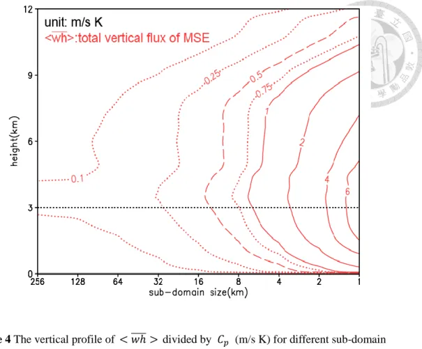
Figure 4 The vertical profile of < 𝑤ℎ̅̅̅̅ > divided by 𝐶_𝑝 (m/s K) for different sub-domain sizes (km).

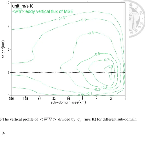
Figure 5 The vertical profile of < 𝑤̅̅̅̅̅̅ > divided by 𝐶^′ℎ^′ _𝑝 (m/s K) for different sub-domain sizes (km).

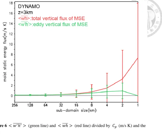
AW13 pointed out that the standard deviations of < 𝑤̅̅̅̅̅̅ > and < 𝑤ℎ^′ℎ^′ ̅̅̅̅ > in the same sub-domain size are quite large, about the scaling of variables themselves, showing that there exist significant uncertainty in the resolution dependence. The statistics of resolution dependence in DYNAMO case also show the similar results (fig. 6). Using resolution as the index of sub-grid scale convection is not an ideal method since different phases of convection are all categorized in the same groups.

Following the analyses in AW13, the convective updraft coverage ratio of each

sub-domain is used as an alternative index of sub-grid scale convection in our experiment. The convective updraft coverage ratio (denoted as σ) is defined as the number of CRM grid points with vertical velocity larger than or equal to 0.5 m/s

divided by the number of total grid points in the sub-domain (GCM-like grid). Fig. 7 is the σ dependence of < 𝑤̅̅̅̅̅̅ > and < 𝑤ℎ^′ℎ^′ ̅̅̅̅ > in the case of 4km sub-domain size at 3km height. The distribution of < 𝑤̅̅̅̅̅̅ > is likely a bimodal distribution, which ^′ℎ^′ shows that the sub-grid scale convection decline for both higher and lower σ.

Furthermore, < 𝑤̅̅̅̅̅̅ > dominates < 𝑤ℎ^′ℎ^′ ̅̅̅̅ > not only in coarser resolutions but also for lower σ in the relatively high resolutions (shown in fig. 7). For higher σ,

< 𝑤̅̅̅̅̅̅ >/< 𝑤ℎ^′ℎ^′ ̅̅̅̅ > decrease since the sub-domains themselves are more dominated

by convective updrafts, making the sub-grid scale convection more precisely resolved by grid scale processes.

Figure 6 < 𝑤̅̅̅̅̅̅ > (green line) and < 𝑤ℎ^′ℎ^′ ̅̅̅̅ > (red line) divided by 𝐶_𝑝 (m/s K) and the corresponding standard deviation for different sub-domain sizes (km).

Figure 7 < 𝑤̅̅̅̅̅̅ > (green line) and < 𝑤ℎ^′ℎ^′ ̅̅̅̅ > (red line) divided by 𝐶_𝑝 (m/s K) for different σ at 3 km height and 4km sub-domain size. Blue line is for < 𝑤̅̅̅̅̅̅ > that use the single ^′ℎ^′ top-hat assumption.

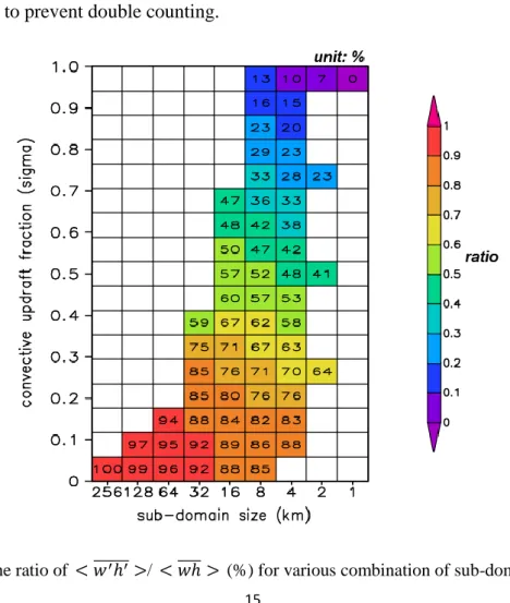
To compare the resolution dependence and σ dependence at the same chart,

< 𝑤̅̅̅̅̅̅ >/< 𝑤ℎ^′ℎ^′ ̅̅̅̅ >) of different sub-domain sizes and different σ at 3 km height are

shown in fig. 8. Similar to the results of AW13, the ratio of eddy and total vertical fluxes of MSE is more likely to be dependent on σ, rather than sub-domain sizes. If we choose < 𝑤̅̅̅̅̅̅ >/< 𝑤ℎ^′ℎ^′ ̅̅̅̅ > of sub-domain size = 4km as examples, the distribution of

ratio range from 10% for the largest σ to 88% for about σ = 0.1. If σ = 0.5 is considered, the < 𝑤̅̅̅̅̅̅ >/< 𝑤ℎ^′ℎ^′ ̅̅̅̅ > range from 41% to 57%, which is much narrower than the distribution range of sub-domain size = 4km. The ratio for other σ and heights also show the similar results, indicating that the σ dependence of < 𝑤̅̅̅̅̅̅ >/< 𝑤ℎ^′ℎ^′ ̅̅̅̅ > is

more consistent than resolution dependence. The results also show that < 𝑤̅̅̅̅̅̅ >/<^′ℎ^′ 𝑤ℎ̅̅̅̅ > of sub-domains with larger σ is smaller than those with lower σ because that if

the convective updrafts develop to sub-domain grid size, the variables of grid cell will resolve more of its sub-grid scale processes, and its degree of parameterization should be reduced to prevent double counting.

Figure 8 The ratio of < 𝑤̅̅̅̅̅̅ >/ < 𝑤ℎ^′ℎ^′ ̅̅̅̅ > (%) for various combination of sub-domain size

(horizontal axis) and σ (vertical axis) at 3km height

In the conventional cumulus parameterization, the updrafts of in-cloud and environment in the same grid cell of GCM are assumed to be homogeneous. This assumption is called single top-hat profile assumption, which means that there exists only one kind of vertical MSE flux for in-cloud and another for the environment in each GCM grid cell. In the following contents, we are going to testify this assumption in DYNAMO case by applying the analysis methods in AW13. The vertical velocity and MSE of CRM grids in each sub-domain are classified into two categories: in-cloud and environment, according to whether the vertical velocity of CRM grid is convective (w ≥ 0.5m/s) or not. For the in-cloud grids, the vertical velocities and MSE are replaced by the in-cloud average variables. These variables are used to derive the in-cloud vertical flux of MSE, and the processes are also

conducted for those environment grids to derive the environment vertical flux of MSE.

< 𝑤̅̅̅̅̅̅ > and < 𝑤ℎ^′ℎ^′ ̅̅̅̅ > that are modified by the single top-hat assumption are calculated and plotted with σ index (shown as the blue line in fig. 7). The difference

between green and blue lines is mainly attributed to the multi-structure of in-cloud grid cells for large σ. Although the single top-hat assumption used in conventional

parameterization underestimates the sub-grid scale convection strength, this simplifying assumption still do well for sub-domains with small σ, which are the main groups of all convection samples.

The results mentioned above are the statistics of DYNAMO case including convective grids (𝑤̅ + 𝑤^′≥ 0.5m/s) for all time steps, but the difference of active

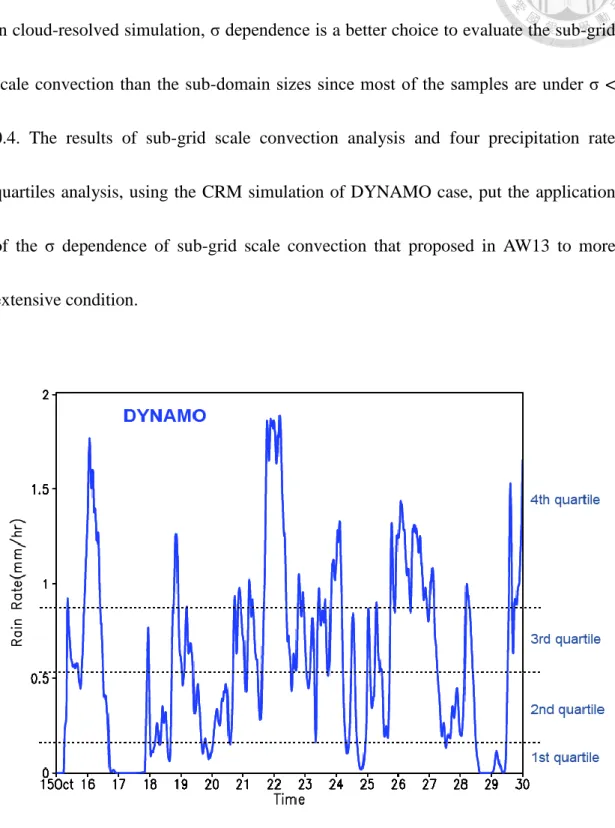
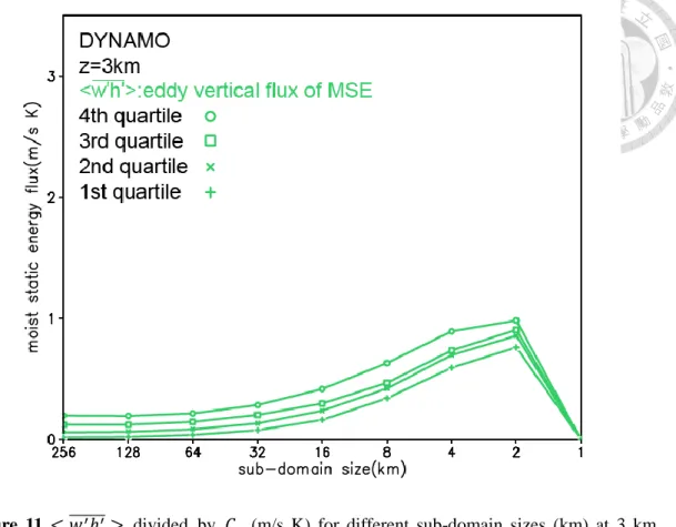
and suppress phase of convection might be covered. Xiao et al. (2015) pointed out that the resolution dependence of ZM-parameterized sub-grid scale convection is sensitive to the convection strength, implying that weaker and stronger convection might have inconsistency on resolution dependence and σ dependence. We categorize the 15-day CRM simulation data (1080 time steps) into four groups according to the domain-averaged precipitation rates (see fig. 9), and use the analysis methods of resolution and σ dependence just as we conducted to 15-day simulation before. The analysis results of these four groups of convection are shown in fig. 10 and 11. The resolution-dependent < 𝑤̅̅̅̅̅̅ > and < 𝑤ℎ^′ℎ^′ ̅̅̅̅ > rank according to their precipitation rates, indicating that the sub-domain size dependence of convection is dependent on precipitation rates. The σ dependence of four precipitation rate quartiles shown in fig.

12, 13 and 14 illustrate that < 𝑤ℎ̅̅̅̅ > (red lines), < 𝑤̅̅̅̅̅̅ > (green lines) and single ^′ℎ^′

top-hat sub-grid scale convection (blue lines) of different precipitation rates are similar to each other for σ < 0.4. Overall, for variant thermodynamic forcing applied in cloud-resolved simulation, σ dependence is a better choice to evaluate the sub-grid scale convection than the sub-domain sizes since most of the samples are under σ <

0.4. The results of sub-grid scale convection analysis and four precipitation rate quartiles analysis, using the CRM simulation of DYNAMO case, put the application of the σ dependence of sub-grid scale convection that proposed in AW13 to more extensive condition.

Figure 9 Space-averaged precipitation (mm/hr) of simulation using DYNAMO time-variant

forcing. The percentile rank of precipitation rate is showed at the right side of the chart.

Figure 10 < 𝑤ℎ̅̅̅̅ > divided by 𝐶_𝑝 (m/s K) for different sub-domain sizes (km) at 3 km height.

The data of four quartiles are shown as following marks: plus, cross, square, and circle

according to its precipitation rank.

Figure 11 < 𝑤̅̅̅̅̅̅ > divided by 𝐶^′ℎ^′ _𝑝 (m/s K) for different sub-domain sizes (km) at 3 km height. The data of four quartiles are shown as following marks: plus, cross, square, and circle

according to its precipitation rank.

Figure 12 < 𝑤ℎ̅̅̅̅ > divided by 𝐶_𝑝 (m/s K) for different σ at 3 km height. The data of four quartiles are shown as following marks: circle, square, cross and plus, according to its

precipitation rank.

Figure 13 < 𝑤̅̅̅̅̅̅ > divided by 𝐶^′ℎ^′ _𝑝 (m/s K) for different σ at 3 km height. The data of four quartiles are shown as following marks: circle, square, cross and plus, according to its

precipitation rank.

Figure 14 < 𝑤̅̅̅̅̅̅ >, that use single top-hat assumption, divided by 𝐶^′ℎ^′ _𝑝 (m/s K) for different σ at 3 km height. The data of four quartiles are shown as following marks: circle, square, cross and plus, according to its precipitation rank.

3. The derivation of unified parameterization scheme

3.1 The revision of conventional closure to unified closure

The σ dependence of sub-grid scale convection in CRM simulation implies that the cumulus parameterization with scale-awareness should parameterize the convection fluxes with bimodal distribution. AW13 derived an additional UP scheme to compensate the drawbacks of conventional parameterization scheme and make the

parameterized convection more fit to the σ dependence in CRM simulation. In conventional parameterization, with the assumption of homogeneous top-hat profile for all convective updrafts and its environment, we can express w and h of the updrafts and of the environment by 𝒘_𝒄, 𝒉_𝒄

and

between in-cloud and environment can be defined as 𝚫𝒘 ≡ 𝒘_𝒄− 𝒘̃ (1)

and

𝚫𝒉 ≡ 𝒉_𝒄− 𝒉̃, (2)

respectively. Assume that σ and σ̂ represents the convective coverage ratio of updrafts of vertical velocity and MSE respectively. The average w (𝒘̅) and MSE (𝒉̅)

of grid cell can be written as 𝒘̅ = 𝝈𝒘_𝒄+ (𝟏 − 𝝈)𝒘̃, (3)

and

𝒉̅ = 𝛔̂𝒉_𝒄 + (𝟏 − 𝛔̂)𝒉̃. (4)

In conventional schemes, the σ̂ of MSE is assumed to be small and finite. That is to say, the average MSE of sub-domain can be represented by the MSE of environment.

𝒉̅ = 𝒉̃ (5)

Including the assumption (equation (5)), the vertical eddy MSE flux in

conventional parameterization can be written as 𝒘^′𝒉^′

̅̅̅̅̅̅ = 𝒘𝒉̅̅̅̅ − 𝒘̅𝒉̅ = 𝝈𝒘_𝒄𝒉_𝒄+ (𝟏 − 𝝈)𝒘̃𝒉̃ − (𝝈𝒘_𝒄+ (𝟏 − 𝝈)𝒘̃)𝒉̃ = 𝝈𝒘_𝒄𝜟𝒉. (6)

The UP scheme closure derived by AW13 first takes back the σ̂ of MSE instead of neglecting it, and assume that the convective updrafts of vertical and MSE are

consistent, which means that 𝜎 = σ̂. The equation of 𝑤̅̅̅̅̅̅ ends up as ^′ℎ^′ 𝒘^′𝒉^′

̅̅̅̅̅̅ = 𝝈(𝟏 − 𝝈)𝜟𝒘𝜟𝒉. (7)

AW13 has mentioned that 𝜟𝒘𝜟𝒉 in CRM simulation is nearly independent of σ, thus the parameter σ(1 − σ) in equation (7) strongly restrict the < 𝑤̅̅̅̅̅̅ >^′ℎ^′ in CRM simulation to be a bimodal curve, which has minimum values for σ = 0 and σ = 1, with maximum value for about σ = 0.5. Compare the equation (7) with < 𝑤̅̅̅̅̅̅ > ^′ℎ^′ under top-hat profile assumption in figure 7, we can see that the pattern of 𝜎 dependence can be fit into this bimodal curve. For σ = 0, no convective updraft exist in the grid cell, so the sub-grid scale convection should be zero. On the other side, when σ = 1, grid cell itself is filled with “grid scale” of sub-grid scale convection, thus the convection can be directly simulated in the model. Under this condition, sub-grid scale convection should play no role on convective adjustment, or the parameterization will compose double-counting problem.

Many conventional schemes, including ZM scheme, are adjustment scheme that the vertically integrated CAPE or cloud work function is fully adjusted to the equilibrium state. The value of 𝑤̅̅̅̅̅̅ that required to fully adjust from grid scale ^′ℎ^′ forcing to equilibrium state can be written as (𝑤̅̅̅̅̅̅)^′ℎ^′ _𝐸. Use the assumptions that 𝜎 in the conventional schemes is either explicitly or implicitly assumed to be much smaller than 1, the equation of

𝝈(𝟏 − 𝝈)𝜟𝒘𝜟𝒉 = (𝒘̅̅̅̅̅̅)^′𝒉^′ _𝑬

(8)

can be rewritten as

𝝈 = (𝒘̅̅̅̅̅̅)^′𝒉^′ _𝑬/𝜟𝒘𝜟𝒉 (9)

and

(𝒘̅̅̅̅̅̅)^′𝒉^′ _𝑬 ≪ 𝜟𝒘𝜟𝒉. (10)

In this assumption, these two parameters are restricted to be in the following conditions: the grid-scale destabilization rate((𝑤̅̅̅̅̅̅)^′ℎ^′ _𝐸) should be relatively smaller or

the sub-grid scale adjustment (𝛥𝑤𝛥ℎ ) should be relatively larger. To ease this restriction, AW13 brings out a revised closure of vertical MSE flux in the UP scheme.

In the UP scheme, the equation of σ is rewritten as:

𝝈 = (𝒘̅̅̅̅̅̅)^′𝒉^′ _𝑬/(𝜟𝒘𝜟𝒉 + (𝒘̅̅̅̅̅̅)^′𝒉^′ _𝑬). (11)

This is a simpler choice to satisfy the reasonable condition: 0 ≤ 𝜎 ≤ 1. When the

flux of sub-grid scale adjustment is relatively strong (𝛥𝑤𝛥ℎ is much stronger than (𝑤̅̅̅̅̅̅)^′ℎ^′ _𝐸), this equation reduces to the conventional closure which is consist with the

assumption 𝜎 ≪ 1. On the other hand, if the stratification in the environment is stable, sub-grid scale convection should be smaller and thus 𝛥𝑤𝛥ℎ ≪ (𝑤̅̅̅̅̅̅)^′ℎ^′ _𝐸. Under this condition, 𝜎~1 , which means that the grid cell is full of weak sub-grid scale convection to adjust the larger grid scale destabilization. Combine with the original closure that without the assumption of 𝜎 (using equation (7)) and fully adjustment (using equation (11)), the closure can be written as:

𝒘^′𝒉^′

̅̅̅̅̅̅ = (𝟏 − 𝝈)^𝟐(𝒘̅̅̅̅̅̅)^′𝒉^′ _𝑬. (12)

Since 𝜎 is always larger than or equal to zero, sub-grid scale convection (𝑤̅̅̅̅̅̅) ^′ℎ^′ derived from equation (12) is a reduced value in the UP scheme. For larger 𝜎, grid cells are more dominated by sub-grid scale convection, thus double counting issue between

the sub-grid scale and grid scale convection fluxes becomes serious, and the UP scheme should play it role on reducing parameterized convection. If the resolution of refined resolution GCMs are high enough to resolve cumulus convection, the σ of convective

updrafts should all be close to 1 and the conventional parameterization in GCM can be spontaneously “turned off” and converge to the simulation of CRM.

3.2 Parameterize σ from boundary convection scheme

σ can't be directly simulated in the conventional parameterization scheme since 𝜎𝑤_𝑐 are determined together from 𝑤̅̅̅̅̅̅ without separately diagnosing, so it requires ^′ℎ^′

other parameters in the closure to derive. Remind that we actually don’t know the value of environment variables in GCMs, so 𝛥𝑤 and 𝛥ℎ (defined as the difference between updraft and environment) are first replaced by 𝛿𝑤 and 𝛿ℎ (defined as the difference between updraft, and grid cell average, which are known in GCM). Use the

definition above,

𝜹𝒘 = (𝟏 − 𝝈)𝜟𝒘, (13) 𝜹𝒉 = (𝟏 − 𝝈)𝜟𝒉, (14) and 𝜟𝒘𝜟𝒉 = 𝜹𝒘𝜹𝒉/(𝟏 − 𝝈)^𝟐

(15)

are derived out. Define

𝝀 ≡ (𝒘̅̅̅̅̅̅)^′𝒉^′ _𝑬/𝜹𝒘𝜹𝒉 (16)

the new set of equations become:

𝒘^′𝒉^′

̅̅̅̅̅̅ = (𝟏 − 𝝈)^𝟐(𝒘̅̅̅̅̅̅)^′𝒉^′ _𝑬, (17)

𝝀 = (𝒘̅̅̅̅̅̅)^′𝒉^′ _𝑬/𝜹𝒘𝜹𝒉, (18) and 𝝀(𝟏 − 𝝈)^𝟑− 𝝈 = 𝟎 (19)

To resolve 𝜆, fully adjusted MSE flux (𝑤̅̅̅̅̅̅)^′ℎ^′ _𝐸 and 𝛿ℎ is required from the conventional parameterization scheme, and 𝛿𝑤 is determined by the in-cloud vertical velocities from boundary convection scheme (De Roode et al. (2012)) minus the grid cell average vertical velocity. The equation of in-cloud vertical velocity in the

boundary convection scheme is shown below:

𝟏 𝟐

𝝏𝒘_𝒄^𝟐

𝝏𝒛 = 𝒂𝑩_𝒄− 𝒃𝜺𝒘_𝒄^𝟐

, (20)

where 𝐵_𝑐 represents buoyancy term, defined as the virtual temperature difference between in-cloud parcel and environment, and 𝜀 represents entrainment rate derived from conventional parameterization scheme. Here we use the coefficients referred from ECMWF (2010) and the coefficients 𝑎, 𝑏 equals to 1/3 and 1.95 respectively. The equation (20) is integrated from the launching level, defined as maximum MSE level, to

the theoretical convection top level, where the parcel buoyancy transfer from positive to negative, to derive the corresponding vertical kinetic energy budget.

To test the sensitivity of UP closure to the decision of in-cloud vertical velocities, we also use the vertical velocity diagnosing closure derived from Kim and Kang (2011), to compare with the one derived from ECMWF (2010). Kim and Kang (2011) use the relative humidity (RH) parameter as the alternative of entrainment rate in the convection. Under the condition of dry environment air, the entrainment of dry air will significantly slow down the up-going motion of in-cloud convection, and vice versa.

The closure of Kim and Kang (2011) are

𝟏 𝟐

𝝏𝒘_𝒄^𝟐

𝝏𝒛 = 𝒂(𝟏 − 𝑪_𝜺𝒃)𝑩_𝒄, (21) and 𝑪_𝜺 =_𝑹𝑯^𝟏 − 𝟏. (22)

where 𝒂 = 𝟏/𝟔 and 𝒃 = 𝟐.

When the buoyancy is negative, 𝑪_𝜺

is arbitrarily set to -0.25 in order to slow

is set to 0.01 when RH is

3.3 Combination with Zhang-McFarlane Scheme

ZM scheme combined with UP closure can be used to evaluate the effects of including σ dependence in the parameterization. Before going through ZM and UP scheme, the 15-day simulation of DYNAMO case is divided into different sizes of sub-domains, similar to figure 2, and then the variables are averaged in each sub-domain. The mean state variables with σ that derived from CRM larger than zero are chosen and used to trigger ZM scheme in offline test. In ZM scheme, the mass flux model calculates the updraft and downdraft mass fluxes by multiplying the cloud-base updraft mass flux 𝑀_𝑏 with a mass flux unit profile, so the decision of 𝑀_𝑏 is critical in determining the convection adjustment scaling. 𝑀_𝑏 is derived from the following

equation:

𝑴_𝒃𝑭 =^{𝒎𝒂𝒙(𝑨−𝑨}_𝛕 ^𝟎,𝟎)

, (23)

where F is the rate of CAPE removed by convection per unit 𝑀_𝑏, 𝐴 is the convective available potential energy of the current profile, 𝐴₀ is an arbitrarily defined constant that represent the equilibrium state, and τ is the constant convective adjustment time scale, usually regarded as a relaxation parameter. Parameterized MSE flux from ZM scheme will be revised in the UP scheme with the parameter 𝜎 that is derived from UP scheme closure, denoted as 𝜎_𝑈𝑃 in the following contents. The 𝜎 derived from the

directly simulation in CRM is denoted as 𝜎_𝐶𝑅𝑀 in the following contents to avoid misleading. ZM scheme that we use here is a revised version that has been introduced in Xiao et al. (2015). The original variable, 𝐴 − 𝐴₀, is revised to the difference of CAPE between the profile that the apparent forcing, advection terms, radiation, surface and PBL eddy fluxes are deducted by the time scale 600 seconds, noted as “advection

profile”, and the original profile that is assumed to be the equilibrium state, noted as

“nonadvection profile”, using the QE hypothesis proposed by Arakawa and Schubert,

1974. The dissipation rate of CAPE (F) in equation (23) and the buoyancy term and

entrainment/detrainment term for equation (20) are derived from the thermodynamic variables of “advection profile”.

In short conclusion, 𝜎_𝑈𝑃 is the function of 𝜆 (defined as (𝑤̅̅̅̅̅̅)^′ℎ^′ _𝐸/𝛿𝑤𝛿ℎ ), so the decision of (𝑤̅̅̅̅̅̅)^′ℎ^′ _𝐸 (conventional parameterized MSE flux) and 𝛿𝑤𝛿ℎ (defined as the multiplication of cloud-environment w deviation and MSE deviation) are critical to

this closure. (𝑤̅̅̅̅̅̅)^′ℎ^′ _𝐸 is revised by the new closure (equation (21)), which means that the time scale(𝜏), the anomaly of CAPE from equilibrium state (𝐴 − 𝐴₀) and the

dissipation rate of CAPE (F) can affect this value. If the value of CAPE anomaly or the dissipation rate of CAPE is negative, the corresponding vertical column will be regarded as convective stable and excluded in the following analysis. On the other hand,

the denominator 𝛿𝑤𝛿ℎ is decided by four variables,𝑤_𝑐, 𝑤̅ , ℎ_𝑐, and ℎ̅. We have mentioned above that the difference of in-cloud and environment MSE flux (ℎ_𝑐 − ℎ̅)

can be derived from the conventional scheme, while the in-cloud vertical velocity (𝑤_𝑐) should be derived from the boundary convection scheme since it’s not explicitly

parameterized. The combination of two different schemes might cause the unreasonable condition: the in-cloud vertical velocity (𝑤_𝑐) is smaller than the grid scale vertical velocity (𝑤̅), making 𝛿𝑤 less than zero. To deal with this problem, if the

multiple of 𝛿𝑤𝛿ℎ is less than zero, then the 𝜎_𝑈𝑃 corresponding to the 𝛿𝑤𝛿ℎ will be revised to 1.0. In physics 𝛿𝑤𝛿ℎ can be regarded as the consuming rate of convective instabilities by sub-grid scale convection. If the consuming rate is numerically smaller than zero, it means that the sub-grid scale convection is relatively weak and needs as more convective clouds as possible to consume the instability. For sub-grid scale convection, the largest size will be the grid itself and thus the 𝜎_𝑈𝑃 should be 1.0. More details of parameterizing processes in ZM scheme are written in Appendix.

4. Analysis of unified parameterized convection

In this section, we use the sub-domain averaged variables in DYNAMO case to run the UP scheme with offline test, and analyze the characteristics of the

UP-parameterized convection. The parameterized convection flux is basically decided by cloud-base mass flux, so we first focus on the results of LCL (lifting condensation level), where we define as cloud-base here. The values of 𝜎_𝐶𝑅𝑀 that directly derived by calculating convective grid cells in CRM simulation are also used to compare with 𝜎_𝑈𝑃, and the points that 𝜎_𝐶𝑅𝑀 equals to zero are excluded. The time steps that have larger range of 𝜎_𝑈𝑃 distribution are more representative of the multiple convection derived from UP scheme, so we choose time step = 232, about 77 hours (≈3.2 days) after the initiation of simulation, and zoom in to x=128~256 km, y=128~256 km to look closely on the patterns of squall line (bow shape pattern of convection). In fig. 15-17, we show the results of UP scheme with the in-cloud vertical velocity derived from ECMWF

(2010), and then Kim and Kang (2011) in fig. 18. The shaded colors show that larger 𝜎_𝑈𝑃 distribute close to the convective grid points (larger 𝜎_𝐶𝑅𝑀). However, if we look

closer into the value of 𝜎_𝑈𝑃 and 𝜎_𝐶𝑅𝑀 within these convective grid points (fig. 15 and

18), the larger 𝜎_𝑈𝑃 tend to appear at the downward of vertical wind shear of the largest 𝜎_𝐶𝑅𝑀 (fig. 19, right). In ZM, deep convections are always triggered in the most

unstable vertical columns, while in CRM vertical wind shear can change the vertical structure of deep convection, such as tilting and stretching. These dynamic processes can shift the updraft away horizontally from where it launched, especially for smaller

grid sizes, leading to the heterogeneous distribution of 𝜎_𝑈𝑃 and 𝜎_𝐶𝑅𝑀. The partly inconsistency of 𝜎_𝑈𝑃 and 𝜎_𝐶𝑅𝑀 may cause the UP scheme to tune down the MSE flux even if the corresponding 𝜎_𝐶𝑅𝑀 is not large. Since CAPE and 𝛿𝑤𝛿ℎ are the representative parameters in the equation (18) that decide the λ in UP closure (see section 3.2), the pattern of 𝜎_𝑈𝑃 distribution is highly related with the scaling of CAPE and 𝛿𝑤𝛿ℎ. Higher 𝜎_𝑈𝑃 tends to distribute at where CAPE is higher with lower 𝛿𝑤𝛿ℎ (fig. 16 and 17), which means that the grid-scale instability is large enough to trigger the widespread updrafts, or the adjustment by updraft is relative slow so that much ensemble members of sub-grid scale updrafts are required for. These two parameters are from two different parameterization scheme, but the derivation of 𝛿𝑤 is still highly related to the profile that used to derive CAPE.

Figure 15 The horizontal domain of 4km sub-domain size, at LCL height, about 3.2 days.

Shaded color represents the value of 𝜎_𝑈𝑃 using the in-cloud vertical velocity derived by the

method of ECMWF (2010), while the number in black grid represents the value of 𝜎_𝐶𝑅𝑀 in

percentage.

Figure 16 The horizontal domain of 4km sub-domain size, at LCL height, about 3.2 days.

Shaded color represents the value of 𝜎_𝑈𝑃, while the black contour represents the CAPE

(𝑚²/𝑠²) of 4km sub-domain, defined by Xiao, 2015 in section 3.3.

Figure 17 The horizontal domain of 4km sub-domain size, at LCL height, about 3.2 days.

Shaded color represents the value of 𝜎_𝑈𝑃, while the black contour represents the product of δw

derived by the method of ECMWF (2010) and δh (K m/s) of 4km sub-domain.

Figure 18 Similar to figure 15, but with the vertical velocities derived from Kim and Kang

(2011)

The horizontal domain of 4km sub-domain size, at LCL height, about 3.2 days

Shaded color represents the value of sigma derived from UP using the closure of Kim and Kang

(2011), while the number in black grid represents the value of 𝜎_𝐶𝑅𝑀 in percentage.

Figure 19 The horizontal domain of 1km grid size at about 3.2 days

Left: red shaded, for grid point vertical velocity at LCL height in CRM simulation that larger

than or equal to 0.5m/s; the blue contour line, convergent area at 46m height that divergence

equals to -0.0002 /s; the purple dot line, divergent area at 46m height that divergence equals to

0.0002 /s; yellow arrows represent horizontal wind vector at 46m height (5m/s for the arrow

length scale).

Right: shaded color, grid point precipitation rate (mm/hr); black contour line, grid point vertical

velocity at LCL height that larger than 0.5m/s; black dot line, grid point vertical velocity at LCL

height that smaller than -0.5m/s; yellow arrow, wind shear vector between 46m and 3000m

height (5m/s for the arrow length scale).

There are grid points with 𝜎_𝑈𝑃 = 1.0 in the selected domain (purple red color in fig. 15-18) since the numerical rule allows the situation “𝜎_𝑈𝑃 = 1.0” to exist if the

product of 𝛿𝑤 and 𝛿ℎ is less than zero. The derivation of 𝛿ℎ is contained in the conventional parameterization scheme, so it’s much more possible for 𝛿𝑤 (derived from two parameterization schemes instead of ZM scheme itself) to be less than zero.

The overview of fig. 15-18 also indicate that 𝜎_𝑈𝑃 tend to be underestimated when compared to the corresponding 𝜎_𝐶𝑅𝑀. To specifically describe the difference of 𝜎_𝑈𝑃 and 𝜎_𝐶𝑅𝑀, the spectral distribution of two parameters for 4km sub-domain size at the height of LCL, and of all 15-day simulation, is shown in fig.20. Compared to 𝜎_𝐶𝑅𝑀, the ratio of higher 𝜎_𝑈𝑃 are significantly less than the “true” solution, and the distribution of 𝜎_𝑈𝑃 at higher layer are even more concentrated within the lowest bin range as shown in fig. 21. Due to the numerical rule that “if 𝛿𝑤𝛿ℎ is less than zero, 𝜎_𝑈𝑃 equals to 1”, the ratio of the highest 𝜎_𝑈𝑃 (including 𝜎_𝑈𝑃 = 1) is much more than the

expected distribution curve.

Figure 20 The numbers of sub-domains categorized by 16 𝜎_𝑈𝑃 (green box) and 𝜎_𝐶𝑅𝑀 (red

box) bins at LCL, ranging 0 < 𝜎 ≦ 1, are divided by the total number of samples and showed

as ratio number in the chart. Noticed that there are only 16 kinds of 𝜎_𝐶𝑅𝑀 for 𝜎_𝐶𝑅𝑀> 0 in

4km sub-domain size, just the same as the categorized bin number here. (unit: ratio)

Figure 21 Same as fig. 19 but at 3km height.

Equation (18) in section 3.2 reveals the possible sources of underestimated 𝜎_𝑈𝑃 are the parameters that used to derive λ. Since CAPE and 𝛿ℎ are simply derived from the conventional parameterization scheme, the 𝛿𝑤 that derived from two inconsistent parameterization schemes might be the main sources. From the whole domain and time averaged vertical velocities derived from the closure in Kim and Kang (2011),

ECMWF (2010) and CRM simulation where 𝜎_𝐶𝑅𝑀 > 0.0 (fig. 22), we can see that since the UP scheme often overestimates the in-cloud vertical velocities (𝑤_𝑐), which

play roles in denominator in equation (18) (see section 3.2), the 𝜎_𝑈𝑃 distribute at lower range than 𝜎_𝐶𝑅𝑀. The result of using Kim and Kang (2011) to diagnose 𝜎_𝑈𝑃

(see fig. 18) is similar to the result of using ECMWF (2010) since the performance of vertical velocities at LCL of both schemes are alike. However, different results are expected at higher layers. The values of RH in advection profile are often larger than 66% because the profile in the selected DYNAMO case is mostly wet, and advection moisture terms are also unconsciously added to the original profile. The in-cloud vertical velocities of Kim and Kang (2011) method at higher layers lack of dry air entrainment and thus are much larger than the ones from ECMWF (2010) and the simulation of CRM.

Figure 22 The vertical profile of averaged vertical velocity in DYNAMO case for two kinds of

solution in CRM simulation (yellow line). The samples for averaging are the whole domain of

4km sub-domain size grids that 𝜎_𝐶𝑅𝑀 > 0.0 in all time steps.

The comparison of sub-grid scale convection fluxes simulated in CRM (< 𝑤̅̅̅̅̅̅^′ℎ^′_𝐶𝑅𝑀 >), parameterized by ZM scheme (< 𝑤̅̅̅̅̅̅^′ℎ^′_𝑍𝑀 >) and adjusted by UP scheme (< 𝑤̅̅̅̅̅̅^′ℎ^′_𝑈𝑃 >) in 4km sub-domain size are shown in fig. 23. According to

equation (17) in section 3.3, the sub-grid scale convection fluxes derived from ZM scheme (𝑤̅̅̅̅̅̅^′ℎ^′_𝑍𝑀) are adjusted in UP scheme by multiplying the factor (1 − 𝜎_𝑈𝑃)²

and denoted as 𝑤̅̅̅̅̅̅^′ℎ^′_𝑈𝑃. The distribution of 𝜎_𝑈𝑃 that concentrate at lower range

implies that the difference of < 𝑤̅̅̅̅̅̅^′ℎ^′_𝑈𝑃 > (short dash line) and < 𝑤̅̅̅̅̅̅^′ℎ^′_𝑍𝑀 > (long dash line) is relatively small since the averaged (1 − 𝜎_𝑈𝑃)² is near 1. The large

difference between < 𝑤̅̅̅̅̅̅^′ℎ^′_𝐶𝑅𝑀 > and < 𝑤̅̅̅̅̅̅^′ℎ^′_𝑍𝑀 > is mainly due to the closure that decides the adjustment rate in ZM scheme, so the application of UP scheme can give little help on converging the scaling of sub-grid scale convection derived from CRM and ZM. The main purpose of UP scheme is to tune down the sub-grid scale convection if its’ corresponding 𝜎_𝑈𝑃 can’t be neglected as the conventional parameterization do. Fig. 24 show the σ dependence of 𝑤̅̅̅̅̅̅^′ℎ^′_𝐶𝑅𝑀 that we derived in section 2, and of the 𝑤̅̅̅̅̅̅^′ℎ^′_𝑍𝑀 and 𝑤̅̅̅̅̅̅^′ℎ^′_𝑈𝑃. Noticed that the σ used in horizontal axis

for 𝑤̅̅̅̅̅̅^′ℎ^′_𝐶𝑅𝑀 (𝜎_𝐶𝑅𝑀) and for 𝑤̅̅̅̅̅̅^′ℎ^′_𝑍𝑀 and 𝑤̅̅̅̅̅̅^′ℎ^′_𝑈𝑃 (𝜎_𝑈𝑃) are different as the σ realized in CRM and ZM are derived by respective methods. Before applying UP

scheme, 𝑤̅̅̅̅̅̅^′ℎ^′_𝑍𝑀 is more likely independent to the 𝜎_𝑈𝑃, while after the adjustment, 𝑤^′ℎ^′

̅̅̅̅̅̅_𝑈𝑃 for higher 𝜎_𝑈𝑃 is tuned down.

Figure 23 The vertical profile of < 𝑤̅̅̅̅̅̅^′ℎ^′_𝐶𝑅𝑀 > (solid line), < 𝑤̅̅̅̅̅̅^′ℎ^′_𝑍𝑀> (long dash line)

and < 𝑤̅̅̅̅̅̅^′ℎ^′_𝑈𝑃 > (short dash line), divided by 𝐶_𝑝 (m/s K), of 4km sub-domain size that

𝜎_𝐶𝑅𝑀 > 0.0 in all time steps in DYNAMO case.

Figure 24 < 𝑤̅̅̅̅̅̅^′ℎ^′_𝐶𝑅𝑀> (green line), < 𝑤̅̅̅̅̅̅^′ℎ^′_𝑍𝑀> (yellow line) and < 𝑤̅̅̅̅̅̅^′ℎ^′_𝑈𝑃> (blue

line) divided by 𝐶_𝑝 (m/s K) for different σ at LCL and 4km sub-domain size.

5. Conclusion and future work

Arakawa and Wu (2013) regarded the convective updraft fraction (σ) dependence of vertical eddy MSE flux in CRM simulation as a solution of parameterizing sub-grid scale convection in variant-resolved GCMs, and also applied σ dependence in the derivation of unified parameterization closure. Instead of using GATE, whose forcing terms are invariant with time, as the analyzed case in AW13, we use DYNAMO case

that applies time-variant forcing terms in the simulation to represent different phases of convection development cycles. The analysis of σ dependence of convection in DYNAMO is similar to the convection in GATE, so this parameter is also appropriate for unified expression of sub-grid scale convection in variant forcing cases. We also compare the σ dependence of different convection strength in the simulation of DYNAMO case. Variables of all time steps in CRM simulation are categorized into four groups according to the precipitation rates. It shows that within all groups of convection, σ dependence are less variant than resolution dependence, thus σ dependence is also an appropriate parameter for various strength of convection.

A UP closure, using the parameter σ and some variables output from the conventional parameterization, is derived in AW13. This closure uses σ to relax the full adjustment convection fluxes in conventional parameterization scheme because the σ in conventional parameterization is usually assumed to be much smaller than 1 and thus can be neglected. Theoretically, when the σ become closer to 1, the grid-scale variables should perceive significant components of sub-grid scale convection, so the sub-grid scale convection shouldn’t be as large as the condition when σ is ignorable, or it will double-count the convection fluxes both in grid-scale and sub-grid scale. Numerically, the UP closure multiplies the convection fluxes by

(1 − σ)², which means that if the convective updraft is close to grid-scale, the role of

sub-grid scale convection can almost be neglected. For the GCM with the resolution

of CRM, the function of parameterization can be smoothly “closed” when multiplying (1 − σ)² because all convection fluxes in the simulation are grid scale. In our

research, we combine a conventional cumulus convection parameterization:

Zhang-McFarlane parameterization scheme, with the UP closure in AW13, to diagnose the unified convection fluxes in the simulation of DYNAMO. The average variables of sub-domain in DYNAMO are input to ZM scheme to parameterize sub-grid convection fluxes and use σ derived from UP closure to adjust the convection fluxes. We use the ratio of ZM parameterized convection fluxes, and the multiplication of in-cloud moist static energy and the in-cloud vertical velocity derived from the boundary convection parameterization (VKE budget) to derive σ.

This convection fluxes can also be recognized as the consumption rate of environment instability by the parameterized in-cloud convection.

The result shows that the distribution of σ derived from UP closure performs better at cloud-base (here defined as LCL) than higher layers, but still have some inconsistence in both scale and position with the σ derived from CRM simulation.

This situation could be result from the triggering mechanics in conventional

parameterization, since it decides the CAPE and parameterized convection fluxes, and the coefficients and closure of in-cloud vertical velocity. The ensemble averaged sub-grid scale convection fluxes derived from UP scheme are similar to the ones from

ZM scheme since 𝜎_𝑈𝑃 are concentrate at lower values, making the adjustment parameter (1 − σ)² close to 1, and also far from the fluxes derived from CRM. The

main purpose of UP scheme is to put the awareness of σ into the parameterized convection fluxes, so the relaxation adjustment for parameterized fluxes at higher σ has shown the effects of UP scheme. The gap between fluxes in CRM and UP is mainly attributed to the closure in ZM scheme, which can relax or strengthen the adjustment rate by its closure. The possible progression in the future might be the methods to deal with tilting convection, the coefficients of in-cloud vertical velocities and the closure to decide the strength of cloud base mass fluxes.

References

Arakawa, A. 2004. The cumulus parameterization problem: Past, present, and future. Journal of

Climate, 17(13), 2493-2525.

――, J. H. Jung, and C. M. Wu, 2011. Toward unification of the multiscale modeling of the

atmosphere. Atmospheric Chemistry and Physics, 11(8), 3731-3742.

――, and W. H. Schubert, 1974. Interaction of a cumulus cloud ensemble with the large-scale

environment, Part I. Journal of the Atmospheric Sciences, 31(3), 674-701.

――, and C. M. Wu, 2013. A unified representation of deep moist convection in numerical modeling of

the atmosphere. Part I. Journal of the Atmospheric Sciences, 70(7), 1977-1992.

Collins, W. D., P. J. Rasch, B. A. Boville, J. J. Hack, J. R. McCaa, D. L. Williamson, J. T. Kiehl, B.

Briegleb, C. Bitz, S. J. Lin, and M. Zhang, 2004. Description of the NCAR community

atmosphere model (CAM 3.0). NCAR Tech. Note NCAR/TN-464+ STR, 226.

de Roode, S. R., A. P. Siebesma, H. J. Jonker, and Y. de Voogd, 2012. Parameterization of the vertical

velocity equation for shallow cumulus clouds. Monthly Weather Review, 140(8), 2424-2436.

Fan, J., Y. C. Liu, K. M. Xu, K. North, S. Collis, X. Dong, G. J. Zhang, Q. Chen, P. Kollias, and S. J.

Ghan, 2015. Improving representation of convective transport for scale‐aware parameterization: 1.

Convection and cloud properties simulated with spectral bin and bulk microphysics. Journal of

Geophysical Research: Atmospheres, 120(8), 3485-3509.

Jung, J. H., and A. Arakawa, 2004. The resolution dependence of model physics: Illustrations from

nonhydrostatic model experiments. Journal of the atmospheric sciences, 61(1), 88-102.

――, and ――, 2008. A three-dimensional anelastic model based on the vorticity equation. Monthly

Weather Review, 136(1), 276-294.

Kim, D., and I. S. Kang, 2012. A bulk mass flux convection scheme for climate model: description and

moisture sensitivity. Climate dynamics, 38(1-2), 411-429.

Kim, S. Y., and M. I. Lee, 2014, Evaluations of the Cloud-resolving Model in Representing Convective

Precipitation Process. 2014 년도 한국기상학회 가을학술대회 프로그램집, 235-236.

Liu, Y. C., J. Fan, G. J. Zhang, K. M. Xu, and S. J. Ghan, 2015. Improving representation of convective

transport for scale‐aware parameterization: 2. Analysis of cloud‐resolving model

simulations. Journal of Geophysical Research: Atmospheres, 120(8), 3510-3532.

Lappen, C. L., and D. A. Randall, 2001a. Toward a unified parameterization of the boundary layer and

moist convection. Part I: A new type of mass-flux model. Journal of the atmospheric

sciences, 58(15), 2021-2036.

――, and ――, 2001b. Toward a unified parameterization of the boundary layer and moist convection.

Part II: Lateral mass exchanges and subplume-scale fluxes. Journal of the atmospheric

sciences, 58(15), 2037-2051.

――, and ――, 2001c. Toward a unified parameterization of the boundary layer and moist convection.