尺度平均對等性檢定於基因改造產品統計評估之研究

國立臺灣大學生物資源暨農學院農藝學研究所 生物統計學組碩士論文

Division of Biometry Graduate Institute of Agronomy College of Bioresources and Agriculture

National Taiwan University Master Thesis

尺度平均對等性檢定於基因改造產品統計評估之研究

A Study on Applications of the Scaled Average Equivalence Test to Statistical Evaluation of Genetically Modified Products

朱亭甄 Ting-Chen Chu

指導教授：劉仁沛 博士 Advisor: Jen-Pei Liu, Ph.D.

中華民國 102 年 6 月

June, 2013

i

誌謝

在台大農藝所生統組碩士班的這兩年讓我受益良多，由衷感謝我的指導老師 劉仁沛教授。自大學部開始加入劉老師的研究室之後，即感受到老師的教學熱忱 和對學生的無私奉獻，進入碩士班之後，更是受到劉老師不辭辛勞的指導與孜孜 不倦的叮嚀，使我能順利完成碩士班學業並且完成碩士論文，並且給予了我不僅 在學業上，甚至在為人處事這方面上學習、成長了許多，再次誠實感謝劉仁沛老 師!也感謝兩位口試委員 林志榮 助理教授和 季瑋珠 教授，感謝您們給予我的建 議和指導，使我的碩士論文更為完善!

而在碩士班的兩年生涯中，因為有了研究室學長姐、同儕、以及學弟妹們的 關懷與照顧，使我感受到研究室就像一個大家庭一般溫馨。感謝姜杰學長總是很 願意幫助學弟妹解決課業上的問題，感謝瑱芳學姐、詩婷學姐總會貼心得提醒我 們許多事項，感謝同儕育誠、松林、智揚，因為有了你們一起打拚的好夥伴，使 我的碩士生涯不孤單，也感謝宇晴、力維、証群、家康在平時熱心的幫忙!

最後，我要感謝我的家人，感謝爸爸媽媽的支持與栽培，我才能完成台大碩 士學業，感謝兩位哥哥在平時不斷給予我鼓勵，並且在我人生的道路上指引方向!

亭甄 謹誌於 國立台灣大學農藝學研究所生物統計組 中華民國壹零貳年陸月

ii

摘要

根據歐盟委員會 (European Commission)，植物或動物經由人工進行基因轉植 之後，使其擁有新的特性或性質者，稱為基因改造生物 (genetically modified organisms, GMOs)。然而，隨著基改作物的發展，基改作物的安全性評估成為一大 重要議題。基改作物的成分、基因型、外表型皆需要接受評估與鑑定。

歐盟食品安全管理局 (European Food Safety Authority, EFSA) 提出了針對基 因改造作物安全性的統計考量評估方法。基改作物團隊 (GMO Panel) 建議同時利 用差異性檢定 (proof of difference) 以及對等性檢定 (proof of equivalence) 來進行 評估，並建立其信賴區間 (confidence interval)與對等性限度 (equivalence limit) 。 歐盟食品安全管理局 (European Food Safety Authority, EFSA) 對於安全性評 估之科學統計考量建議，基改作物與其傳統作物之平均差異值應落於商業品種之 自然變異中。因此，我們提出一項新的標準，亦即利用基改作物與其相對應之傳 統作物的平均平方差異，與商業品種變異的比例，來進行基改作物安全性之對等 性評估。

在 混和效應 的模式 (mixed-effects model) 之下，我們採用大樣本修正法 (Modified Large-Sample Method, MLS) 建立線性化指標的 95% 信賴上限，作為基 改作物與其相對應傳統作物的安全性對等性評估之檢定程序。最後利用模擬資料，

以經驗型Ⅰ錯誤率和經驗檢定力來評估此一檢定程序。並以一個例子介紹本方法 之應用。

關鍵字：歐盟食品安全管理局，大樣本修正法，基因改造作物，對等性限度，95%

信賴上限

iii

Abstract

According to the European Commission, genetically modified organisms (GMOs) are organisms, such as plants and animals, whose genetic characteristics are being modified artificially in order to give them a new property. However, with the development of genetically modified organisms, the assessment of GMOs for safety is an important issue. The components, genotype and phenotype of GM plants should be identified and evaluated.

The Panel on GMOs of the European Food Safety Authority (EFSA) issued a guideline of scientific opinion on the statistical considerations for safety evaluation of GMOs in 2010. The GMO Panel of the EFSA indicated that both the proof of difference and the proof of equivalence are required for evaluation of the safety of GMOs.

The EFSA’s scientific opinion on statistical considerations for the safety evaluation suggests that the difference in average between the GM crop and its conventional counterpart lie within the natural variability which can be estimated from the commercial varieties. Therefore, we propose a new criterion for assessment of equivalence of the safety profile between the GM crop and conventional crop which is the scaled square mean difference between the GM crop and its conventional crop with the variance of commercial crops as the scaled factor.

Under the mixed-effects model, we applied the modified large-sample (MLS) method to derive the 95% upper confidence limit of the linearized criterion as the testing procedure for evaluation of equivalence in the safety profile between the GMO and its conventional crop. A simulation was conducted to investigate the performance,

iv

in terms of size and power, for the proposed procedure. A numerical example illustrates the applications of the proposed method.

Key words: European Food Safety Authority, GMO, Equivalence, Modified Large Sample Method, 95% upper confidence limit

v

CONTENTS

口試委員會審定書 ... #

誌謝 ...i

摘要 ... ii

ABSTRACT ... iii

CONTENTS ... v

LIST OF FIGURES ... vii

LIST OF TABLES ...ix

Chapter 1 Introduction ... 1

1.1 Global Development of GM Crops... 1

1.2 Issues of GM Crops ... 3

Chapter 2 Safety Assessment of GM Crops ... 9

2.1 Design of Field Experiments ... 9

2.2 Concepts of Statistical Considerations of EFSA for GMOs ... 11

2.3 Two One-sided Tests (TOST) Procedure ... 13

2.4 The EFSA’s Approach... 15

Chapter 3 Proposed Method ... 23

3.1 The Linear Statistical Model for Mixed Effects Methods ... 23

3.2 The Criteria and Hypotheses ... 26

3.3 The Modified Large Sample (MLS) Approach ... 27

3.4 The MLS Upper Confidence Bound ... 28

Chapter 4 Numerical Examples ... 34

4.1 Design of the Example... 34

vi

4.2 The 95% Upper Confidence Bound ... 35

4.3 The EFSA’s Approach... 37

Chapter 5 Simulations ... 49

5.1 Specifications of Combinations of Parameters for Simulation Designs ... 49

5.2 Simulation Results ... 50

5.2.1 Empirical Size ... 50

5.2.2 Empirical Power ... 51

Chapter 6 Discussion and Conclusions ... 73

Reference ... 76

Appendix ... 78

vii

LIST OF FIGURES

Fig. 1.1 Global Area of Biotech Crops, 1996 to 2012 (Million Hectares) ... 6 Fig. 1.2 Global map of Biotech Crop countries and Mega-countries in 2012 ... 7 Fig. 1.3 Biotech Crop Areas as % of Global Area of Principal Crops, 2012... 8 Fig. 2.1 Seven possible outcomes for a single endpoint of difference testing and equivalence testing... 21 Fig. 5.1 Results of convergence about size under different numbers of sites and four different numbers of commercial varieties ... 62 Fig. 5.2 Results of convergence about size under different numbers of replicate per site and four different numbers of commercial varieties. ... 63 Fig. 5.3 Results of power with _g² 0.2 and different numbers of commercial varieties under different replicates.. ... 64 Fig. 5.4 Results of power with _g² 0.5and different numbers of commercial varieties under different replicates. ... 65 Fig. 5.5 Results of power with _g² 3and different numbers of commercial varieties under different replicates. ... 66 Fig. 5.6 Results of simulation for power with _g² 0.2 and different replicates per sites under four different numbers of commercial varieties, respectively. ... 67 Fig. 5.7 Results of simulation for power with _g² 0.5 and different replicates per site under four different numbers of commercial varieties, respectively. ... 68 Fig. 5.8 Results of simulation for power with _g² 3 and different replicates per site under four different numbers of commercial varieties, respectively.. .... 69

viii

Fig. 5.9 Response surface of power with _g² 0.2 and q=6 under 10000 simulation samples. ... 70 Fig. 5.10 Response surface of power with _g² 0.5 and q=6 under 10000 simulation samples. ... 71 Fig. 5.11 Response surface of power with _g² 3 and q=6 under 10000 simulation samples. ... 72

ix

LIST OF TABLES

Table. 2.1 Design of experiment of GM crops, non-GM crops, and commercial

varieties ... 22

Table. 3.1 Analysis of variance table for the nested mixed-effects model ... 33

Table. 4.1 Raw data of the numeric example ... 40

Table. 4.2 Analysis of variance table ... 48

Table. 5.1 Specification of parameters in simulation for size between EFSA method and MLS method ... 54

Table. 5.2 Specification of parameters in simulation for power between EFSA method and MLS method ... 55

Table. 5.3 Empirical size of the MLS method with 10000 simulation samples ... 56

Table. 5.4 Empirical size of the EFSA method with 10000 simulation samples ... 57

Table. 5.5 Empirical power of the MLS method with 10000 samples with _g² 0.2 . 58 Table. 5.6 Empirical power of the MLS method with 10000 samples with _g² 0.5 . 59 Table. 5.7 Empirical power of the MLS method with 10000 samples with _g² 3 ... 60 Table. 5.8 Empirical power of the EFSA method with 10000 samples with _g² 0.2 61

1

Chapter 1 Introduction

1.1 Global Development of Genetically Modified Crops

Genetically modified (GM) crops are those organisms what genetic materials are modified in the way through gene technology, rather than based on the natural proliferation or natural recombination under the definition of The Food Standards Committee (Codex) of United Nations Food and Agriculture Organization (FAO) and World Health Organization (WHO), and European Associates and Regulations (WHO, 2002) (EU Directive 2001/18/EC). With transgenic technology such as DNA recombination, GM crops were inserted with target genes in order to develop biotic or abiotic stress-tolerant traits. The purpose is to improve the agronomic traits, to reduce production costs, to increase production, to improve quality, or will increase the nutrients, enhance the effectiveness of the farmer farming households, and give the new value of the crop. Improved agronomic traits include insect-resistance, disease-resistance, cold-tolerance, salt-tolerance, herbicide-resistance, and other kinds of resistance. The mainstream GM traits are herbicides-resistant and insect-resistant traits. In recent years, GM crops are mainly of multiple traits hybrid (stacked traits).

Since GM crops were first commercialized in the U.S. in 1996, millions of

2

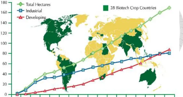
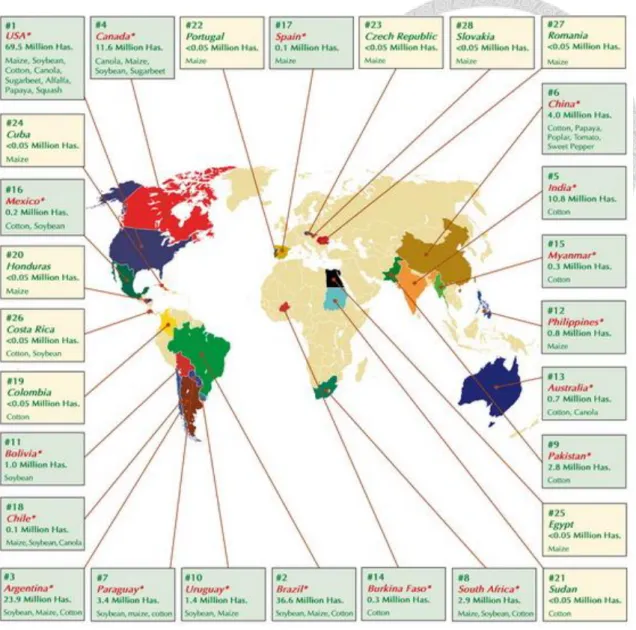
farmers worldwide have made decisions to plant and replant crops featuring the technology on an accumulated area of GM crops plantation. In 2012, the global area of GM crops continued to increase for the 17th year at a sustained growth rate of 6% or 10 million hectares (25 million acres) and to reach 170.3 million hectares or 420 million acres (Figure 1.1) (James, 2012). International Service for the Acquisition of Agri-Biotech Applications (ISAAA) data indicates that, U.S. farmers continued to plant more GM crops than any country in the world in 2011 – a total of almost 70 million hectares or 170 million acres, of which half is in the maize area, and two thirds of cotton had more than one trait, generating multiple benefits. Of the countries that had adopted biotech crops in 2012, 20 were developing countries and 8 were industrialized nations. Figure 1.2 shows the global areas of GM crops by types of countries (James, 2012). China and India lead Asian adoption, Brazil and Argentina lead Latin American adoption, South Africa leads adoption on the continent of Africa. A growth rate for GM crops in developing countries at 11 percent, or 8.7 million hectares during 2012, was significantly stronger than industrial countries at 3 percent or 1.6 million hectares.

In 2012, 81% (80.7 million hectares) of the 100 million hectares of the soybean planted globally were GM crops (Figure 1.3). GM cotton was planted to 24.3 million hectares, 81% of the 30 million hectares of global cotton, an increase from the 21.0

3

million hectares of GM cotton planted in 2010. Of the 159 million hectares of global maize planted in 2011, 35% or 55.1 million were GM maize. Finally, herbicide-tolerant GM canola was planted in 9.2 million hectares or 30% of the 31 million hectares of canola grown globally in 2012 (James, 2012). If the global areas (conventional and biotech) of these four crops are aggregated, the total area is 320 million hectares, of which 53% or 170.3 million hectares were GM crops, up from 50% in 2011.

1.2 Issues of GM Crops

In spite of benefits of GM crops mentioned above, there are serious doubts whether genetically modified crops are harmful to human, including that if transgenic genes affect human bodies, if the transgenic crops metabolites would endanger human health, and whether GM crops would impact on the environment. GM crops remain controversial because they have not been adequately tested by independent scientists.

Most of data that are the basis for government’s approval for GM crops are conducted by scientists who work either directly or indirectly for biotech companies. Moreover the data is confidential and not available for objective evaluation by independent and credible experts.

The Genetic Modified Organism Panel (GMO Panel) of the European Food

4

Safety Authority (EFSA) developed evaluation proposal for the safety of genetically modified crops in 2009. EFSA came up with the most proper field testing methods for safety assessment, as well as the use of statistical methods for the safety assessment of GM crops. GMO Panel has completed this project in December 2009 and its guideline on scientific opinion on “Statistical Consideration for the Safety Evaluation of GMOs ” has been published in 2010. It is not only the guideline for safety assessment of GM crops, but also the basic for the standardized legal formulation of GM crops by the European Union.

The EFSA scientific opinion on statistical consideration for the safety evaluation suggests the design of experiment for safety assessment, equivalence hypothesis in conjunction with the difference hypothesis, the use of natural variability of commercial varieties for establishment of equivalence limits. In addition, the EFSA’s scientific opinion proposes that the difference in average between the GM crop and its conventional counterpart should lie within the natural variability of the commercial varieties.

Following the EFSA’s scientific opinion, we propose a new criterion for assessment of equivalence of the safety profile between the GM crop and conventional crop, which is the scaled square mean difference between the GM crop and its

5

conventional crop with the variance of commercial crops as the scaled factor. Then we suggest using the 95% upper confidence bound as the testing procedure for evaluation of the equivalence between GM crop and its conventional counterpart.

Next chapter will review the statistical methods including designs recommended by the EFSA’s scientific opinion. Our proposed criterion and inference procedure are introduced in Chapter 3. Numerical examples are provided in Chapter 4 to illustrate our proposed approach and the EFSA’s method. Simulation results are reported in Chapter 5.

Chapter 6 provides the discussion and conclusions.

6

Figure 1.1 Global Area of Biotech Crops, 1996 to 2012 (Million Hectares) Source: James (2012).

7

Figure 1.2 Global map of Biotech Crop countries and Mega-countries in 2012 Source: James (2012).

8

Figure 1.3 Biotech Crop Areas as % of Global Area of Principal Crops, 2012 (Million Hectares)

Source: James (2012)

9

Chapter 2 Safety Assessment of GM Crops

2.1 Design of Field Experiments

The EFSA proposed that field trials must be set in a number of sites, and each of varieties should be randomized in plot of multiple blocks. The interaction of environment and genotype must be considered. If the interaction exists, the efficiency of statistic test holds under enough replications. As a practical consideration, commercial variables as the basis of the minimum recommended number of sites on the test set. The EFSA suggests each field experiments must be repeated in at least eight sites, where can be representative of the crop growth under environmental conditions. In addition, the environmental variability is not only variation from region to region, as well as the variability between years. The main concern is not environmental variability within each region, but that under different environmental conditions, whether the potential variability of the test material changes. The EFSA concludes if the test sites only cover

limited geographical environment, it is necessary to repeat the test more than a year.

It’s very important to choose commercial varieties while setting equivalence

limits. Varieties should represent the growth regions which in terms represent environments. The EFSA suggests that the commercial varieties should be randomized

10

in blocks besides GM crops and its conventional counterparts. In addition, the GMO Panel proposed at least six commercial varieties is necessary within a field trial to provide sufficient natural variation.

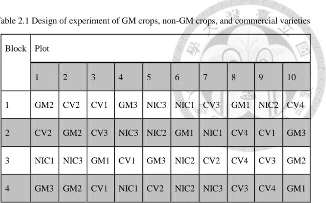
The EFSA recommended that the GM crops, conventional counterparts, and commercial varieties should be randomized within each of block in the field trial. On the other hand, the EFSA also suggested that (1) each of the appropriate conventional counterpart(s) must always together with its particular GM crop in the same block, (2) all the different GM crops and their conventional counterpart(s) and all the commercial varieties used for test equivalence with those GM crops must be fully randomized within each block. For example, in the same field trial plot, GM1, GM2, and GM3 represent three different GM crops; NIC1, NIC2 NIC3 are relatively non-GM crops;

CV1, CV2, CV3, CV4 are four commercial varieties. Based on the trial of a minimum replicate number of four, an example of experiment design is as Table 2.1.

It is worth noting that the terms of the idea of degrees of freedom in the statistical point of view, all the information in the field trials should be placed in a test assessments, which can achieve the most effectively reduce the baseline residual.

However, the GMO Panel proposed GM crops should be individually assessed due to the need to maintain transparency and verifiability. Therefore, for example, for the

11

design given in Table 2.1 to assess GM1, only plot 2,3,6,7,8,10 test data points in a the area set can be placed into the assessment consideration; To assess GM2, only plot 1,2,3,7,9,10 data points can be placed in the assessment consideration.

2.2 Concepts of Statistical Considerations of EFSA for GMOs

“Statistical Consideration for the Safety Evaluation of GMOs, EFSA, 2010”

updated statistical guidelines and possible approaches for the analysis of compositional, agronomic and phenotypic data from field trials carried out for the risk assessment of GM plants and derived foods/feeds, and provided minimum requirements that should be met in the experimental design of field trials such as the inclusion of commercial varieties, in order to ensure sufficient statistical power and reliable estimation of natural variability. It suggests the safety assessment of GM products with the use of statistical methods for comparisons between GM products and non-GM products, and between GM products and commercial products which have been listed with security history. It is recommended to quantify natural variability from data on non-GM commercial varieties treated in the same way and in the same experiments as the GM and the conventional counterpart test materials. The main concept is the comparative assessment to demonstrate whether the GM products and/or derived food/feed are

12

different from their appropriate conventional counterparts and/or equivalent to commercial varieties, apart from the inserted traits. Comparisons should consider genotype, phenotype, composition, gene location characteristics, and other unique agronomic traits.

Instead of completely accepting or completely rejecting the null hypothesis that there is difference between GM crop and its counterpart variety from test results, the EFSA provides a richer frame work within which the conclusions of both types of assessment are allowed because statistical methodology should not be focused exclusively on either differences or equivalences. Statistically significant differences may point at biological changes caused by the genetic modification, but may not be relevant from the viewpoint of food safety. On the other hand, equivalence assessments may identify differences that are potentially larger than normal natural variation, but such cases may or may not be cases where there is an indication for true biological change caused by the genetic modification. A procedure combining both approached can only aid the subsequent toxicological assessment following risk characterization of the statistical results. The GMO Panel proposed the use of confidence intervals can be described more messages between GM crops and its control counterpart varieties.

The concept of equivalence must be clarified clearly, which is defined as

13

“absence of differences ", rather than the general biological variability or differences

caused by genetically modified. In order to test equivalence in a statistically rigorous manner, it is necessary to specify for each tested variable a maximum acceptable difference, set either as the difference  between the GMO and its conventional counterpart, or as the difference ' between the GMO and the mean of commercial

reference varieties. In principle the limits on the difference can be different in the positive and the negative direction; these are termed, respectively, the ‘upper equivalence limit’, _U , and the ‘lower equivalence limit’, _L。

2.3 Two One-sided Tests (TOST) Procedure

When testing for differences (proof of difference approach) the null hypothesis and alternative hypothesis are:

0: _{G C} 0

H    (2.1)

: 0

a G C

H    ,

where  _G( _C) is the population mean of the GM (its conventional counterpart) crop.

In words, the null hypothesis is “no difference between the GMO and its conventional counterpart” against the alternative hypothesis: “difference between the GMO and its conventional counterpart”. This is a common two-tailed test for detecting on the both

14

direction of incremental and decreasing value. However, the difference of endpoint only to fall in ascending or descending one end, one-tailed test should be used at this time.

For each test with significance level 1 (e.g. 95 %), there is a limited Type I error probability ( , the size of the test) that a significant result is obtained (i.e. a difference is found) whereas no difference exists in reality. However, these tests do not restrict the Type II error probability () of finding no significance whereas in reality there is a

difference. So the absence of significant results is not a proof for equivalence of the GMO and the conventional counterpart, or ‘‘absence of evidence is not evidence of absence’’ (Altman and Bland, 1995, 2004).

Schuirmann (1987) proposed a new approach to this problem. The objectives of assessment of equivalence may be formulated into the following statistical hypotheses:

0: _{G C L}

H    or _G_C _U (2.2)

: _{L G C U}

Ha     ,

where is the lower bound for equivalence; is the upper bound for equivalence.

It is the interval hypothesis, which can be decomposed into two sets of one-sided hypotheses:

01: _{G C L}

H   

1:

a G C L

H   

15

and (2.3)

02: _{G C U}

H   

2:

a G C U

H   

The two one-sided tests procedure rejects the interval hypothesis H , and ₀ concludes equivalence between _G and _C, if and only if both H and ₀₁ H are ₀₂

rejected at a chosen nominal level of significance  . Equivalently, FDA (2001) and EMEA (2001) propose that the (1 2 )%  confidence interval for _G_C could be constructed for the bioequivalence test.

2.4 The EFSA’s Approach

The approach which the EFSA recommended for establishment of equivalence limits is reviewed below (EFSA, 2010). In addition to the GMO and its conventional counterpart, the trials performed include several commercial crop varieties, which must represent non-GM varieties with a proven history of safe use, and these should be fully randomized as integral parts of the experiment. When commercial varieties are included in the same experiment where the GMO is tested against the conventional counterpart(s) then data on commercial varieties are obtained in identical conditions to that of the GM and its conventional counterpart. It is sensible to derive equivalence limits by

16

considering how the commercial varieties compare to the GMO. Establishment of equivalence between the GMO and its conventional counterpart has often been interpreted as relevant for subsequent toxicological risk assessments. It is recommended to apply a linear mixed-effects statistical model, fitted to (possibly transformed) data, in order to derive an estimate of variation between commercial genotypes. One model should be used for calculation of the confidence limits for both tests (difference and equivalence); a slightly different model should be used to estimate the equivalence limits to be used in the equivalence test.

Denote by I an indicator variable (uncentered in the mixed model) such that I=1 for a field plot having any of the commercial varieties, and I=0 otherwise. Then the random factors for model 1 should include, but not necessarily be restricted to, those representing the variation: (i) between the test materials (a set that includes the GM crop, its conventional counterpart, each of the commercial varieties and any additional comparators); (ii) in the interaction between the test materials and I; (iii) between sites;

and (iv) between blocks within sites. Model 2 should be identical to model 1 except that the random factor representing the interaction between the test materials and I is omitted.

For each endpoint, calculation of the confidence limits, estimation of equivalence

17

limits and associated statistical tests should be performed as described below. Sample means are denoted by Y , with subscripts G, C and R for the GM crop, its conventional counterpart and the set of commercial (reference) varieties, respectively. The variability encompassed in the standard error of the difference between the means of any two test materials, X and Y, calculated using model i (i = 1,2), is denoted sed(XY;i). The 100a%

point of Student's t distribution is denoted as t(df;i;a), where I denotes the model used and df is the appropriate number of degrees of freedom which is recommended to be calculated by the Kenward-Roger method (Kenward and Roger, 1997). The least significant difference between the means of any two test materials, X and Y, using model i, should be calculated as the product of t(df;i;a) and sed(XY;i), and is denoted lsd(XY;i;a). For the difference test, the two-sided 90% confidence limits should be calculated about Y_G, as Y_Glsd GC( ;1;95); the null hypothesis of equality between

YG and Y_C should be rejected and the test deemed statistically significant if Y_C falls outside these limits. For the equivalence test, the two-sided 95% equivalence limits should be estimated as Y_Rlsd GR( ; 2;97.5) and two-sided 90% confidence limits should be calculated about Y_G as Y_Glsd GR( ;1;95) ; the null hypothesis of non-equivalence should be rejected and the test deemed statistically significant if and only if the confidence limits lie entirely inside the equivalence limits.

18

After the appropriate transformation, simultaneous endpoints display is facilitated by shifting all relevant values for each particular endpoint to a scale that has Y_C, the mean of the conventional counterpart for that endpoint, as its baseline zero value.

Therefore, on this new scale, the values of the means of the GM crop, its conventional counterpart and the set of commercial varieties become, respectively: Y_GY_C, 0,

R C

Y Y . And the confidence limits for the difference test on this new scale become:

( ;1;95)

G C

Y Y lsd GC , the equivalence limits Y_RY_C lsd GR( ; 2;97.5) , and the confidence limits for the equivalence test Y_GY_Clsd GR( ;1;95).

To facilitate visual interpretation, instead of using the two sets of confidence limits in the graphs, it is recommended for convenience that only one be displayed, that for the difference test. Without some adjustment, the confidence limits for the difference test would not give a valid visual representation for the equivalence test on the graph.

This problem is overcome by making an adjustment to the displayed equivalence limits.

After this adjustment the displayed confidence limits for the difference test may be used as a basis also for the visual representation of the equivalence test. In this way, one confidence limit may serve visually for assessing the outcome of both tests simultaneously. The adjustment of the equivalence limits consists of two steps: (1) scaling the basic equivalence limits, so that the confidence limits required for the

19

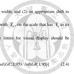
difference and equivalence tests have the same width; and (2) an appropriate shift to facilitate display of the adjusted limits, together with Y_G, on the scale that has Y_Cas its baseline zero value. The adjusted equivalence limits for visual display should be calculated by the formula:

(Y_GY_C) {[ Y_RY_G)lsd GR( ; 2;97.5)]lsd GC( ;1;95) /lsd GR( ;1;95)} (2.4)

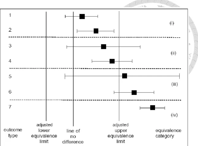
Figure 2.1 lists the possible outcomes if both approaches are considered simultaneously (EFSA, 2010). Stringent use of the concept of equivalence would require the necessity of proving equivalence for all endpoints simultaneously (global equivalence). Figure 2.1 Simplified version of a graph for comparative assessment showing the 7 outcome types possible for a single endpoint. After adjustment of the equivalence limits, a single confidence limit (for the difference) serves visually for assessing the outcome of both tests (difference and equivalence). Here, only the upper adjusted equivalence limit is considered. Shown are: the mean of the GM crop on an appropriate scale (square), the confidence limits (whiskers) for the difference between the GM crop and its conventional counterpart (bar shows confidence interval), a vertical line indicating zero difference (for proof of difference), and vertical lines indicating adjusted equivalence limits (for proof of equivalence). For outcome types 1, 3 and 5 the

20

null hypothesis of no difference cannot be rejected: for outcomes 2, 4, 6 and 7 the GM crop is different from its conventional counterpart. Regarding interpretation of equivalence, four categories are identified: in category (i) the null hypothesis of non-equivalence is rejected in favor of equivalence; in categories (ii), (iii) and (iv) non-equivalence cannot be rejected. More detailed explanations about (ii), (iii) and (iv) can be found in EFSA (2010).

21

Figure 2.1 Seven possible outcomes for a single endpoint of difference testing and equivalence testing.

Source: EFSA (2010)

22

Table 2.1 Design of experiment of GM crops, non-GM crops, and commercial varieties Block Plot

1 2 3 4 5 6 7 8 9 10

1 GM2 CV2 CV1 GM3 NIC3 NIC1 CV3 GM1 NIC2 CV4

2 CV2 GM2 CV3 NIC3 NIC2 GM1 NIC1 CV4 CV1 GM3

3 NIC1 NIC3 GM1 CV1 GM3 NIC2 CV2 CV4 CV3 GM2

4 GM3 GM2 CV1 NIC1 CV2 NIC2 NIC3 CV3 CV4 GM1

Source: EFSA (2010)

23

Chapter 3 Proposed Methods

The EFSA scientific opinion on statistical consideration for evaluation of equivalence in safety profile between the GM crop and its conventional counterpart suggests that the mean difference between the GM crop and its conventional counterpart lie within the natural variability of the commercial varieties.

In this chapter, based on the concept of scaled average bioequivalence (Patterson and Jones, 2012), we propose a new criterion for assessment of equivalence between the GM crop and its conventional counterpart which is the scaled square mean difference between the GM crop and its conventional crop with the variance of commercial crops as the scale factor. Then the modified large sample (MLS) method (Lee, et al., 2004) is applied to obtain the ((1)% upper confidence limit for the linearized criterion which is used as the testing statistics for the hypothesis based on the proposed criterion.

3.1 The Linear Statistical Model for Mixed-Effects Models

We use the mixed-effects model proposed by EFSA for the data. Let Y_ijkl denote the response, possibly logarithmically transformed, of replicate j within site i for treatment k and genotype l ; j1, 2...,p, i1, 2,...,n, k 1, 2,3(1:conventional

24

counterpart; 2: GM crops; 3: commercial variety), l1, 2,...,q. The following nested mixed-effects model is suggested by the EFSA (2010).

( )

ijkl i i j k l ijkl

y    e r   t g 

where

: mean of observations

 , e: environment (site), e_i ~ N(0,_e²)

2

: replication per site, r( )_{i j} ~ (0, _r)

r N  ,

3

1

: treatment, _k 0

k

t t





k=1: conventional variety, k=2: GMO, k=3: commercial varieties : genotype of commercial varieties, g ~_l (0, _g2)

g N  , : residuals, _ijkl ~N(0,_²)

Define

 y_; ˆe_i y_iy_; rˆ_{( )i j}  y_ijy_i; t^ˆ_k y_{ k} y_; gˆ_l  y_3ly_{ 3} ; ˆ_ijkl y_ijkly_{i kl}

Where

3 q

k l ijkl ij

y y



 

3

p q

j k l ijkl i

y y^ 

  

, mean of the observations in ith site,

3

n p

i j ijkl l

y y^ 

 

, mean of the observations of commercial variety with l th genotype,

25

n p q

i j l ijkl k

y y^{ } 

  

mean of the observations of k th treatment, and

3

n p q

i j k l yijkl

y^ 

   

, overall mean, and

s=q+(k-1).

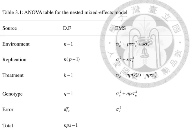
The sums of squares, degree of freedom, and the expected value of its corresponding mean square for environment, replication, treatment, genotype, and errors are given

respectively as follows:

( )2

n i i

SSe ps



( )2

n p

ij i

i j

SSrs



3

( _k )2 k

SStnp



2

3 3

3 ( )

q l l

SSgnp



3

( )2

p q

n

ijkl i kl

k i j l

SSE



E MSE _

The corresponding ANOVA table for the nested mixed-effects model is provided in Table 3.1.

26

3.2 The Criteria and Hypotheses

Since the EFSA scientific opinion for safety assessment for GM crop requires the average difference between the GM crop and its conventional counterpart should not exceed the natural variation of commercial variation, based on the concept of scaled average bioequivalence (Patterson and Jones, 2012), we propose the following scaled

average criterion:

2

2

( _{G C})

g

 

 

  (3.1)

Where _G (_C) is the average of the GM (conventional) crop and ²_g is the variance of the commercial varieties. It follows that the hypothesis for evaluation of equivalence between the GM crop and its conventional counterpart is given as

0: 0

H   vs. H_a:  ₀, (3.2) where ₀ is the equivalence limit which that the maximally allowable natural

variability of the commercial varieties to claim equivalence between the GM crop and its conventional counterpart.

Following the linearized criterion for individual bioequivalence (IBE) proposal by

Hyslop, et al. (2000), we also can formulate  into the following linearized criterion

2 2

( _{G C}) 0 _g

     (3.3)

27

As a result, hypothesis in Equation (3.2) can be re-formulated as

0: 0

H  vs. H_a:0 (3.4) Hyslop et al. (2000) also suggest using the (1)% upper confidence bound derived by the MLS method as a test statistic for hypothesis (3.4)

3.3 The Modified Large-Sample (MLS) Approach

The MLS method from Lee et al. (2004) and Hyslop, et al. (2000) is briefly reviewed as follows:

Consider the problem of setting a (1)100% confidence bound for

2 2

1 1 p p

c c

     , where ₁²,,²_p are unknown variance components and

1, , _p

c c are known nonzero constants. Let ˆ_i² be an unbiased estimator of _i² such that L(ˆ_i²)L(_i²n X_i^1 _i), where ( ) ²

i ni

L X  , i 1, ,p. ˆ_i² is a quadratic forms of

an observed normal random vector. The extension builds on the fact that the quadratic form c₁ˆ₁²c_pˆ²_p may have a chi-squared representation in the sense that

2 2 1 1

1ˆ1 ˆ 1 1 1

( _{p p}) ( _{p p p})

L c c  L v X^  v X^

where X₁,,X_P are independent chi-squared random variables with v degrees of _i freedom and _i's are unknown parameters. In addition, the number of independent chi-squared random variables is the same as the number of ˆ_i². The results can be

28

extended to the situation where c₁ˆ₁²c_pˆ²_p can be represented in distribution by a linear combination of q( p) independent chi-squared random variables. Applying the independent linear combination_{1 1}n X^1 ₁_pn X^_p¹ _p , the MLS upper and lower confidence bounds could be obtained as below

2 2 2 1 2 2 2

1 1 1

1

ˆ ˆ

ˆ _p ˆ_p ( 1) _p( ^p 1)

p

v v

c c

u u

         

, and

2 2 2 1 2 2 2

1 1 1

1

ˆ ˆ

ˆ _p ˆ_p ( 1) _p( ^p 1)

p

v v

c c

l l

         

, where ˆ_i is a consistent estimator of _i, i 1, ,p,

2 , 2 1 ,

, if 0 , if 0

i

i

v i

i

v i

u ^



 

_ 

 

 

 

, and

2 , 2 1 ,

, if 0 , if 0

i

i

v i

i

v i

l ^



 

_ 

 

 

 

2 ,v_i

 is the (1)% upper percentile of chi-square random variable with v degrees _i of freedom.

3.4 The MLS Upper Confidence Bound

Let Y_G and Y_C denote the average of the GM crop and its conventional counterpart, respectively.

29

Since

( _ijkl) ( _i ( )_{i j k l ijkl}) _k E Y E  e r   t g    t

( )

( )

2 2 2 2

( ) ( )

= ( ) ( ) ( ) ( ) ( )

=

ijkl i i j k l ijkl

i i j k l ijkl

e r g

Var Y Var e r t g

Var e Var r Var t Var g Var



 



   

     

   

  

Define

2

1 ^{n p}

G ij l

i j

Y y

 np



i j

Y y

 np



It follows that

2

2 2 2

( ) 2

2 2 2

( ) ( ) ( )

1 ( )

1 ( ),

n p

i j ij l

G ij l

i i j ij l

e r

y np

Var Y Var Var y

np n p

Var e r np

np ^



  

 

  

  

 

1

2 2 1

( ) 1

2 2 2

( ) ( ) ( )

1 ( )

1 ( ),

n p

i j ij l

C ij l

i i j ij l

e r

y np

Var Y Var Var y

np n p

Var e r np

np ^



  

 

  

  

 

2 2 2

( _{G C}) ( _G) ( _C) 2 ( _{e r} )

Var Y Y Var Y Var Y

np   ^

      , and

2

2 2 2

[ ( )] [ 2 ( ( 1) ( 1) )]

2 ( ).

G C

e r

E Var Y Y E MSe p MSr p s MSE

np s

np   ^

     

  

30

Then Y_GY_C follows a normal distribution with mean t_G t_C and variance 2 ² npt , where t_Gt_Cis denoted as _G_C and _t² _e²_r²_²

From Table 3.1, the ANOVA unbiased estimator of _e², _r², and _² are given as ˆ_e2 MSe MSr

  ps^ , ˆ_r² MSr MSE

  ^s , and ˆ_² MSE.

It follows that an unbiased estimator of _t² is given as

2 2 2 2

ˆ ˆ ˆ ˆ

1 [ ( 1) ( 1) ].

t e r

MSe MSr MSr MSE ps s MSE

MSe p MSr p s MSE ps

   

 

  

    

(3.5)

In addition, MSe , MSr , and MSE are mutually independent with the following distributions

2 2 2

2 ( 1)

~ 1

e r

n

ps s

MSe n

 ^  ^   _

 ,

2 2

2 ( ( 1))

~ ( 1)

r n p

MSr s

p n

 ^   _

 , and

2 2 ( )

~ _df .

MSE df ^





 

On the other hand, an ANOVA unbiased estimator of _g² is given as ˆ_g2 MSg MSE

  np^ (3.6) where

31

2 2

2 ( 1)

~ .

1

g q

MSg np

q

 

 _





The deviation of 100(1)% MLS upper confidence bound for (_G_C)²_g²

by the MLS method is given as follows:

Let A(Y_GY_C)², and B is the unbiased estimator of ₀ ² ( ⁰)

[ ]

g MSg MSE

np

  ^

  

Denote the A as the _U 100(1)% upper bound of Y_GY_C, then

2 2

1 2,2( 1)

[ ( )] .

U G C np G C

A  Y Y t_{ } Var Y Y

Define C as

2 2

2 2 2

1 2,2( 1) 2

[ ]

{[ 2 ( ( 1) ( 1) )] ( ) } .

U

G C np G C

C A A

Y Y t MSe p MSr p s MSE Y Y

 np s

 

 

        

Furthermore

2 0 0

0

2 2

1 ( 1) 2

( ˆ ) [( ) ( ) ]

[ ],

g

q df

L L MSg MSE

np np

L 

 

 

  _  

   

 

where

2 2

1 ( 0)[ _g]

np



    , and ₂ ^{0 2}. np ^

   

It follows that

2 2

1 2 2 2

1 , 1 ,

ˆ[ 1 1] ˆ[ 1]

q df

q df D





 

 

_{ } 

     ,

32

where ˆ₁ ( ⁰)MSg np

  ^ and ˆ₂ ⁰ MSE. np

 

Consequently, the 100(1)% MLS upper confidence for  is given as

ˆ A B C D.

     (3.7)

Then the null hypothesis of (3.4) is rejected at the  significance level and the safety profile of the GM crop can be claimed to be equivalent to that of its conventional counterpart if the 100(1)% MLS upper confidence bound ˆ   A B CD is smaller than 0.

33

Table 3.1: ANOVA table for the nested mixed-effects model

Source D.F EMS

Environment n1 _²pse²sr²

Replication n p( 1) _²s_r²

Treatment k1 _²npQ t( )np_g²

Genotype ^q1 _² np_g²

Error df_ _²

Total ^nps1

34

Chapter 4 Numeric Examples

In this chapter, we will demonstrate the procedure of MLS method from Chapter 3 with examples to construct the 100(1)% confidence upper bound for the linearized criterion. Assessment of safety for GM crops should be evaluated for all phenotypes, chemical components, or agricultural traits. However, we would only focus on one agricultural trait or one chemical component in order to demonstrate the MLS method and to compare the results from the approaches recommended by the EFSA scientific opinion on statistical considerations in 2010.

4.1 Design of the Example

This example considers an field trial which is repeated at eight sites. For each site, there are one GM crop, one conventional crop and six commercial varieties. the number of replicates is 4 for each site. We consider the log-transformed responses. The equivalence limit ₀ is set at 0.2 while the variance of the genotype from commercial varieties _g² is 2. In addition, the specifications of the parameter for the nested mixed-effects model in Section 3.1 are given below:

0

35

~ (0,3) , 1,...,8

e Ni i ,

~ (0,1) , 1,..., 4

r Nj j ,

0.05 , 1 (conventional counterpart) 0.05 , 2 (GM crops)

0.1 , (commercial varieties),

k

k

t k

others

 

 



~ (0, 2) , 1,..., 6

g Nl l , and

~ (0, 0.6).

ijkl N



Hence, _G_C is 0.05 0.05 0. A total of 256 responses were generated according to the rested mixed-effects model with the specifications of the distribution assumptions and parameters as described above. The raw logarithmic responses are provided in Table 4.1.

4.2 The 95% Upper Confidence Bound

The estimates of _G and _C are given as 0.4278

YC  , Y_G 0.5027

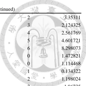
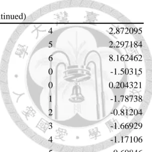
The ANOVA table is given in Table 4.2. From Table 4.2, the mean squares for environment (site), replicate, variety, genotype, and error are given respectively as

55.7653

MSe , MSr7.9580, MSt6.4432, MSg131.7064, MSE0.5843