中國對外直接投資趨勢和特徵分析

(1)

行政院國家科學委員會專題研究計畫成果報告

中國對外直接投資趨勢和特徵分析研究成果報告(精簡版)

計畫類別：個別型

計畫編號： NSC 100-2410-H-011-013-

執行期間： 100 年 08 月 01 日至 101 年 07 月 31 日執行單位：國立臺灣科技大學企業管理系

計畫主持人：張順教

計畫參與人員：碩士班研究生-兼任助理人員：梁庭郡碩士班研究生-兼任助理人員：黃奕騰碩士班研究生-兼任助理人員：江坤珉博士班研究生-兼任助理人員：林培軒

公開資訊：本計畫可公開查詢

中華民國 101 年 09 月 17 日

(2)

中文摘要：本研究主要探討自 2003 年至 2009 年間影響中國對外直接貿易(FDI)的因素。實證結果發現中國對全球的 FDI 主要受到地主國的 GDP、周圍市場潛力、空間效應、燃料出口以及擁有共同語言等因素所影響。並且發現中國 FDI 決策存在重要的第三國效應(third-country effect)。整體而言，中國對全球的 FDI 類型為複合垂直式的投資模式，中國對已開發國家的 FDI 類型亦為複合垂直式，但對開發中國家的 FDI 則是著重於周圍的市場潛力或鄰近區域龐大的第三國市場。依區域分類，中國對亞太區、非洲及歐洲國家的 FDI 類型屬複合垂直式的投資行為，而對美洲國家的 FDI 類型屬水平式的投資行為。再者，對於如石油、鋼鐵和煤礦等資源的對外投資模式，中國較傾向到開發中或非洲國家進行投資。

中文關鍵詞：對外直接投資、引力模型、空間計量、第三國效應、市場潛力

英文摘要： The study mainly investigates the features and determinants of China’s outward foreign direct investment (OFDI) into 138 countries and Chinese firms’ investment strategies from 2003 to 2009 using an augmented gravity model with spatial linkages. The respective evoluations of China’s OFDI indicate that no-financial OFDI plays an important role while

Chinese firms prefer to invest in high-tech

industries in developed countries but also approach to natural resources extraction around the world. The empirical findings show that the host economic size has a significantly positive effect in terms of

promoting Chinese ODFI but distance does not. Chinese Firms favor a complex-vertical platform while they prefer a market potential surrounding the host developing countries and an export-platform FDI for the petroleum exporting countries from spatial effects and third-country effects. The fuel

extraction movie plays a key role to China’s OFDI in line with the realities of Chinese FDI strategies in the last ten years. Finally, the appreciation policy of the currency of China to US dollar is disadvantage to China’s OFDI.

英文關鍵詞： Outward foreign direct investment, Gravity model, Spatial effects, Third-country effects

(3)

The De t e r mi nant s and Mot i vat i ons of Chi na’ s Out war d Forign Direct Investment: A Spatial Gravity Model Approach

1. Introduction

China’s forign direct investment¹

(

FDI, hereafter) flow was over US$105.74 billion in 2010 from $56.53 billion in 2009, increased 187%. (China Ministry of Commerce, 2011). The top-ranked FDI flows in 2010 were those involving the U.S., China and Hong Kong (UNCTDA, 2011). Based on estimates of the Woodrow Wilson International Center for Scholars (2011), China’stotal FDI stock aboard will reach $2 trillion by 2020 while China’s outward FDI (OFDI) into the U.S. is more than doubling annually, with nearly $5 billion in 2010 alone.

Typically, there are six characteristics of China’s OFDI. First, there are nearly Chinese 12,000 companies have directly invested 13,000 firms in 177 countries and accumulated US$245.75 billion OFDI by 2009 (UNCTDA, 2010). Rosen and Hanemann (2011) clearly concluded that Chinese OFDI policies not just focus on high-tech manufacturineg but also approach to highly intensive knowledge industries in developed countries. Secondly, China’s OFDI flows have been raising sharply since2004 whereastheaverage amountofChina’sOFDI flows were only $2.6 billion over the period from 1990 to 2003(Figure 1). Third, the non-financial China’s OFDI plays a key role. For example, the ratio of non-financial OFDI flows (stock) to total amount of OFDI flows (stock) in 2009 was 84.5% (81.3%). Fourth, as shown in Table

1 FDI is the category of international investment that reflects the objective of a resident entity in one economy (“direct investor” or parent enterprise) obtaining a ‘lasting interest’ and control in an enterpriseresidentin anothereconomy (“directinvestmententerprise”).Thetwo criteriaincorporated in thenotion of“lasting interest”are:theexistenceofalong-term relationship between the direct investor and the enterprise and, the significant degree of influence that gives the direct investor an effective voice in the management of the enterprise. The IMF threshold is 10% ownership of the ordinary shares or voting power or the equivalent for unincorporated enterprises (International Monetary Fund, IMF）.

(4)

1, the top four industries in terms of China’s OFDI stock in 2009 were Business &

Service, Finance, Mining and Wholesale & Retail Trade. The total share of top four industries was nearly 80%.

Fifth, by the view of regional point, Figure 2 exhibits that the Asian countries was the most important region to Chinese OFDI Flows while the North American and European regions had a year-to-year 3.2 and 2.8 times growth, resprectively, in 2009 (China Ministry of Commerce, 2010). The trends of China’sOFDIstockfirgured that Hong Kong , Cayman Islands and British Virgin Islands were top three regions from 2007 to 2009 (Table 2). Paritcularly, Australia, South Aferica, Macau and Kazakhstan have become top ten largest regions after 2007.

Six, government-owned companiesplay an importantrolein China’sOFDIin three decades. Following government policies, these state-owned enterprises mainly focus on the Leasing and business service(Hong Kong; EU) , Mining(Australia, Russia;

Canada; Barzil; India), Finance(Hong Kong; US), Manufactury (US), Wholesale and retailing (US; Association of Southeast Asian Nations, ASEAN) , Agriculture, forestry, husbandry and fishery (Russia) and Power and other utilities (ASEAN) (StatisticalBulletin ofChina’sOutward,2009)(Table 2).

(5)

Figure 1 China’s OFDI flows from1990 to 2009 (US$ billion)

Sources：ChinaMinsitry ofCommerce,StatisticalBulletin ofChina’sOutward(2010)

Table 1 Distribution of 2009 Chinese OFDI Stock by industry

Industry Stock (billions of US$) Share (%)

Leasing and business service 72.95 29.7

Finance 45.99 18.7

Mining 40.58 16.5

Wholesale and retailing 35.7 14.5

Transport, warehousing and postal service 16.63 6.8

Manufactury 13.59 5.5

Real estate 5.34 2.2

Construction 3.41 1.4

Science research, service and geo-survey 2.87 1.2

Power and other utilities 2.26 0.9

IT 1.97 0.8

Agriculture, forestry, husbandry and fishery 2.03 0.8 Water, enviroment and public facility

management 1.07 0.4

Residential service and other services 0.96 0.4

Residential and catering tade 0.24 0.1

others 0.16 0.1

Total 245.75 100

Figure 2 Distribution of 2009 Chinese OFDI Flows by regions

(6)

Table 2 China’s OFDI stock into major economies

Major economies Stock(billions of US$) Share (%) The share of OFDI Industries

Hong Kong 164.50 66.9

Leasing and business service (28.2%)、Finance (24.2%)、

Leasing and business service (18.6%)、Mining (13.3%)

ASEAN 9.57 3.9

Power and other utilities (19.4%)、Wholesale and retailing (17.1%)、

Manufactury (15.5%)、

Leasing and business service (10.9%)

Latin America 30.60 12.5 Cayman Islands、British Virgin Islands

U.S. 3.34 1.4

Wholesale and retailing (28.5%)、

Manufactury( 28.2%)、

Finance (14.6%)

E.U. 6.28 2.6

Leasing and business service (42.5%)、Finance 16.9%、

Mining (15.9%)、Wholesale and retailing (7.6%)

Russia 2.22 0.9

Real estate (32.1%)、

Agriculture, forestry, husbandry and fishery (24.6%)、Manufactury (12.2%)、Mining (10.1%)

Australia 5.86 2.4 Mining (85.9%)、Wholesale

and retailing (3.3%)

Tatal 222.37 90.6

Sources：ChinaMinsitry ofCommerce,StatisticalBulletin ofChina’sOutward (2009)

2. Literature background

In the context of the gravity approaches to international trade (Tinbergen, 1962;

Anderson, 1979; Bergstrand, 1985, 1989; Helpman and Krugman, 1985; Deardroff,

(7)

1998; François, 2001; Eaton and Kortum, 2002; Harrigan, 2002 and Park, 2002 among others) and FDI (Stone and Jeon, 2000 and Bénassy-Qúeŕeet al., 2001 ) , bilateral trade and investment flows depend both theoretically and empirically not only on economic mass (or country size), population, geographical distance, surrounding market potential (SMP) effect, spatial effect (third-country effect), relative exchange rate, natural resources and technical capability, but also on a common language, a common land border (adjacency) and regional trade agreements (RTAs). The recent empirical literature (Grünfeld and Moxnes, 2003; Serlenga and Shin, 2004; Naudé and Saayman, 2005; Cheng and Wall, 2005; Brun et al., 2005;

Lennon, 2006; Kimura and Lee, 2006; Antonucci and Manzocchi, 2006; Batra, 2006;

Melitz, 2007; Coe et al, 2007; Lejour and de Paiva Verheijden, 2007; Blonigen et al., 2007; Cheng and Ma, 2007; Walsh, 2008; Khadaroo and Seetanah, 2008; Garretsen and Peeters, 2009; Head et al., 2009; Jan and Jarko, 2009 and Chang and Lai, 2011 among others) has further studied the determinants of bilateral trade and FDI within an augemented gravity framework.

For instance, Blonigen et al. (2007) recognize economic size (proxied by GDP or per capita GDP) and population as being essential components of the US OFDI while Cheng and Ma(2007)havethesamefindingsin theChina’sOFDI. Grünfeld and Moxnes (2003) find that economic mass increases with bilateral trade but is inversely related to their bilateral distance (Bergstrand, 1985; Grossman, 1998; Hummels, 1999;

Cheng and Ma, 2007; Fidrmuc, 2009) and trade barriers. But the distance has a positive impact to vertival DFI and has a negative effect to horizontal FDI although an increasing distance could promote trading, investment and management costs in theory. Kimura and Lee (2006) argue that bilateral goods exports, regional trade agreements (TRAs) (such as the European Union, EU) contribute positively to

(8)

bilateral service trade, but that geographical distance significantly increases the cost of bilateral service trade. They also find that a common land border promotes bilateral trade in goods and services, whereas Lejour and de Paiva Verheijden (2007) obtain the opposite results.

In addition, in the service industry, since average transport costs have decreased (Brun et al., 2005; Coe et al., 2007; Lejour and de Paiva Verheijden, 2007) since World War II (Melitz, 2007), the distance cost could be less important to tourists traveling abroad. Head et al. (2009) also find that the high distance costs of service trade have decreased over time.

Furthermore, the real exchange rate may also play a role, especially in the service industry (Moreno, 1989; Vogt and Wittayakorn, 1998; Kulendran and Wilson, 2000; Bénassy-Qúeŕeet al., 2001; Tse, 2001; Lim and McAleer, 2001; Eilat and Einav, 2004; Naudè and Saayman, 2005; Bernardina, 2006; Carrère, 2006; Khadaroo and Seetanah, 2008; Saayman and Saayman, 2008 and Chang and Lai, 2011). Lim and McAleer (2001) find that the real exchange rate plays a key role in Singapore’s outbound tourism to Australia. Tse (2001) also obtains a similar finding in regard to the exports of the tourism industry in Hong Kong. Eilat and Einav’s(2004)empirical results demonstrate that the real exchange rate matters significantly for tourism in developed countries rather than in developing countries or regions. Thus, in this study, we measure the real exchange rate as the exchange rate adjusted by the ratio of the consumer price index (CPI) of the host country to the CPI of the home country.

In accordance with Head et al. (1995); Head and Mayer (2004); Blonigen et al.

(2007, 2008) and Garretsen and Peeters (2009), SMP effect and third-country effect derived from spatial effect differentiate FDI types. For instance, the previous papers survey that the positive coefficient of SMP implies the FDI to of being

(9)

export-platform (Yeaple, 2003; Bergstrand and Egger, 2007; Ekholm et al., 2007) or complex-vertical FDI. But we further need to mix the thirt-country effect with SMP to decide the exact type of FDI. The third-country effect derived from spatial linkages could be a role factor to impact on China’s FDI (Coughlin and Segev, 2000)). They reveal the neighborhood investment environment significantly impacts the FDI in China. Blonigen et al. (2008) show the third-country effect is very senitive to the US outward complex-vertical FDI while the FDI in developed European countries is for export-platform seeking (Blonigen et al. (2007). Blonigen et al. (2008) further show that the SMP effect or third-country effect or surrounding markets has a significant impact for European firms choosing the optimal investment regions in the US from the period of 1980 to 2000. Garretsen and Peeters (2009) find that Dutch OFDI in European dollar area is of being complex-vertical investment and is a vertical type in the European region. Basically, for Dutch OFDI, the greater the SMP and spatial effects are, the greater is the third party effect surrounding host country.

Basically, the motivations of FDI include three types: market-seeking, resource-seeking and strategic asset-seeking (Makino et al., 2002). Especially, most of develped countries always attract more FDI (upstream investments) for firms’ market or strategic asset (such as techniques, patents or economically useful knowledge) seeking (Cheng and Chen, 1998) while resource-seeking of FDI (downstream investments) likely happens on some particular developing countries having huge fuel, ores or metals exports.

China has become top three trading partners of Aferica with the U.S. and France after 2005 (UNCTAD, 2007). By the Standsrd Bank estimations, the total amount of China’s cumulative OFDI in Aferica is about $ 30bn~40bn from the period 2007 to 2009 mainly for manufacturing, natural resources (fuels, minerals,

(10)

etc.) and infrastructure construction (UNCTAD, 2007, 2010; Financial Times, 2010).

In particular, African countries’ raw material exports (petroleum, andores and metals) to China accounted for 87% of its total exports in 2010 (Making it, 2011).

Therefore, we further investigate the determinants and motives of Chinese Firms’

OFDI in developed countries and developing regions. In accordance with Winter (1984), Greenwood and Yorukoglu (1997) and Makino, et al.（2002）, we measure the number of patent in the United States Patent and Trademark (USPTO) as the level of technological innovation and provide the fuel exports and Ores and metals exports (Standard International Trade Classification, SITC) as the proxies to present special natural resources of host countries.

In addition, a well-communicated cultural system could attract more FDI, since these multinational enterprises prefer to enjoy the same comforts as at home while investing abroad (Veugelers, 1991; Miroshnik , 2002; Souza and Peretiatko, 2005).

Thus, we use common language and common land border to present the proxies of cultural difference. Park (2002) argues that exports of goods and a common language have significantly positive coefficients in relation to bilateral transportation service trade, but that geographical distance and a common land border reveal significantly negative coefficients. Lennon (2006) argues that a common land borderis is a key factor to bilateral cargo trade, while a common languageis more important in international service trade. Cheng and Ma (2007) reveals a common language to be a key positiveimpactto China’sOFDI.Walsh (2008)furtherfindsthatmembership of the European Union (EU) contributes positively to bilateral transportation service with other EU members, while the estimated coefficients for geographical distance and a common land border are consistent with the theoretical and empirical conjectures.

(11)

For additional time-invariant variables, a commercial common language could reduce transaction costs especially when the same language facilitates trade negotiations (Park, 2002; Brata, 2006; Kimura and Lee, 2006; Walsh, 2008) or helps lower travel and tourism barriers (Eilat and Einav, 2004); regional trade agreements (RTAs) could positively impact bilateral trade flows by reducing traffic and non-traffic trade barriers (Eichengreen and Irwin, 1998; Frankel and Wei, 1998;

Frankel and Rose, 2002; Fayed and Fletcher, 2002; Batra, 2006; Carrère, 2006; Baier et al., 2007; Lee et al., 2008), whereas Grünfeld and Moxnes (2003) derive the opposite results. Hence, the effect of TRAs may be ambiguous. In the present paper, we provide ASEAN as a dummy proxy to present the effect of RTAs to China’s OFDI since ASEAN is the top four trading partner of China in 2011; China is the top three trading country of ASEAN in the same year².

In this section, we mainly illustrate key factors (including country size, the relative exchange rate and spatial-autogression (SAR), geographical distance, SMP efect, distribution infrastructures, patent for capturing host country’s technical standard, mining such as fuel; ores and metals, a common language, a common land border, and RTAs) to firms’OFDI strategies from related literature. The remaining analysis below first employs an augumented gravity model with spatial linkages and empirical model choices.

3. Data and Definitions of Variables

Thispapermainly investigatesthe determinantsofChina’sOFDI from 2003 to 2009 utilizing balanced panel data extracted from the Statistical Bulletin of China’s

2 The total bilateral investment between ASEAN and China had reached US$69.4 billion by July 30, 2010. The total amount of bilateral trading between ASEAN and China was about US$250 billion by the end of 2010.

(12)

Outwrad Foreign Direct Investmetn, International monetary Fund, The World Bank, United States Patent and trademark and other databases. Pooled across the seven years, there are 966 observations from 138 China’sOFDI countries and regions.

After identifying these determinants in the theoretical and empirical literature and extracting them based on thecharacteristicsofthe China’sOFDI flows, the empirical model includes a dependent variable represented by thetotalamountofChina’sFDI outbound on each year and twelve determinants, including the GDP, population, distance, the relative exchange rate, the SMP effect, the spatial autogression (SAR) (third-country effect), patent, the fuel exports, the ores and metals exports.

Furthermore, to account for the international trading environment, three dummy variables are also introduced in the estimation that encompass border, language and the membership of ASEAN. Table 3 summarizes the definitions of all 13 variables being used.

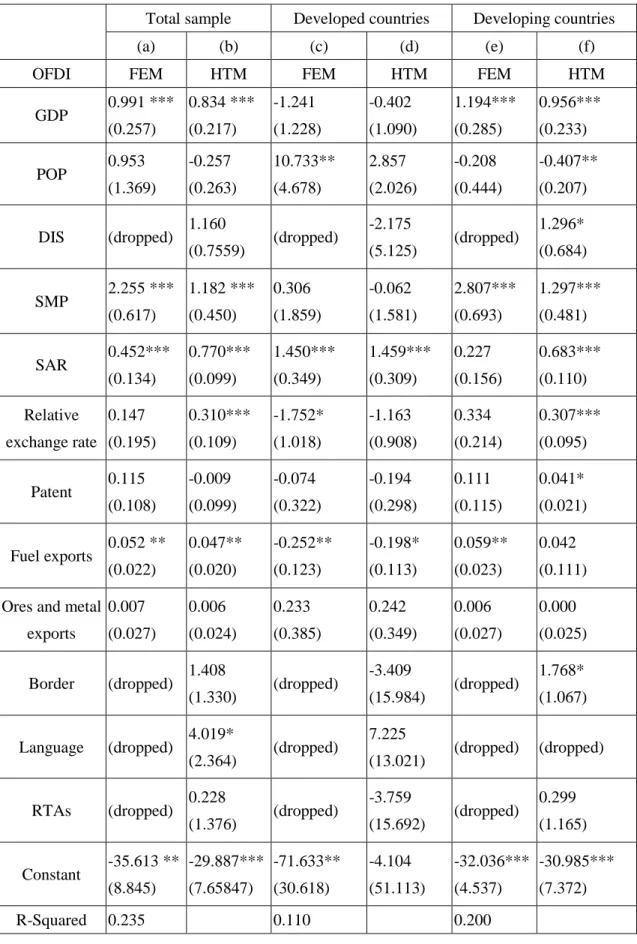
Table 4 displays information regarding the descriptive statistics for the explanatory variables from 2003 to 2009.³Furthermore, Table 4 and Table A (Appendix) reveal that multicollinearity by means of the VIF (variance inflation factors) test (Kutner et al., 2004) and pair-wise correlation between the independent variables are not serious issues in our sample. Table 4 shows that the highest VIF of all variables is 7.62, which is less than ten, although the average VIF of 2.56 is greater than one. On the other hand, as shown in Table A (Appendix), the pairwise correlations coefficients matrix reveals that the dependent variables are not serious

3 Themaximum amountoftheChina’soutwradis US$16,449,894 to Hong Kong, while the minimum number is US$10,000. The top GDP is US$ 14,441 billion for US in 2008, while the lowest GDP is US$ 217 for Togo, in the year 2003. The largest population is 1.15 billion, for India, in 2009, whereas the smallest population is 79 thousand for Antigua and Barbuda in the year 2003. The shortest distance is 962 km from China to Korea, while the longest distance is 19,243 km from China to Argentina. The greatest relative exchange rate is US$4,192 to Iran, while the Kuwait has the lowest degree of relative exchange rate, or US$0.035436. The highest patent number is 102,267 for US in 2006. Russia has the highest fuel exports or US$ 309.7 billion in 2008, while US has the highest ores and metals exports or US$ 53.1 billion in 2008.

(13)

issues in our sample.

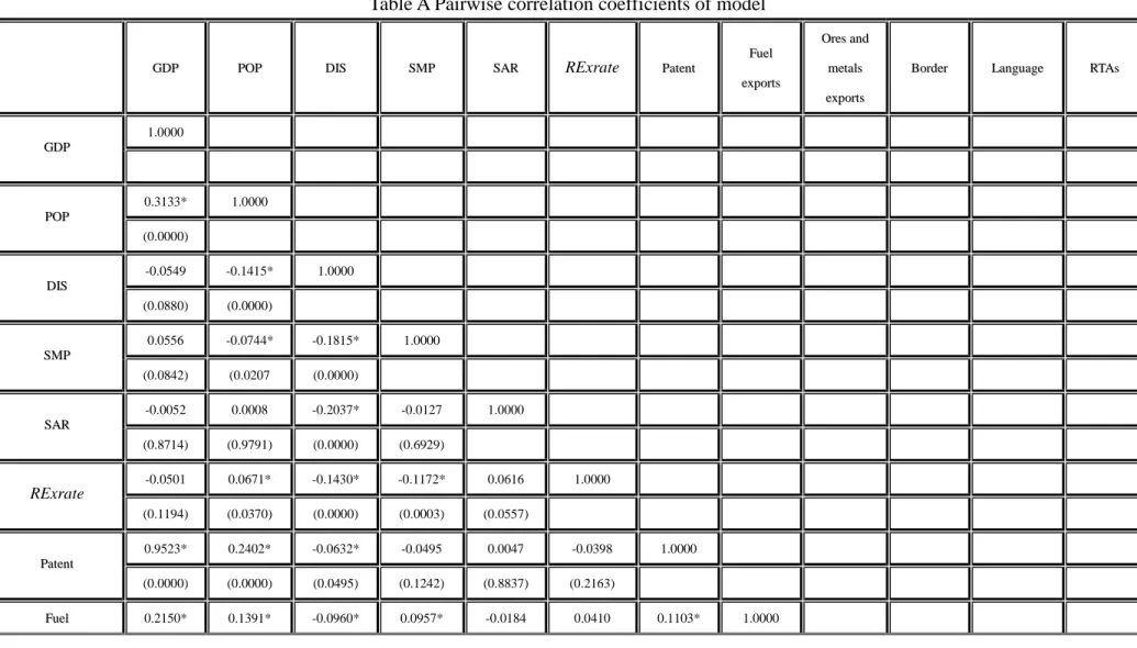
Table 3 An overview of factors determining OFDI

Variables Desciptions Expected sign

Sources (2003-2009) References

Outward FDI (OFDI)

China’sOutward Foreign Direct Investment stock by countries and regions.(US$10 thousands)

Dependent variable

China Minsitry of Commerce,

Statistical Bulletin of China’sOutward Foreign Direct Investment.

Cheng and Ma (2007)

GDGDPP

Gross Domestic Product of country.(US$

millions)

+ International Monetary Fund of World Economic Outlook (WEO) Database

Linnemann (1966)；

Cheng and Ma(2007)；

Blonigen et al.(2007) ； Garretsen and Peeters(2009)

Population (POP)

Population of country. (thousands)

+ U. S. Census Bureau of International Data Base (IDB)

Linnemann (1966) ； Cheng and Ma(2007) ； Blonigen et al.(2007) ； Garretsen and Peeters(2009)

DDiissttaannccee(D(DIISS))

Geographical distance between the capitals of host country and Beijing.(km)

? Timeanddate.com：

Caculate Distance Between Two Locations

Bergstrand (1985) ； Grossman(1998) ； Hummels (1999) ； Stone and Jeon (2000) ； Cheng and Ma(2007) ； Blonigen et al.(2007) ； Garretsen and Peeters(2009)

SuSurrrroouunnddiinngg--MMaa rkrkeettPoPotetennttaaiill

((SSMMPP)) (o(orrRReemmoorreenneessss))

It is measured as the distance-weighted average real gross domestic product of other host countries in the sample.

k j

DIS SMP GDP

k jk

k j







^,

? Head and Mayer (2004) ；

Blonigen et al. (2004, 2007, 2008) ；

Garretsen and Peeters(2009)

(14)

(US$ millions)

SSppaattiiaall--AAuuttoorreeggrr esesssiioonn (S(SAARR))

SASARR captures the proximity of the observed host to other host countries.

(US$10 thousands)

? Coughlin and Segev (2000);

Blonigen et al.(2007);

Garretsen and Peeters(2010)

ReRellaattiivvee eexxcchhaannggeerarattee

((RExrate))

The foreign currency price of one unit of the home currency. And it adjusted by the ratio of the CPI of the host country to the CPI of China.

(US$)

ct jt cjt cjt

CPI Exrate CPI

RExrate

 *

+ The World Bank：

DataBase Online

Cushman (1988) ； Quéré et al. (2001)

P Paatteenntt

It captures the technical standard of the host country.

+ United States Patent and Trademark (USPTO)

Greenwood and Yorukoglu (1997)

F

Fuueellexexppoorrttss ( (FFEE))

Annual fuel exports of host country.

(US$)

+ The World Development Indicators (WDI) OOrreessaannddmemettaallss

exexppoorrttss (O(OMMEE))

Annualoorreessaanndd memettaallsseexxppoortrtss of host country. (US$)

+ The World Development Indicators (WDI)

Makino et al. (2002)

B Boorrddeerr

It is a dummy variable for its sharing a common border with China.

+ The World

Factbook-Languages

Lennon (2006) ； Cheng and Ma(2007)

LLaanngguuaaggee

It is a dummy variable for the use of the chinese language.

+ The World Factbook-Land Boundaries

Veugelers (1991) ； Park (2002) ； Lennon (2006)

RTRTAAss

It is a dummy variable for host

+ The Offical Website of Association of

(15)

country is an

ASEAN’members.

Southeast Asian Nations

Note：“-”denotesthenegativesign；“+”denotesthepositive sign；“?”denotes the indeterminate sign.

Table 4: Summary Statistics and VIF

Variables Mean Standard

Deviation Minimum Maximum VIF

OFDI 64785.13 717288.9 1 1.64E+07 -

GDP 327287.2 1251080 217 1.44E+07 7.62

POP 3589.323 10248.02 7.9 115689.8 3.04

DIS 8510.5 3813.195 962 19243 1.92

RExrate 131.5886 449.7327 0.035436 4192.615 1.73

Patent 1257.909 8611.22 1 102267 3.29

Fuel exports(FE) 1.06E+10 2.74E+10 1.68E-10 3.10E+11 3.08 Ores and metal exports(OME) 3.07E+09 6.97E+09 9.27E-15 5.31E+10 2.76 SMP 9539.478 6477.088 2782.694 42896.53 1.47 SAR 73926.67 311987.5 2144.892 7032440 1.58

Border 0.0942029 0.292262 0 1 1.55

Language 0.0217391 0.145906 0 1 1.22

RTAs 0.0724638 0.259389 0 1 1.40

4.

Empirical Model and Specification Testing

4.1 Empirical Model

We first construct an augmented gravity panel-data model as Equation (1).

cjt cj cjt

cjt X

OFDI 



₁ 







, (1)

where j1,2,...,N , t 1,2,...,T . The vector of X_cjt consists of a set of explanatory variablesrepresenting thedeterminantsofChina’sOFDI (OFDI_cjt) from

China (c) to country j in period t . Basically, X_cjt captures the following both

(16)

keyterms. The first is the host variables (Blonigen et al., 2007; Garretsen and Peeters, 2009) contains the determinating factors of the host countries (GDP, population, distance between China and host contries, skill quality(patent), trading costs (real exchange rate,

ct jt cjt

cjt CPI

Exrate CPI

RExrate  * RExrate_cjt, the foreign currency price of one unit of the home currency, which adjusted by the ratio of the CPI of the host country j and the CPI of China

c at time t free trade agreement), fuel, ores and metal

exports, border and language ). Secondly, the market potential surrounding (SMP) a host country and the spatial effects (spatial-autoregression, SAR) are required to determine third-country effects and Chinese firms’outward FDI motivations in the model.

 is an error term which is distributed i.i.d. across country pairs and over

_cjt

time;



_cj 



_cu_cj,

 is assumed to be a fixed parameter to be estimated and

_c u_cj is an unobservable time-invariant random effect from China

c to country j , and

0

ucj . That is, heteroskedasticity could occur in the regression model and hence a Hausman specification test is required.

Thus, following Equation (1) and the definition of spatial lag model (Blonigen et al., 2007; Garretsen and Peeters, 2009), the corresponding reduced-form augmented gravity model is written as in Equation (2):

       

^,

xrate

11 10

9

8 7

6 5

4 3

2 1

cjt cj jt cjt

cjt jt

jt jt

cjt cjt

jt jt

cjt

RTA a Language a

Border a

SAR n

SMP n OME

n FE

n Patent

n

RE n DIS

n POP

n GDP

n nOFDI















(2)

where SAR_jt W OFDI_jt, the weights matrix

   

⁰ ⁰ ^, ^.

0

, ,

k j i d

w d w

d w d

w

d w d

w W

j k t i k t

k j t i

j t

k i t j i t



















 w_t

 

d_i_,_j denotes the functional form

(17)

of the weights between both host countries iand j .⁴ All varuables are defined in Table 3.

4.2 Specification testing

In choosing the empirical method to be adopted in nine cases (including total sample countries, developed countries, developing countries (Table B, Appendix), petroleum exporting countries and Aferican petroleum exporting countries and four regions (Table C, Appendix)) as shown in Table 5, we consecutively employ the Breusch-Pagan Lagrange Multiplier (BP LM) test, the Hausman test and and the over-identification test of the Hausman-Taylor model (HTM, Hausman and Taylor, 1981) as follows. First, we employ the BP LM test for the autoregression test. If autoregression exists, then we can choose either the full general least squares method (FGLS) or general method of moments (GMM) to conduct a further estimation. If not, the Hausman test is required to check whether the optimal testing method is the random effects model (REM) or fixed effects model (FEM) together with FGLS.

The FEM, however, requires that the invariant explanatory variables be dropped in the fixed transformation (i.e., a common land border, language and RTAs). We follow Egger’s (2002, 2005) and Walsh’s (2008) suggestions, and employ the HTM over-identification test to test the appropriateness of the HTM compared to the FEM.

If we can not reject the null hypothesis that the unobserved effects are correlated with other regressors, then the HTM is more adequate. On the other hand, we have to employ other appropriate estimators as the HTM can not be identified due to collinearity.

Table 5 further reports that the HTM test provides adequate estimators for six

4 wt

 

di_,j 10/dij, while the shortest distance between Congo (Brazzaville) and Congo (Kinshasa) equals to 10 km.

(18)

cases as the FEM has a better fit for the total sample countries, developing countries and Asia-Pacific countries cases.

Table 5 Specification Test Results and Empirical Model Adopted

Regions

Autoregression Test (BP LM test)

Hausman Test

Hausman-Taylor Over-Identification

Test

Empirical Model adopted

Observations

1225.33** 57.22** 30.315**

total sample

(138 countries) (0.0000) (0.0000) (0.0000) FEM 966 108.8** 68.61** 4.648

developed countries (26 countries)

(0.0000) (0.0000)

0.5897 HTM

182

907.43** 60.29** 34.378**

developing countries (112 countries)

(0.0000) (0.0000) (0.0000) FEM

784

petroleum exporting countries (70 countries)

551.55***

(0.0000)

58.61***

(0.0000)

11.24

(0.0813) HTM

490

Aferican petroleum

exporting countries (20 countries)

60.26***

(0.0000)

47.31***

(0.0000)

5.862

(0.4388) HTM

140

409.47** 30.77** 16.136*

Asia-Pacific countries

(46 countries) (0.0000) (0.0002) (0.0130) FEM

322

71.49** 14.91 3.62

Americas

(19 countries) (0.0000) (0.0609) (0.7280) HTM 133

263.53** 16.74* 11.43

African Countries

(44 countries) (0.0000) (0.0330) (0.0760) HTM

308

134.28** 17.96* 3.251

European Countries

(29 countries) (0.0000) (0.0215) (0.7767) HTM

203

* Significant at 10%; ** significant at 5%; *** significant at 1%

Standard errors in parentheses

(19)

5.

Empirical results

The following estimations for a panel of annual data on China’s OFDI into 138 countries or destinations from 2003 to 2009. For further investigating the motivations behind the China’sOFDIin differenttypesofcountries,we disaggregate the data into sub-samples of the deveploed and developing countries or the petroleum exporting countries and Aferican petroleum exporting countries. The last analysis reveals the empirical results by the sub-samples of the Aferican, American, Asia-Pacific and European countries

5.1 Base reults for the global-wide analysis

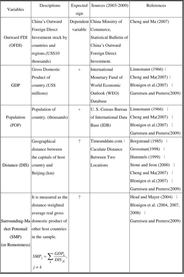
As shown in Table 6, the columns (1) and (2) present FEM and HTM estimates and provide that the host GDP has significantly positiveeffectsto attractChinesefirms’ OFDI⁵ (Blonigen et al.,2007; Cheng and Ma, 2007; Garretsen and Peeters, 2010).

Similar with the findings of Stone and Jeon (2000), distance has no significantly negative impact on the China’s OFDI. The positive coefficients of surrounding-market potential (SMP) and spatial autoregression (third-country effect) (SAR) indicates that China’s OFDI into the world is a complex-vertical (or fragmentation) FDI⁶. The result confirms that distance is not a costly factor to China’s OFDI.

The third key result is that the increasing real exchange rate (i.e., depreciation), which is adjusted by the ratio of the relative CPI of the host country to the CPI of the home country, of the parent country currency vis-à-vis the host country currency

5 Thecoefficientofthe hostGDP in American region to China’sOFDI,2.3338, is the highest than other regions. In words, the home market effect is stongly significant in American countries (Table D, Appendix).

6 We find that a complex-verticalChina’sOFDIplaysakey rolein Asia-Pacific (46 countries), Aferican (44 countries) and European areas (29 countries) while Chinese firms prefer a horizontal OFDI in American region (19 countries) (Table A, and Table D, Appendix).

(20)

increasesChina’sfirms’OFDI. The main reason for this is that China’sOFDI is accounted for in the currency of China (Renminbi, RMB) could be hurt only slightly by the currency depreciation, but the investment accounted for in US dollars could increase instead. This result clearly implies that the China’sOFDI is inelastic to the depreciation of RMB. In words, the China’s currency depreciation strategy is advantageous to the China’sOFDI.

Finally, the fuel exports of host countries significantly strengthensChina’sOFDI, while a common language has a significantly positive impact on Chinese firms’

OFDI consistent with the findings of Park (2002), Lennon (2006) and Cheng and Ma(2007).

5.2. Sub-sample results

Columns (2) and (3) in Table 6 first reveal that the economic size of developing countries significantly attracts China’s OFDI at 1%, while the positive coefficient of SMP gives that the market potential surrounding the host developing countries promotes Chinese firms’OFDI as well. Second, the findings of positive coefficient SAP show that China’s complex-vertical (or fragmentation) OFDI plays an important role in the developed countries. Third, in line with the findings of Makino et al.（2002）,China’sfirmspreferto directly investinto thedeveloping countiresfor fuel rather than ores and metal minerals controls.

China has become top three trading partners of Aferica with the U.S. and France after 2005 (UNCTAD, 2007). By the Standsrd Bank estimations, the total amount of China’s cumulative OFDI in Aferica is about $ 30bn~40bn from the period 2007 to 2009 mainly for manufacturing, natural resources (fuels, minerals, etc.), infrastructure construction and other services (UNCTAD, 2007, 2010; Financial Times, 2010). In

(21)

particular, African countries’raw materialexports(petroleum,and oresand metals)to China accounted for 87% of its total exports in 2010 (Making it, 2011). We further investigate the determinants and motives of Chinese Firms’OFDI in Aferica by sub-samples, Aferican petroleum exporting countries⁷ and petroleum exporting countries.

As shown in Columns (1) in Table 7, for the dummy variable, the Aferica has a significantly positive contribution in terms of enhancing China’sOFDI in Aferican region for various motives, which is consistent with the realities mentioned above.

Columns (2) and (3) in Table 7 further show that the host GDP of petroleum exporting countries and Aferican petroleum exporting countries has a strong positive and significant coefficient at 1% (an elasticity of 1.0946 and 2.0869, respectively).

The significant positive coefficient of surrounding-market potiential implies an export-platform China’s OFDI occured in Aferican petroleum exporting countries and petroleum exporting countries. In words, China’s firms are likely to serve the surrounding markets through exports using the host plarform.

The increasing real exchange rate increases (depreciation) China’sfirms’OFDI into Aferican petroleum exporting countries and petroleum exporting countries (an elasticity of 1.5376 and 0.6387 respectively) which plays the same role with those of full sample case⁸. The positive coefficient of fuel exports reveals that the greater the fuel exports of the host (Aferican) petroleum exporting countries, the greater the China’sOFDI. Therefore, we can conclude that fuel extraction motives significantly promoteChina’sOFDI into the host (Aferican) pletroleum exporting countries.

7 Thecoefficientoffuelexportsto China’sOFDIisalso significantin Aferican 44 countriesin disaggregrated case in Table D, Appendix.

8 The increasing real exchange rate promotes China’s OFDI in Aferican 44 countries as well (Table D, Appendix).

(22)

Table 6 Total sample, developed and developing sub-samples results

Total sample Developed countries Developing countries

(a) (b) (c) (d) (e) (f)

OFDI FEM HTM FEM HTM FEM HTM

GDP 0.991 ***

(0.257)

0.834 ***

(0.217)

-1.241 (1.228)

-0.402 (1.090)

1.194***

(0.285)

0.956***

(0.233) POP 0.953

(1.369)

-0.257 (0.263)

10.733**

(4.678)

2.857 (2.026)

-0.208 (0.444)

-0.407**

(0.207) DIS (dropped) 1.160

(0.7559) (dropped) -2.175

(5.125) (dropped) 1.296*

(0.684)

SMP 2.255 ***

(0.617)

1.182 ***

(0.450)

0.306 (1.859)

-0.062 (1.581)

2.807***

(0.693)

1.297***

(0.481)

SAR 0.452***

(0.134)

0.770***

(0.099)

1.450***

(0.349)

1.459***

(0.309)

0.227 (0.156)

0.683***

(0.110) Relative

exchange rate 0.147 (0.195)

0.310***

(0.109)

-1.752*

(1.018)

-1.163 (0.908)

0.334 (0.214)

0.307***

(0.095)

Patent 0.115 (0.108)

-0.009 (0.099)

-0.074 (0.322)

-0.194 (0.298)

0.111 (0.115)

0.041*

(0.021)

Fuel exports 0.052 **

(0.022)

0.047**

(0.020)

-0.252**

(0.123)

-0.198*

(0.113)

0.059**

(0.023)

0.042 (0.111) Ores and metal

exports

0.007 (0.027)

0.006 (0.024)

0.233 (0.385)

0.242 (0.349)

0.006 (0.027)

0.000 (0.025)

Border (dropped) 1.408

(1.330) (dropped) -3.409

(15.984) (dropped) 1.768*

(1.067)

Language (dropped) 4.019*

(2.364) (dropped) 7.225

(13.021) (dropped) (dropped)

RTAs (dropped) 0.228

(1.376) (dropped) -3.759

(15.692) (dropped) 0.299 (1.165)

Constant -35.613 **

(8.845)

-29.887***

(7.65847)

-71.633**

(30.618)

-4.104 (51.113)

-32.036***

(4.537)

-30.985***

(7.372)

R-Squared 0.235 0.110 0.200

(23)

Number of

Observation 966 966 182 182 784 784

“－”denotes variable excluded

Table 7 The empirical results of full sample added dummy variable and Sub-samples by petroleum exporting

Full sample added dummy variable with Aferica

Petroleum exporting

countries

Aferican petroleum

exporting countries

Outward FDI FEM HTM HTM HTM

GDP 0.9907***

(0.2577)

0.9641***

(0.2246)

1.0946***

(0.2740)

2.0869***

(0.4231)

POP 0.9534

(1.3695)

-0.3878 (0.2635)

-0.5392 (0.5105)

-1.4424**

(0.6685)

DIS (dropped) 0.4923

(0.7591)

0.9831 (2.1617)

-7.9047 (8.0095) SMP 2.2545***

(0.6174)

0.9932**

(0.4438)

2.7977***

(0.7040)

2.0412**

(1.1670) SAR 0.4528***

(0.1343)

0.7885***

(0.0978)

0.2249 (0.1532)

-0.1378 (0.2578)

Relative exchange rate

0.1470 (0.1956)

0.2181**

(0.1100)

0.6387***

(0.1886)

1.5376***

(0.3147)

Patent 0.1157 (0.1084)

0.0167 (0.1001)

0.0681 (0.1285)

0.3386 (0.2823)

Fuel exports 0.0524**

(0.0225)

0.0475**

(0.0205)

0.1399***

(0.0336)

0.1780***

(0.0341)

Ores and metal exports

0.0067 (0.0271)

0.0049 (0.0248)

0.0126 (0.0264)

0.0439 (0.0915)

Border (dropped) 1.8868

(1.2888)

1.3571

(3.2038) －

Language (dropped) 3.2868 (2.2707)

0.2132

(3.0703) －

ASEAN (dropped) 0.5773

(1.3192) －－

(24)

Africa

dummy (dropped) 2.1832**

(0.8771) －－

Constant -35.6129***

(8.8453)

-23.5390***

(7.6628)

-40.2701**

(20.2882)

45.8188 (75.3976)

“－”denotes variable excluded

5. Conclusion remarks

The present study characterizes the patterns and investigates the determinants of theChina’sOFDIinto 138 countriesforthe2003-2009 period. The trade magnitude and pattern of Chinese OFDI typically indicates two main summaried characteristics.

One is that no-financial OFDI plays an important role while Hong Knog, Cayman Islands and British Virgin Islands are top three outflow regions. The second characteristicisthatChina’sOFDInotonly focuseson high-tech or high-intensive industries in developed countries but also approaches to natural resources extraction on developed and developing countries such as Aferican countries, Australia and Kazakhstan,etc., which matches with Rosen and Hanemann’s(2011)findings.

To choose appropriate testing models, we first employ the Breusch-Pagan LM test, the Hausman test and the Hausman-Taylor over-identification test to find the appropriate empirical method for nine cases, even though HTM has been used by scholars to estimate the gravity model for trade in goods and services in recent years.

The consequences of specification testing indeed support the view that the HTM or FEM can be appropriated with respect to the corresponding cases.

The empirical results for investigating the determinants of China’s OFDIare summarized as follows. First, from the perspective of a global-wide analysis, host economic size (GDP) has significant positive effects in terms of promoting Chinese

(25)

investment outflows but distance does not have significantly negative impact to China’s OFDI. The second key empirical result is that the magnitude of Chinese OFDI is due to complex-vertical investment while Chinese firms prefer to the market potential surrounding the host developing countries from the coefficients of surrounding market potential and spatial autogression simultaneously. Third, the China’s OFDI is inelastic to the depreciation of the currency of China, RMB. Fourth, in line with the findings of Park (2002), Lennon (2006) and Cheng and Ma (2007), a common language has a positive impact in relation to China’s OFDI. Fifth, the fuel exports of host countries promote China’s OFDI.

Six, Chinese firms prefer an export-platform FDI for the petroleum exporting countries and Aferican petroleum exporting countries. Finally, the empirical results revealthatfuleextraction moviesstrengthen China’sOFDIinto thehost(Aferican) petroleum exporting countries consistent with the realities of Chinese firms’OFDI strategies in the last ten years. Consequently, we believe that more disaggrgated data should serve as a useful direction for research in further studies, although our results provide a quite complete analysis of the China’sOFDIin recent years.

(26)

Appendix

Table A Pairwise correlation coefficients of model

G

GDDPP POPOPP DDIISS SSMMPP SSAARR RExrate PaPatteenntt

FFuueell

eexxppoorrttss O Orreessanandd

m meettaallss

e exxppoorrttss

B

Boorrddeerr LaLanngguuaaggee RRTTAAss

1.0000 G

GDDPP

0.3133* 1.0000 PPOOPP

(0.0000)

-0.0549 -0.1415* 1.0000 DIDISS

(0.0880) (0.0000)

0.0556 -0.0744* -0.1815* 1.0000

SSMMPP

(0.0842) (0.0207 (0.0000)

-0.0052 0.0008 -0.2037* -0.0127 1.0000

SASARR

(0.8714) (0.9791) (0.0000) (0.6929)

-0.0501 0.0671* -0.1430* -0.1172* 0.0616 1.0000

RExrate

(0.1194) (0.0370) (0.0000) (0.0003) (0.0557)

0.9523* 0.2402* -0.0632* -0.0495 0.0047 -0.0398 1.0000

P Paatteenntt

(0.0000) (0.0000) (0.0495) (0.1242) (0.8837) (0.2163)

F

Fuueell 0.2150* 0.1391* -0.0960* 0.0957* -0.0184 0.0410 0.1103* 1.0000

(27)

e

exxppoorrttss (0.0000) (0.0000) (0.0028) (0.0029) (0.5680) (0.2035) (0.0006)

0.5978* 0.2451* 0.0492 0.1331* -0.0157 -0.0432 0.4578* 0.3630* 1.0000

O Orreessaanndd

m

meettaallssexexppoorrttss (0.0000) (0.0000) (0.1261 (0.0000) (0.6259) (0.1802) (0.0000) (0.0000)

-0.0397 0.2850* -0.4374* -0.0768* 0.2651* (0.2192* -0.0448 0.0791* -0.0161 1.0000

BoBorrddeerr

(0.2172) (0.0000) (0.0000) (0.0170) (0.0000) (0.0000) (0.1639) (0.0139) (0.6178)

-0.0252 -0.0465 -0.2233* -0.0452 0.4631* -0.0426 -0.0152 0.0170 0.0607 0.1220* 1.0000

Language

(0.4338) (0.1491) (0.0000) (0.1600) (0.0000) (0.1855) (0.6360) (0.5986) (0.0593) (0.0001)

-0.0482 0.0589 -0.3629* -0.1469* 0.1104* 0.4064* -0.0387 0.0008 -0.0472 0.1969* 0.1500* 1.0000

TRAs

(0.1343) (0.0673) (0.0000) (0.0000) (0.0006) (0.0000) (0.2297) (0.9791) (0.1428) (0.0000) (0.0000)

*denotes the significance level at 5%; ( ) denotes P-Value.

(28)

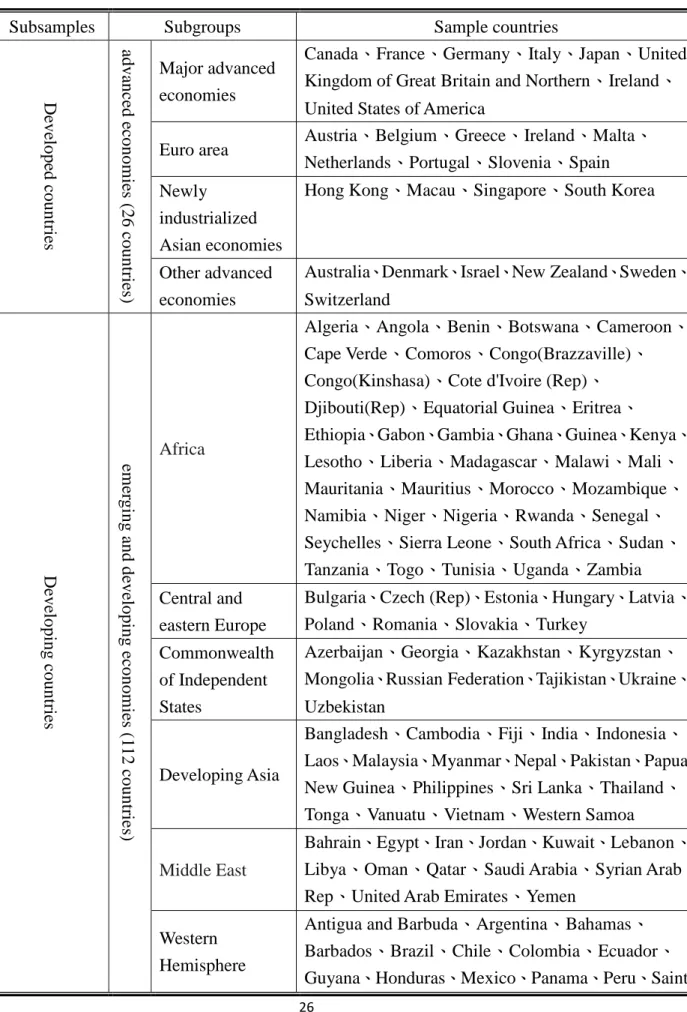
Table B Subsamples by the degree of development

Subsamples Subgroups Sample countries

Major advanced economies

Canada、France、Germany、Italy、Japan、United Kingdom of Great Britain and Northern、Ireland、

United States of America

Euro area Austria、Belgium、Greece、Ireland、Malta、

Netherlands、Portugal、Slovenia、Spain Newly

industrialized Asian economies

Hong Kong、Macau、Singapore、South Korea Developedcountries advancedeconomies(26countries) Other advanced

economies

Australia、Denmark、Israel、New Zealand、Sweden、

Switzerland

Africa

Algeria、Angola、Benin、Botswana、Cameroon、

Cape Verde、Comoros、Congo(Brazzaville)、

Congo(Kinshasa)、Cote d'Ivoire (Rep)、

Djibouti(Rep)、Equatorial Guinea、Eritrea、

Ethiopia、Gabon、Gambia、Ghana、Guinea、Kenya、

Lesotho、Liberia、Madagascar、Malawi、Mali、

Mauritania、Mauritius、Morocco、Mozambique、

Namibia、Niger、Nigeria、Rwanda、Senegal、

Seychelles、Sierra Leone、South Africa、Sudan、

Tanzania、Togo、Tunisia、Uganda、Zambia Central and

eastern Europe

Bulgaria、Czech (Rep)、Estonia、Hungary、Latvia、

Poland、Romania、Slovakia、Turkey Commonwealth

of Independent States

Azerbaijan、Georgia、Kazakhstan、Kyrgyzstan、

Mongolia、Russian Federation、Tajikistan、Ukraine、

Uzbekistan

Developing Asia

Bangladesh、Cambodia、Fiji、India、Indonesia、

Laos、Malaysia、Myanmar、Nepal、Pakistan、Papua New Guinea、Philippines、Sri Lanka、Thailand、

Tonga、Vanuatu、Vietnam、Western Samoa

Middle East

Bahrain、Egypt、Iran、Jordan、Kuwait、Lebanon、

Libya、Oman、Qatar、Saudi Arabia、Syrian Arab Rep、United Arab Emirates、Yemen

Developingcountries emerginganddevelopingeconomies(112countries)

Western Hemisphere

Antigua and Barbuda、Argentina、Bahamas、

Barbados、Brazil、Chile、Colombia、Ecuador、

Guyana、Honduras、Mexico、Panama、Peru、Saint

(29)

Vincent and the Grenadines、Suriname、Uruguay、

Venezuela

Note︰

1. On July 1,1997,Hong Kong wasreturned to thePeople’sRepublicofChinaand becameaSpecial Administrative Region of China.

2. Mongolia, which is not a member of the Commonwealth of Independent States, is included in this group for reasons of geography and similarities in economic structure.

3. A few countries are currently not included in these groups, either because they are not IMF members and their economies are not monitored by the IMF or because databases have not yet been fully developed. Because of data limitations, group composites do not reflect the following countries: the Islamic Republic of Afghanistan, Bosnia and Herzegovina, Brunei Timor-Leste.

Sources：World Economic Outlook, International Monetary Fund (April 2008)

Table C Subsamples by continent

Subsamples Sample countries

Asia Pacific (46 countries)

Afghanistan、Australia、Bahrain、Bangladesh、Brunei、

Cambodia、East Timor、Fiji、Hong Kong、India、Indonesia、

Iran、Israel、Japan、Jordan、Kazakhstan、Kuwait、Kyrgyzstan、

Laos、Lebanon、Macau、Malaysia、Mongolia、Myanmar、Nepal、

New Zealand、Oman、Pakistan、Papua New Guinea、Philippines、

Qatar、Saudi Arabia、Singapore、South Korea、Sri Lanka、Syrian Arab Rep、Tajikistan、Thailand、Tonga、Turkey、United Arab Emirates、Uzbekistan、Vanuatu、Vietnam、Western Samoa、Yemen The Americas

(19 countries)

Antigua and Barbuda、Argentina、Bahamas、Barbados、Brazil、

Canada、Chile、Colombia、Ecuador、Guyana、Honduras、Mexico、

Panama、Peru、Saint Vincent and the Grenadines、Suriname、

United States of America、Uruguay、Venezuela Africa

(44 countries)

Algeria、Angola、Benin、Botswana、Cameroon、Cape Verde、

Comoros、Congo(Brazzaville)、Congo(Kinshasa)、Cote d'Ivoire (Rep)、Djibouti(Rep)、Egypt、Equatorial Guinea、Eritrea、

Ethiopia、Gabon、Gambia、Ghana、Guinea、Kenya、Lesotho、

Liberia、Libya、Madagascar、Malawi、Mali、Mauritania、

Mauritius、Morocco、Mozambique、Namibia、Niger、Nigeria、

Rwanda、Senegal、Seychelles、Sierra Leone、South Africa、