沉浸邊界法在囊泡問題之數值模擬

國立交通大學

應用數學系

博士論文

 

沉浸邊界法在囊泡問題之數值模擬

 

Immersed Boundary Methods for Simulating

Vesicle Dynamics

                   

研 究 生

 

：

 

胡偉帆

指 導 教 授

 

：

 

賴明治 教授

 

沉浸邊界法在囊泡問題之數值模擬

Immersed boundary methods for simulating vesicle dynamics

研 究 生：胡偉帆

Student：Wei-Fan Hu

指導教授：賴明治 教授

Advisor：Ming-Chih Lai

國 立 交 通 大 學

應 用 數 學 系

博 士 論 文

A Dissertation

Submitted to Department of Applied Mathematics National Chiao Tung University

in partial Fulfillment of the Requirements for the Degree of

Doctor of Philosophy in

Applied Mathematics

July 2014

沉 浸 邊 界 法 在 囊 泡 問 題 之 數 值 模 擬

研究生：胡偉帆

指導教授

：

賴明治

教授

國立交通大學

應用數學系 博士班

摘

要

過去數十年來，囊泡問題的動態數值問題一直是個熱門的議題。在本論文中，

我們透過沉浸邊界法 (immersed boundary method)來描述囊泡的流體數學模型，

公式，包含 Eulerian 座標系下的流體方程式以及建立在 Lagrangian 座標系中有關

界面的變數，而這兩個座標系之間各個變數的轉換，則是藉由 Dirac delta function

來連結。本論文致力於發展簡易且精確的數值方法來模擬此流體界面問題。

首先，我們提出了一個 fractional step immersed boundary method 用於模擬不

可延展界面之問題(不考慮 bending effect)。我們證明了作用在表面張力 spreading

operator 是 surface divergence operator 的斜自伴算子 (skew-adjoint)。利用這個特

性，對於流體變數之離散我們可獲得一個對稱矩陣，並可使用 fractional step 方法

解決此線性系統。我們比較了此數值方法的精確度，以及利用本方法研讀不可延

展界面在 shear flow 底下之數值模擬。

再來我們研發出一種 unconditionally stable immersed boundary method 作為二

維的囊泡在 Navier-Stokes 流體之模擬。我們用一種半隱示 (semi-implicit)的方法

來表示囊泡之界面力，而與介面力相關的 stretching factor 則可透過其他的方程式

獲得。我們證明出在本方法中，流體系統的總能量將隨時間而遞減。另外，利用

projection method，對於流場我們推導出一個對稱正定的線性系統，此矩陣可利

用多重網格法 (multi-grid method)有效率地計算其解。在數值實驗中，我們驗證

本方法之精準度，並在效率上遠勝於傳統之顯示邊界力處裡方法。同樣我們也利

用本方法研讀囊泡在二維座標底下之型變動態系統。

最後，我們延伸至三維軸對稱的囊泡問題。與其將表面張力作為一 Lagrange's

multiplier 來迫使囊泡之不可延展性，我們定義一種 spring-like 表面張力作為本模

型之逼近。囊泡的邊界可利用 Fourier spectral 方法來表示，並且我們可精準地計

算出界面上的平均曲率、高斯曲率等等。透過一系列之數值模擬，我們展示出本

方法之應用性與可靠性。我們使用本方法研讀囊泡在靜止流、重力場影響及

Poiseuille flow 下之動態型變問題。

誌

謝

很幸運的我終於畢業了，說到寫致謝文這檔事每次都讓我頭痛不已，特別不想寫些似流 水帳類的文章。不過自詡小文青的我，真正撰寫時，卻突然變得好像失憶般地不知道該寫些什 麼了。 當然我不會忘記首先該感謝的人是我的指導教授賴明治大教授，遙想起還在頭髮茂密的碩士班 年代，懵懂無知的我修了一堂賴老大開的應用數學課程，當時真覺得原來我所學的數學可以這 麼好玩、這麼應用，於是乎在抉擇研究領域上自然往應用數學靠上不少。對於把數值計算跟程 式撰寫完全留在大學的我一開始是很慌張的，只好每天跑到系上的圖書館埋頭苦幹（兼吹冷 氣），當我靠自己的能力漸漸補足科學計算的基本常識後終於能開始做些研究，這種滿足感是 我在人生中少有的。當然，在研究的過程中痛苦時常是大於收穫的，也不知怎麼的，我好像愛 上了這種痛苦，不，應該說愛上解決痛苦問題後的收穫吧，我便毅然決然選擇學術圈作為我往 後吃飯糊口的地方。 在賴老大的耳濡目染下，我逐漸地能夠掌握到研究正確的方向 （雖然常常有時候偷懶想 跳過某些步驟時都一定會被抓包，一次次的被修理中我也慢慢地建立做學問該有的嚴謹態 度）。從一開始的在台上演講給寥寥無幾個同學都會雙腿發抖的我，到現在可以從容自在地回 應聽眾的問題，這種經驗可說是非常難得可貴的。我很享受在這種被訓練及磨練下能夠逐漸成 為一個獨立思考的個體，甚至廢寢忘食也只為了解決某個研究上遇到的問題（記得我的第二篇 文章主要的概念還是在夢中想到的）。關於感謝賴老大的詞我想也不必多想了，努力工作吧！ 在四年半的修業過程中，我得感謝許多系上的老師們。依稀記得來到交大第一堂課程就是林琦 焜老師的偏微分方程，著實給我了個震撼教育（不只在數學方面，在個人方面特別要教導我們 該擺脫過往的洗腦教育，關心社會以及土地）。也感謝蔡武廷老師（現任台大）讓我對於流體 方程從零開始建立基礎，幽默逗趣的上課過程讓學習更輕鬆（我記得蔡老師很喜歡用一個詞－ 機車）。當然我必須感謝一起合作的老師們，特別謝謝林文偉老師幫助我解決困難的矩陣問題， 讓我的第一篇論文得以發表。感謝我的口試委員老師們，對本論文的指教及提供了許多有關接 下來要作的研究的意見。 千里馬計畫是我人生中一個很特別的經驗，本來一直認為自己會到美國東岸或西岸去， 沒想到最後到了法國南邊的一個小鎮。在法文只能出口幾句日常問好的狀況下我學習獨立生

活，但也見識到歐洲人是如何熱愛自己的生命（工作時間為早上十點至下午五點，中午還要喝 個二小時的咖啡），快速且全面的文化衝擊讓我見識到世界的廣大。我要感謝傅立葉大學物理 系的 Misbah 教授，在他的熱情招待下我有個舒適的環境能夠安身立命做研究，也讓我見識到 了物理學家們頗析問題的方法及精闢。在法國我認識了交大的學姊 Sharon，不但人美心地善 良也很熱心，幫助我在異鄉搞定許多的生活大小事，就好像我另一個親姊。 最後我要感謝我的家人以及多年來陪伴的好朋友們。謝謝我的父母永遠當我的依靠，長久以來 包容我的懶散、沒耐心。感謝我親愛的朋友們 Howard、仲尹、Nelson、Jeny、麻將、曾鈺傑、 縉祥、叮叮等等，時常一起打球出門玩樂、分享喜怒哀樂的夥伴們。最後我一定要說是何等的 幸運，能夠在交大遇到我女朋友，謝謝妳時常帶給我歡笑，讓我能精力飽滿的度過每一天。

Acknowledgment

First of all, I give an immense gratitude to my advisor, Professor Ming-Chih Lai, who has given me invaluable insights, advices and encouragements. His great knowledge, infinite ideas stimulate me to immerse myself in research and lead me to dig more potential from my brain. Choosing him as my advisor is the best decision I have made, I always believe that all the time. I am not sure that I am capable of showing my gratefulness in words, but I guess the best way to express my thanks is - working hard for him.

I would like to express my gratitude to all the professors whom I took classes from at NCTU, and special thanks to Professor C. K. Lin, who has broadened my view not only extracting knowledge in mathematics but also paying more attention for the politics and our homeland. I extend my thanks to Professor Chaouqi Misbah for hosting me in Joseph Fourier University in Grenoble, also I want to thank friends who made my life colorful in France (Sharon, Nicola, Yara and Zaiyi). Thanks for the supports from Ministry of Science and Technology of Taiwan. In addition, I appreciate the defense committees for their stimulating questions and helpful suggestions to complete this dissertation.

Next I want to express my thanks to Howard (maybe I should call him professor Tseng) and Ken, you two always give me a lot of suggestions not merely in researching but in my life. Thank you my brothers. I also want to thank each person I met in NCTU and all my dear friends, Nelson, Jeny, Yu-Jei, Chin-Hsiang, DingDing etc.

Finally, I deeply appreciate my family, my parents and my sister. They always hold my back and give me endless supports. Thanks for your accompanies and let me get through the hardest time in my life. I left my last thank to my girlfriend YY Lu, who makes me happy and enrich my life everyday, and I believe happiness is the best method for doing research, thank you.

Abstract

Numerical simulation of vesicle dynamics has been a popular issue for many decades. In this dissertation, a mathematical formulation for suspension of vesicle in fluid is modeled by immersed boundary method, where a mixture of Eulerian fluid variables and curve-linear Lagrangian interfacial variables are used, and the linkage between these two variables is a smoothed Dirac delta function. The purpose of this disser-tation is to develop accurate and efficient numerical schemes for simulating vesicle dynamics through immersed boundary method.

Firstly, we propose a fractional step immersed boundary method to mimic dynam-ical system of an inextensible interface (vesicle without bending effect). In addition to solving for the fluid variables such as the velocity and pressure, the present problem involves finding an extra unknown elastic tension such that the surface divergence of the velocity is zero along the interface. By taking advantage of skew-adjoint prop-erty between force spreading operator and surface divergence operator, the resultant linear system of equations is symmetric and can be solved by fractional steps so that only fast Poisson solvers are involved. The convergent tests for present fluid solver is performed and confirm the desired accuracy. The tank-treading motion for an in-extensible interface under a simple shear flow has been studied extensively, and the results are in good agreement with those obtained in literature. This part of work has been published in SIAM Journal of Scientific Computing as in [37].

Secondly, we develop an unconditionally stable immersed boundary method to simulate 2D vesicle under a Navier-Stokes flow. We adopt a semi-implicit bound-ary forcing approach, where the stretching factor used in the forcing term can be computed from the derived evolutional equation. By using the projection method to solve the fluid equations, the pressure is decoupled and we have a symmetric positive definite system that can be solved efficiently. The method can be shown to be un-conditionally stable, in the sense that the total energy of fluid system is decreasing. A resulting modification benefits from this improved numerical stability, as the time step size can be significantly increased. The numerical result shows the severe time step restriction in an explicit boundary forcing scheme is avoided by present method. The part of work has been published in East Asian Journal of Applied Mathematics as in [22].

in a Navier-Stokes flow. Instead of introducing a Lagrange’s multiplier to enforce the vesicle inextensibility constraint, we modify the model by adopting a spring-like tension to make the vesicle boundary nearly inextensible so that solving for the unknown tension can be avoided. We also derive a new elastic force from the modified vesicle energy and obtain exactly the same form as the originally unmodified one. In order to represent the vesicle boundary, we use Fourier spectral approximation so we can compute the geometrical quantities on the interface more accurately. A series of numerical tests on the present schemes have been conducted to illustrate the applicability and reliability of the method. We perform the convergence check for fluid variables for present schemes. Then we study the vesicle dynamics in quiescent flow, Poiseuille and under influence of gravity in detail. The numerical results are shown to be in good agreement with those obtained in literature. The part of work has been published in Journal of Computational Physics as in [23].

Contents

1 Introduction 1

1.1 Blood flow and vesicles . . . 1

1.2 Existing works . . . 3

1.3 Immersed boundary method . . . 3

1.4 Contribution of the present work . . . 4

2 Mathematical model of vesicle hydrodynamics 6 2.1 Vesicle mechanics . . . 6

2.2 Interfacial forces on vesicle . . . 8

2.2.1 In two dimensions . . . 8 2.2.2 In three dimensions . . . 10 2.3 Inextensible formulation . . . 11 2.3.1 In two dimensions . . . 11 2.3.2 In three dimensions . . . 11 2.4 Hydrodynamical equations . . . 12

2.4.1 Incompressible Navier-Stokes equations . . . 12

2.4.2 Coupling the fluid equations to vesicle forces . . . 14

3 Immersed boundary method 16 3.1 Connection between fluids and interfaces . . . 16

3.2 Discrete delta function . . . 17

3.3 Numerical setup . . . 20

3.3.1 Staggered grid . . . 20

3.3.2 Ghost values from boundary conditions . . . 22

3.3.3 Lagrangian manners . . . 24

4 Fractional step immersed boundary method 26 4.1 Governing equations . . . 26

4.2 Numerical algorithm . . . 29

4.3 Implementation details . . . 30

4.3.1 Discrete skew-adjoint operators . . . 30

4.3.3 Fractional step method . . . 32

4.4 Numerical results . . . 34

4.4.1 Convergence and efficiency tests . . . 34

4.4.2 Convergence test for an inextensible interface . . . 36

4.4.3 Tank-treading motion under shear flow . . . 37

5 Unconditionally energy stable immersed boundary method 41 5.1 Governing equations . . . 42

5.2 Numerical algorithm . . . 42

5.3 Energy stability analysis . . . 44

5.4 Modified projection method . . . 47

5.5 Applications to simulating vesicle dynamics . . . 48

5.6 Numerical results . . . 49

5.6.1 Convergence study . . . 49

5.6.2 Maximal time step comparison . . . 50

5.6.3 Tank-treading motion under shear flow . . . 51

6 Simulating three-dimensional axisymmetric vesicles 53 6.1 Governing equations . . . 54

6.1.1 Vesicle boundary forces in axisymmetric coordinate . . . 55

6.1.2 Nearly inextensible approach . . . 57

6.1.3 Elastic boundary force . . . 57

6.2 Numerical discretization . . . 58

6.2.1 Fourier representation of the interface and computation of ge-ometrical quantities . . . 58

6.2.2 Time-stepping scheme . . . 60

6.3 Numerical results . . . 61

6.3.1 Accuracy check for the interfacial geometrical quantities . . . 62

6.3.2 Study on different stiffness number σ0 . . . 63

6.3.3 Convergence test . . . 65

6.3.4 A suspended vesicle in quiescent flow . . . 66

6.3.5 Vesicles under the gravity . . . 66

6.3.6 Vesicles in Poiseuille flow . . . 68

7 Conclusions and future works 73 A Geometrical operators and quantities on a surface 80 B Discrete skew-adjoint operators 81 C Unconditionally stable IB method 82 D Geometrical differential operators in axisymmetric coordinate 84

List of Tables

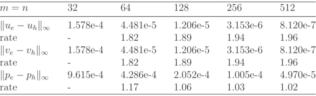
4.1 Numerical accuracy of Stokes solver. . . 35

4.2 The cost of CPU time and iterations. . . 35

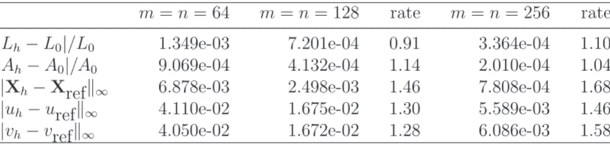
4.3 The mesh refinement results for the perimeter of the interface Lh, the

enclosed area Ah, the interface configuration Xh, and the velocity uh

and vh. . . 37

5.1 The mesh refinement results for the vesicle area Ah, the vesicle

perime-ter Lh, the boundary configuration Xh, and the velocity uh and vh. . 50

5.2 Maximum time steps for the explicit(EP), modified BE and CN schemes with different elastic coefficients σ0. . . 51

5.3 The average CPU time (in seconds) of each time step for different schemes. The total time with ”*” means the estimated value. . . 51

6.1 The mesh refinement study for the computations of H, K and ∆sH by

the spectral method. The maximum absolute error is defined as kH −

Hek∞, where He is exact value of mean curvature. Similar notations

for other quantities. . . 63

6.2 The mesh refinement study for the computations of H, K and ∆sH

by the second-order finite difference method. Only the results of the oscillatory surface are listed. . . 64

6.3 The errors of the area dilating factor, the total surface area, and the volume. . . 64

6.4 The mesh refinement results for the surface area Ah, the enclosed

List of Figures

1.1 The cells in blood. From left to right: red blood cell, platelet and white blood cell. . . 2

1.2 A cartoon showing major proteins on the membrane of RBC. . . 2

2.1 A cartoon showing a vesicle and its molecular structure on membrane. Picture is taken from the web site of Wikipedia. . . 7

2.2 Biconcave equilibrium state of vesicles. . . 7

3.1 The figure of discrete function φi(i = 1, 2, 3, 4) and correspond smoothed

functions φ∗

i (i = 1, 2, 3, 4). . . . 20

3.2 The layout of staggered grid in two-dimensional rectangular domain. The red dots indicate location of pressure p, while the green and blue triangles represent for velocity component u and v respectively. . . . . 21

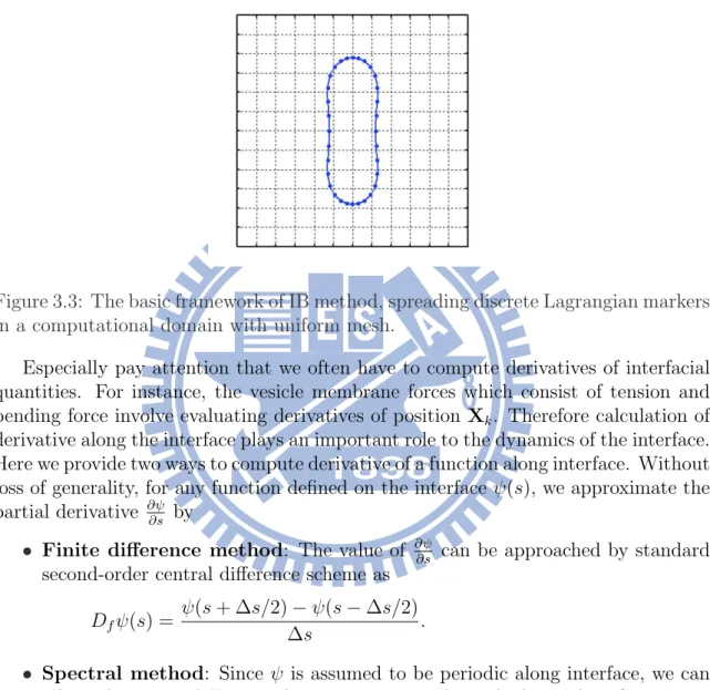
3.3 The basic framework of IB method, spreading discrete Lagrangian markers in a computational domain with uniform mesh. . . 24

4.1 A diagram of an inextensible interface in a shear flow. . . 36

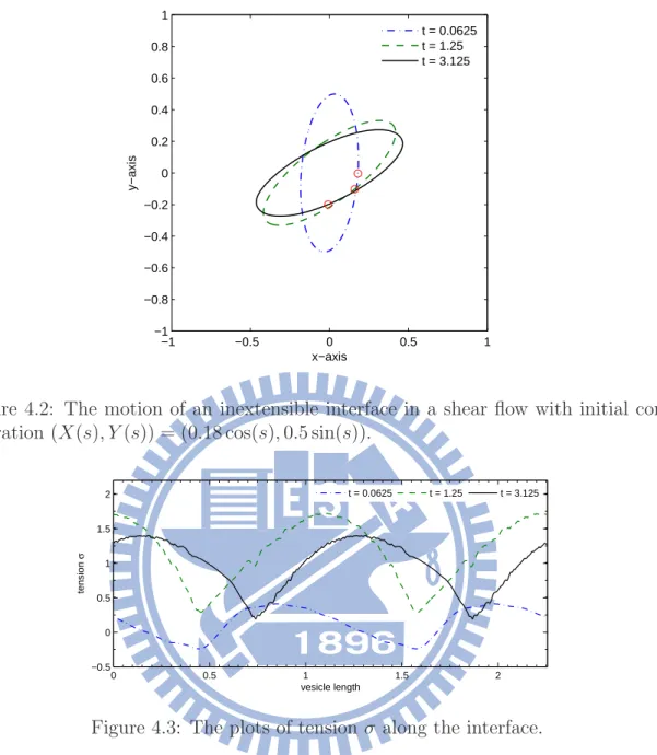
4.2 The motion of an inextensible interface in a shear flow with initial configuration (X(s), Y (s)) = (0.18 cos(s), 0.5 sin(s)). . . . 38

4.3 The plots of tension σ along the interface. . . . 38

4.4 The tank-treading motion of an inextensible interface under a shear flow. 39

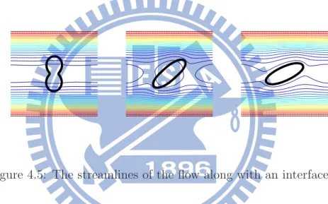
4.5 The streamlines of the flow along with an interface. . . 39

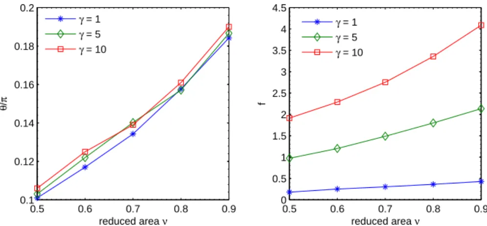
4.6 The inclination angles θ/π (left) and the tank-treading frequency f = 2π±R_{Γu · τ . . . .}dl 40

5.1 The tank-treading motion of a vesicle under shear flow. . . 52

5.2 The inclination angles θ/π (left) and the tank-treading frequency f = 2π±R_{Γu · τ (right) versus reduced areas ν with different shear rates}dl for the tank-treading motion of an inextensible vesicle in a shear flow. 52

6.1 Four different surfaces: Spherical, Prolate, Oscillatory and Peanut-like surface (from left to right). . . 62

6.2 (a) A freely suspended vesicle with different stiffness numbers σ0. σ0 =

2 × 103_{: ’-’; σ}

0 = 2 × 104: ’×’; σ0 = 2 × 105: ’·’. (b) The corresponding

time evolutions of total energy. . . 65

6.3 (a) Snapshots of a freely suspended vesicle in quiescent flow. (b) The corresponding plots result in 3D view. . . 67

6.4 The membrane energy evolution of the freely suspended vesicle. . . . 67

6.5 Snapshots for the vesicles under the gravity. The gravitational force is pointing into negative z direction. Top: initial oblate shape; bottom: initial prolate shape . . . 68

6.6 The velocity profile of Poiseuille flow. . . 69

6.7 (a) Snapshots of the vesicle in Poiseuille flow with different reduced volume ν = 0.48 (top), ν = 0.75 (middle), and ν = 0.9 (bottom). The flow comes from left to right. (b) A vesicle with initial prolate shape with reduced volume ν = 0.9 results in the bullet-like shape eventually. 70

6.8 Cross-sectional view of the equilibrium shapes with different confine-ments Left: ˆR = 0.3; middle: ˆR = 0.375 and right: ˆR = 0.5. As

the confinement increases from left to right, the shape turns from parachute-like to bullet-like. . . 71

6.9 Cross-sectional view of the equilibrium shapes with different mean ve-locity. Left: Wm = 1; middle: Wm = 10 and right: Wm = 100. As

the mean flow velocity increases, the shape turns from parachute-like to bullet-like. . . 72

Chapter 1

Introduction

Blood flow is a continuous circulation of blood in cardiovascular system. The main cell in blood is red blood cell, which plays an important role in transporting system in human body. Especially, vesicles share similar features with red blood cells and thus its model can be viewed as a simplification of red blood cell. Vesicle dynamics has been widely investigated in large amount of literatures. The long turn of present work is to understand the mechanism of red blood cells, and the short turn is to fully study the hydrodynamical system of vesicle.

1.1

Blood flow and vesicles

Blood flow has been at the center of the attention of scientists since the 19th _century.

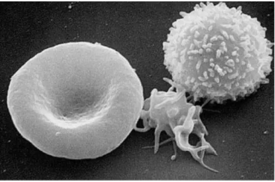
Blood is circulated around the body through blood vessels by the pumping action of the heart. Blood flow is a bodily flow that transport essential substances such as oxygen and nutrients to the cells and take away metabolic wastes from the same cells. In vertebrates, blood is composed by blood plasma, platelets, red blood cells and white blood cells. The main part of blood is plasma, which is a Newtonian fluid and constitutes around 55% of blood fluid (the large part of it is water). The rest 45% is red blood cells , while white blood cells and platelets only occupy less than 1% in blood. The white blood cells are the cells of the immune system that are involved in defending the body against both infectious disease and foreign materials; the main function of platelets is to stop bleeding. A scanning electron microscope image of a normal red blood cell, a platelet, and a white blood cell is shown in Figure 1.1.

Red blood cells (RBCs), also called erythrocytes, delivering oxygen (O2) to the

body tissues via the blood flow through the circulatory system. They take up oxygen in the lungs or gills and release it by diffusing thorough membrane of RBC into tis-sues while squeezing through the body’s vessels. RBCs are also able to transport 2% carbon dioxide (CO2) away from organisms while the major part of CO2 are

Figure 1.1: The cells in blood. From left to right: red blood cell, platelet and white blood cell.

by a cytoskeleton network embedding different kinds of proteins, as sketched in Fig-ure. 1.2. The proteins of the membrane skeleton are responsible for the deformability, flexibility and durability of the red blood cell. In general, a healthy RBC exhibits in biconcave shape (see Figure. 1.1) to accommodate maximum carry of oxygen; the shape of RBC is flexible, especially it can highly deformed while flowing thorough tiny capillaries with blood.

Figure 1.2: A cartoon showing major proteins on the membrane of RBC.

As mentioned in previous paragraph, the model of RBCs is quite complex due to variety features on its cell membrane. In order to grasp the fundamentals of blood flow and link them to the properties of RBCs, we consider a model system of vesicles. Vesicles are fluidic drops which is similar to the one surrounding living cells without cytoskeleton network structures (compare to RBCs). The most feature of vesicle is that it can be viewed as an approximation model of RBC. The membrane of vesicles has similar properties to the membrane of RBCs, resisting strongly surface dilatation

and exhibits a resistance against bending. Despite the simplicity structure of vesicle, many features observed by RBCs were also observed by vesicles. The mechanical details of vesicles will be introduced later in Chapter 2.

1.2

Existing works

For the past years, the vesicle problems have been extensively explored by the classic [24] and small deformation theories [40, 32, 12], flow experiments [26, 10], and com-puter simulations [25, 3, 45, 66, 67, 28, 4, 60, 68, 72]; just to name a few recent ones. Readers who are interested in more details on those relevant works can refer to the recent article [72].

The study of vesicle dynamics is a fluid-structure interaction problem. The nu-merical simulation of the problem consists of not only solving a two-phase flow but also requiring to enforce an inextensibility constraint along the surface which makes the problem challenging. Among the numerical methods for simulating vesicle prob-lems in literature, one can characterize those methods by how the membrane surface (or interface) is represented and what the fluid solver is used. Based on this charac-terization, several methods have been developed such as boundary integral method [25, 66, 67, 4, 68, 72], level set method [41, 60, 36, 43, 11], phase field method [9, 3, 43], particle collision method [45], immersed interface method [35, 65], and immersed boundary method [28, 37] et. al.

1.3

Immersed boundary method

The immersed boundary (IB) method proposed by Peskin [48] has been successfully applied to many fluid-structure interaction problems, see the review [50]. The IB formulation employs an Eulerian description for the fluid velocity and the pressure, and Lagrangian description for the configuration of the immersed elastic structure (immersed boundary or interface). The immersed structure exerts some force into the fluid that drives the fluid flow and at the same time the fluid flow carries the immersed structure to a new configuration. This interaction between the fluid and the immersed structure is linked through a force spreading and velocity interpolating operator by the usage of smoothed version of Dirac delta function [50]. This method is easy to implement and efficient simply because the immersed structure (no matter how complex) is regarded as a force generator to the fluid so the fluid variables can be solved in a fixed Eulerian domain without generating any structure-fitting grid. Therefore, many fast efficient fluid solvers can be applied through the framework of IB method. We will introduce the numerical part of IB method in detail in Chapter 3.

1.4

Contribution of the present work

In this dissertation, we focus on developing numerical method to mimic vesicle rhe-ology dynamics through IB method. For two-dimensional space, we propose a frac-tional step IB method and uncondifrac-tionally energy stable method, then we extend to three-dimensional axial symmetric coordinate by using a nearly inextensible approach. These works are based on our previous work [37, 22, 23]. The brief descriptions of numerical method are illustrated as below.

• Fractional step immersed boundary method. The governing equation is an incompressible Stokes equation with a suspension of inextensible interface (that is, the bending rigidity is neglected). We found that the spreading opera-tor of force generaopera-tor has skew-adjoint property to surface divergence operaopera-tor both in theoretical continuous and numerical discrete version. By taking advan-tage of this crucial property, the time-stepping numerical discretization involves solving a symmetric positive semi-definite matrix, and this linear system can be done efficiently by employing a preconditioned conjugate gradient method. We successfully reproduce vesicle-like dynamics such as tank-treading motion under shear flow. As a benchmark, we also measure the inclination angle and tank-treading frequency when reaching steady state. The numerical result shows a highly agreement with those in many other literatures.

• Unconditionally energy stable immersed boundary method. The fluid equation is governed by a Navier-Stokes equation with suspension of vesicle. Rather than enforcing purely inextensible constrain, we adopt a nearly inexten-sible approach to simulate vesicle dynamics. The fluid equations are discretized by projection method so the pressure is decoupled. Again by using skew-adjoint property, it leads to solve a symmetric positive sparse linear system respect to intermediate fluid variable, this can be done efficiently by aggregation-based multigrid. Meanwhile, we prove that the developed scheme shows an uncondi-tional stability in energy sense, which means the total energy of fluid system decreases during time integration. This is a significant step to release restric-tion of numerical time step due to applying the penalized method. Again we successfully simulated vesicle dynamics, such as a free relaxation to equilibrium state, tank-treading motion under shear flow, the numerical cost is substantial saved by this scheme.

• Simulating three-dimensional axisymmetric vesicles. We extend previ-ous work to three-dimensional space to link the real world. An axisymmetric vesicle is suspended in incompressible Navier-Stokes flow in three-dimensional capillary. Again the nearly inextensible approximation in axisymmetric version is applied. We have shown that the modified interfacial force due to nearly inex-tensible approaching has exactly the same form to the original one. Besides, we

adopt a high accuracy spectral method to evaluate interfacial quantities such as mean curvature, Gaussian curvature and surface Laplace of mean curvature. The fluid variables are solved numerically by traditional projection method in which fast Poisson solver can be applied to obtain fluid velocity filed and pres-sure increment. We investigated behaviors of axisymmetric vesicle in situation of freely suspended, under influence of gravity field and passing through capil-lary in Poiseuille flow. The numerical result shows a good agreement with what observed in experiment, and this is an evidence showing the reliability of our proposed scheme.

Chapter 2

Mathematical model of vesicle

hydrodynamics

The first model used for vesicles can be tracked back to Helfrich (1973) [18], who inves-tigated the rheology dynamics of vesicle through a elasticity theory. In this chapter, we introduce more details about vesicle, such as vesicle mechanism, the vesicle sur-face energy and the the boundary forces on vesicle membrane. The mathematical formulation of hydrodynamical system for suspended vesicle is given.

2.1

Vesicle mechanics

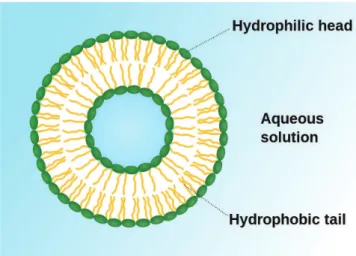
A vesicle can be visualized as a liquid droplet within another liquid enclosed by a lipid membrane with the size about 100 nm to 10 µm. Such lipid membrane consists of tightly packed lipid molecules with hydrophilic heads facing the exterior and inte-rior fluids and with hydrophobic tails hiding in the middle and thus forms a bilayer phospholipid with thickness about 6 nm (see Figure 2.1).

Vesicle is widely used for mimicking model of biological cells and also gives many features observed by living cells. The shape of vesicle is deformable, in equilibrium state, the vesicle usual appears in shape of biconcave disk because of minimized surface energy (see Figure 2.2). Topological changes (fusion, division, etc.) of vesicle are possible but rarely happened in real world. In principle, the vesicle membrane mainly undergoes two basic deformation factors, which are inextensibility and bending

effect.

At usual room temperature, since the phospholipidic molecules do not bind with each other, the membrane is thus regard as a liquid phase. In this scenario, phos-pholipids stay very close and tend to approximate a constant density, it would lead to local conservation of vesicle surface. Therefore, the membrane is considered as an inextensible surface. Moreover, because the permeability of vesicle membrane is very small and fluid inside vesicle is Newtonian incompressible fluid, this contributes to

Figure 2.1: A cartoon showing a vesicle and its molecular structure on membrane. Picture is taken from the web site of Wikipedia.

Figure 2.2: Biconcave equilibrium state of vesicles.

total volume of vesicle is conserved as well. The phospholipid membrane is known to exhibit a resistance against bending, we have to take bending effect into account in our mathematical formulation.

In consequence, we list three features of vesicle as below.

• The total surface area of vesicle is conserved because of the inextensibility. This is the intrinsic feature of vesicle which is regarded as a simplified model of red blood cell. The mathematical formulation of inextensibility will be explained later in Section 2.3.

• The total volume of vesicle remains a constant since it contains incompressible Newtonian fluid. The mathematical statement is shown in Section 2.4.

• The bending effect should be considered in modeling vesicle dynamics. The explicit form of bending force is given in Section 2.2.

When it comes to vesicle dynamics, we must mention a dimensionless characteristic variable, the reduced volume, which measures the deflation of the vesicle, plays a significant role in the vesicle dynamics. It is defined as

ν3D ₌ V0

4

3π(S0/4π)3/2

,

where V0 and S0 represent the volume and the surface area of vesicle, respectively.

This dimensionless number is nothing but the volume ratio of the vesicle to a sphere with the same surface area, and thus is equal to 1 for a sphere. In two dimensions a parameter equivalent to reduced volume is defined by reduced area, which is defined by

ν2D ₌ A0

π(L0/2π)2

,

where A0 and L0 denote for the area and the arc-length of vesicle respectively. Again

this definition follows the ratio of the vesicle to a circle with the same arc-length. In the rest of dissertation, we would use the notation ν to denote reduced volume (3D) or reduced area (2D) for convenience.

2.2

Interfacial forces on vesicle

A vesicle membrane is known to be inextensible and exhibits a resistance against bending. Thus, the membrane energy can be modeled by two parts; namely, the elastic tension energy Eσ to enforce the inextensibility constraint [71], and the Helfrich type

energy Eb [18] to resist the bending of the membrane. A way to derive the interfacial

forces on vesicle is from the energy point of view, a variational method. Assume E[X] is an energy functional corresponding to vesicle configuration X (or interface), we can obtain the interfacial force F by taking variational derivative as

F = −δE[X]

δX ,

where δX is a perturbation on interface. In next subsection, the mathematical defi-nition of two energies Eσ and Eb are given in both two and three-dimensional space,

and the corresponding interfacial force are obtained.

2.2.1

In two dimensions

Let us define the vesicle by Γ(t), and its configuration is presented by X = X(s, t) = (X(s, t), Y (s, t)), 0 ≤ s ≤ Lb, where s is a Lagrangian parameter along interface. The

outward of interface) are denoted by τ and n respectively, and these two vectors can be obtained by τ = (τ1, τ2) = Xs |Xs| and n = (n1, n2) = (τ2, −τ1).

The total vesicle energy E(t) which consists of elastic and bending energy is defined by E(t) = Eσ(t) + Eb(t) = Z Γ σ ds + cb 2 Z Γ κ2 ds,

where σ is the surface tension, κ is the curvature and cb is the strength of

bend-ing rigidity. Let us get start the process of variational derivative. Denote eX(s) = ( eX(s), eY (s)) as a perturbation of the interface X (omit time variable t) and ε as a

small number. Then the perturbed elastic energy becomes

Eσ(X + ε eX) =

Z _Lb

0

σ|Xs+ ε eXs| ds.

Taking the derivative of above energy with respect to ε, we obtain

dEσ dε (X + ε eX) = Z _Lb 0 σ(Xqs+ ε eXs) eXs+ (Ys+ ε eYs) eYs (Xs+ ε eXs)2+ (Ys+ ε eYs)2 ds. Then we evaluate the above equation at ε = 0 to obtain

dEσ dε (X + ε eX) ¯ ¯ ¯ ¯ ¯ ε=0 = Z _Lb 0 σ Xs |Xs| · eXs ds = Z _Lb 0 στ · eXs ds = στ · eX ¯ ¯ ¯ ¯ ¯ Lb 0 − Z _Lb 0 ∂ ∂s(στ ) · eX ds (integration by part) = − Z _Lb 0 ∂ ∂s(στ ) · eX ds.

This leads to the corresponding elastic tension force Fσ =

∂

∂s(στ ). (2.1)

Especially notice that, if tension σ is a constant (for the case of clean droplet), then the elastic tension force would act only along normal direction of interface. On the other hand, for obtaining the bending force we perturb the bending energy by

Eb(X + ε eX) = cb 2 Z _Lb 0 ¯ ¯ ¯ ¯∂ 2_{X + ε eX} ∂s2 ¯ ¯ ¯ ¯ 2 ds.

Taking derivative with respect to ε obtains dEb dε (X + ε eX) ¯ ¯ ¯ ¯ ¯ ε=0 = cb Z _Lb 0 ∂X + ε eX ∂s2 ∂2_Xe ∂s2 + ∂Y + ε eY ∂s2 ∂2_Ye ∂s2 ds = cb Z _Lb 0 ∂2_X ∂s2 · ∂2_Xe ∂s2 ds = − Z _Lb 0 −cb∂ 4_X

∂s4 · eX ds (integration by part twise)

Therefore we obtain the explicit form of bending force as Fb = −cb

∂4_X

∂s4 . (2.2)

Notice that there is another remarkable version of bending force as Fb = cb µ ∂2_κ ∂s2 + κ3 2 ¶ n. (2.3)

One can see the derivation in detail in [27]. Throughout this dissertation, we select the two-dimensional bending force Fb in Eq. (2.2).

2.2.2

In three dimensions

In three-dimensional case, the vesicle surface is presented by parametric form as X(α, β, t) = (X(α, β, t), Y (α, β, t), Z(α, β, t)), 0 ≤ α ≤ Lα and 0 ≤ β ≤ Lβ, where α

and β are two Lagrangian parameters. The total energy of vesicle is defined by

E(t) = Eσ(t) + Eb(t) = Z Γ σ dS + cb 2 Z Γ H2 dS,

where H is the surface mean curvature and dS is the local surface element. By taking variational derivative to the surface energy, one can derive the vesicle boundary force consisting of the elastic force Fσ and the bending force Fb as

Fσ = ∇sσ − 2Hσn and Fb = cb

¡

∆sH + 2H(H2− K)

¢

n, (2.4) where K is the Gaussian curvature respectively, ∇s is the surface gradient operator,

and ∆s is the surface Laplacian operator. The detailed derivation can be found in

[69]. The computation of these geometrical quantities and operators can be obtained by geometrical fundamental form, ant they are given in detail in Appendix A.

Remark: Notice that there are terms of derivative of function along interface hap-pened in the interfacial force term, especially fourth derivative of interfacial position is involved when evaluating bending force. These terms shall be treated very carefully in numerical simulation due to there might be a contributed interfacial stiffness.

2.3

Inextensible formulation

As mentioned previously, the vesicle exhibits inextensible property, which means the local surface element conserves as a quantity, and obviously this leads to conservation of global surface area of vesicle. The mathematical description of inextensibility in two and three-dimensional spaces are shown in the following.

2.3.1

In two dimensions

In two-dimensional space, the vesicle is represented by closed curve and its local arc-length is conserved. It is straightforward to write changing rate of local arc-arc-length by ∂ ∂t(|Xs|) = ∂ ∂t ³p X2 s + Ys2 ´ = XsXst+ YsYst |Xs| = ∂U ∂s · τ = (∇s· U) |Xs| , (2.5) where U = ∂X

∂t denotes for velocity defined on the vesicle (interface). From Eq. (2.5),

since local arc-length does not change with time varying, i.e. ∂

∂t(|Xs|) = 0, we can

deduce that surface divergence of velocity must be zero, that is

∇s· U = 0. (2.6)

2.3.2

In three dimensions

In three-dimensional case, we start by using the fact

|Xα× Xβ| n = Xα× Xβ.

Then taking time derivative to the above equation obtains

∂ ∂t(|Xα× Xβ|) n + |Xα× Xβ| ∂n ∂t = ∂ ∂t(Xα× Xβ) .

By taking inner product of n on the both side of above equation, we have

∂ ∂t(|Xα× Xβ|) = ∂ ∂t(Xα× Xβ) · n = n · (Uα× Xβ) + n · (Xα× Uβ) = Uα· (Xβ × n) + Uβ· (n × Xα) = Uα W (Xβ× (Xα× Xβ)) + Uβ W ((Xα× Xβ) × Xβ) = Uα W (GXα− F Xβ) + Uβ W (EXβ − F Xα) = GUα− F Uβ W · Xα+ EUβ − F Uα W · Xβ = (∇s· U) |Xα× Xβ| .

Notice that we use the notation of first fundamental form (refer to Appendix A). One can see that, from the above equation, inextensible property again leads zero surface divergence of velocity field as

∇s· U = 0. (2.7)

In summary, inextensible property is equivalent zero surface divergence of velocity field as in Eqs. (2.6) and (2.7), and this is regarded as an additional constraint. In fact, tension plays a role as Lagrangian’s multiplier to enforce inextensibility, we will explain it in detail in later section.

2.4

Hydrodynamical equations

In previous section, the membrane driven force of vesicle is obtained by minimizing total vesicle energy. The next step is to couple the motion of equation for fluid to the membrane force. The framework of fluid vesicle mechanism system will be clearly stated in this section.

2.4.1

Incompressible Navier-Stokes equations

Firstly, we begin by explaining mathematical formulation of fluid incompressibility. Consider a specific system of fluid with control volume V (shape can change with time), but the total mass does not change. Denote density by ρ and velocity field by u, under Lagrangian framework, by tracking total mass of this control volume, the mass conservation law is stated as

D Dt Z V (t) ρ dV = 0, (2.8) where D

Dt = ∂t∂ +u·∇ denotes for material derivative. By Reynolds transport theorem,

the above equation can be written by Z

V ∂ρ

∂t + ∇ · (ρu) dV = 0. (2.9)

Since control volume is arbitrary chosen, the integrand in Eq. (2.9) is always zero, i.e.,

∂ρ

∂t + ∇ · (ρu) = 0. (2.10)

Eq. (2.10) is called continuity equation and can be alternatively written in the form of

Dρ

For incompressible fluid, shape of control volume can change but mass and volume remain, that is, the density of fluid element remains constant. Under this assumption, we can deduce Dρ_Dt = 0, thus mass conservation law of Eq. (2.11) is reduced by

∇ · u = 0. (2.12)

The Navier-Stokes equation is govern by conservation law of momentum. In clas-sical mechanics, momentum is the product of the mass and velocity of an object. The conservation of momentum describes the total amount of momentum within a control volume keeps as a constant. That is to say, momentum is neither created nor destroyed, but it can be changed by external forces. Actually, the conservation of momentum is an application of Newton’s second law of motion, which states the rate change of momentum of a fluid mass is equal to net external forces acting one the mass. Such external forces are consisted of two classes. One is the body force (body force per unit mass), gravitational force or electromagnetic force for instance; the other one is surface force (surface force per unit area), such as pressure forces or viscous stress.

With basic physical property of fluid mechanics, now we begin to introduce math-ematical formulation of Navier-Stokes equation. We assume the fluid is Newtonian, based on constitutive law, the expression for stress tensor is

σij = −pδij + µ µ ∂ui ∂xj +∂uj ∂xi ¶ , (2.13)

where δij presents Kronecker delta function (δij = 1 if i = j; δij = 0 if i 6= j), p

is the pressure and µ is the viscosity. Throughout this dissertation, the density and viscosity are both assumed to be uniform constant. Coupling the fluid incompress-ibility constrain Eq. (2.12), the mathematical equations of motion consist of a viscous incompressible fluid in a domain Ω can be written as follows.

ρ µ ∂u ∂t + (u · ∇) u ¶ = ∇ · σij = −∇p + µ∆u in Ω, ∇ · u = 0 in Ω.

Notice that there is no equation describing evolution of pressure p. In fact, pressure p plays a role as Lagrange’s multiplier to enforce the fluid incompressibility constraint. On the other hand, for well-poseness of Navier-Stokes equation, the velocity field is equipped with boundary condition, and we name several types of boundary condition as follows.

• No-slip boundary condition: There is no fluid which penetrates the boundary, the fluid is at rest status on boundary, that is

• Inflow boundary condition: The velocity field is given specifically on the bound-ary, that is

u|∂Ω= ub.

• Outflow boundary condition: Neither velocity component changes in normal direction to the boundary, that is

∂u

∂n = 0.

2.4.2

Coupling the fluid equations to vesicle forces

In this section, the governing equation of fluid motion and force acting on vesicle membrane are combined by Immersed boundary formulation. In immersed boundary framework, the fluid variables (velocity field, pressure, etc.) are defined in Eulerian coordinate and interfacial variables (membrane position, membrane force, etc.) are defined in Lagrangian coordinate. These two types of variable are linked by inter-action equations in which the Dirac delta function plays a prominent role. Now we come to state the whole fluid system of vesicle dynamics through immersed boundary method in two-dimensional space. The mathematical equations of motion consist of a viscous incompressible fluid in a domain Ω containing an immersed, inextensible, massless vesicle boundary (or interface) Γ(t) which can be written in an immersed boundary formulation as ρ µ ∂u ∂t + (u · ∇)u ¶ = −∇p + µ∆u + Z Γ F(s, t)δ(x − X(s, t)) ds in Ω, (2.14) ∇ · u = 0 in Ω, (2.15) ∇s· U = 0 on Γ, (2.16) ∂X ∂t (s, t) = U(s, t) = Z Ω u(x, t)δ(x − X(s, t)) dx on Γ. (2.17) The interfacial force F consists of tension and bending force as

F = Fσ+ Fb = ∂

∂s(στ ) − cb ∂4_X

∂s4 . (2.18)

Eqs. (2.14)-(2.15) are the incompressible Navier-Stokes equations with a singular force term F arising from the vesicle membrane force. Eq. (2.16) represents the inextensibility constraint of the vesicle surface which is equivalent to the zero surface divergence of the velocity along the interface. Eq. (2.17) simply explains that the interface moves along with the local fluid velocity (the interfacial velocity). Here, the

interfacial velocity U is the interpolation of the fluid velocity at the interface defined as in traditional IB formulation. The interaction between the fluid and the interface is linked by the two-dimensional Dirac delta function δ(x) = δ(x)δ(y). One can easily extend to fully three-dimensional Navier-Stokes equation by taking three-dimensional vesicle membrane force mentioned previously.

It is worthy to mention that, in fact, the tension σ acts like a Lagrange’s multiplier function to enforce the local inextensibility constraint along the surface which is exactly the same role played by the pressure to enforce the fluid incompressibility in Navier-Stokes equations. Therefore, the development of an efficient and accurate algorithm for vesicle dynamics remains quite challenging; not to mention the vesicle surface moves along with the surrounding fluid as well.

Chapter 3

Immersed boundary method

The immersed boundary (IB) method was firstly proposed by Peskin [48] to simulate blood heart value problems. The IB method has found a wide variety of applications in biological mechanics and has been successfully applied to study fluid-structure interaction problems. The main idea of IB method is to treat Lagrangian material as a part of fluid in which arises additional interfacial forces. The fluid variables are solved in regular Cartesian domain (uniform rectangular lattice) without any modification of fluid equation; the interface is tracked by a set of discrete Lagrangian markers which can freely move in Eulerian domain and the shape of interface can has complex geometry. The interfacial forces can be computed through spatial position of Lagrangian markers and only has effect in its vicinity fluid, i.e. these forces are spread into its surrounding fluid lattices. With presence of these forces, the new fluid velocity can be obtained. The interface position is then advanced by this new fluid velocity through an interpolation.

3.1

Connection between fluids and interfaces

In this section, we introduce the linkage between fluid equation and Lagrangian in-terface. By taking advantage of Dirac delta function, a value of function can be obtained through product with a shifted delta source function, and then integrate over the whole space (thus the shifted delta function is regarded as a kernel of in-tegral). We clarify this definition by writing the spreading forces on Cartesian grid by

f(x, t) = Z

Γ

F(s, t) δ(x − X(s, t)) ds, (3.1) and the interpolation of fluid velocity field by

u(X(s, t), t) = U(s, t) = Z

Ω

Notice that Eqs. (3.1) and (3.2) represent for a line integral along the interface and an area integral over whole fluid domain respectively (in three-dimensional case, they are surface and volume integral). It is interesting to see that the total amount of singular force in Eq. (3.1), which is an integral of f(x, t) over whole domain, is equal to the total force on the immersed interface. This means although the interfacial forces (force per length) are converted to body force (force per area), the total amount of applied body force still preserves to act on the fluids. The important feature of IB method is Eq. (3.1) converts Lagrangian to Eulerian coordinate while Eq. (3.2) does in opposite direction.

3.2

Discrete delta function

As mentioned in previous section, the major novelty of IB method is introducing a delta function, which plays an important role converting coordinate between Eulerian and Lagrangian manner. Since delta function is in a view point of distribution under generalized function theorem, in the aspect of numerics, the discrete version of delta function shall be acquired.

The discrete version of delta function δh(x) should be smooth enough to guarantee

the smoothness of distribution of Eqs. (3.1) and (3.2), and has compact support in a narrow region to ensure the numerical efficiency when computing spreading and interpolation. A two-dimensional delta function is required to be the form of

δh(x) = 1 h2φ ³x h ´ φ³ y h ´ ,

where x = (x, y), φ(r) is a real function, and δh → δ as h → 0. We say φ(r) has moment condition of order q if

X i (α − i)r_{φ(α − i) =} ½ 1, r = 0 0, 1 ≤ r ≤ q − 1 (3.3) for all values of α. When r = 0, ensures total mass of the discrete delta function is identically one. The moment condition (3.3) represents for the numerical accuracy of interpolation. For instance of one-dimensional case, suppose φ has moment condition

q, let f be a real smooth function and α be an arbitrary real number, we have

f (α) − hX

i

f (xi)δh(xi− α) = O(hq),

where xi = ih. The above equation can be done directly by using Taylor expansion

on f (xi) at the point x = α. Now we list several regular discrete functions which are

popular and widely used in lot of literatures. They are the 2-point hat function φ1

[29], the 4-point cosine function φ2 [48], the 3-point discrete function φ3 [54], and the

4-point piecewise function φ4 [50] as follows (with moment condition of order 2,1,2

• A 2-point hat function φ1:

φ1(r) =

½

1 − |r|, |r| ≤ 1, 0, 1 ≤ |r|.

• A 4-point cosine function φ2:

φ2(r) = ½ ₁ 4 ¡ 1 + cos(πr 2 ) ¢ , |r| ≤ 2, 0, 2 ≤ |r|. • A 3-point function φ3: φ3(r) =      1 3(1 + √ −3r2_{+ 1), |r| ≤ 0.5,} 1 6 ³ 5 − 3|r| −p−3(1 − |r|)2_{+ 1} ´ , 0.5 ≤ |r| ≤ 1, 0, 1.5 ≤ |r|. • A 4-point function φ4: φ4(r) =        1 8 ³ 3 − 2|r| +p1 + 4|r| − 4r2´_{, |r| ≤ 1,} 1 8 ³ 5 − 2|r| −p−7 + 12|r| − 4r2 ´ , 1 ≤ |r| ≤ 2, 0, 2 ≤ |r|.

However, it has been found that with these regular discrete functions, a non-physical oscillations might happened in numerical simulation which is mainly due to the deriva-tive of regular functions do not satisfy certain moment condition. In [70], the authors developed an simple smoothing technique for discrete delta function φ∗_{(r) by}

extend-ing a half mesh wider support as

φ∗_{(r) =}

Z _r+0.5

r−0.5

φ(r0_{) dr}0_{. (3.4)}

In terms of the definition (3.4), the smoothed functions φ∗

1, φ∗2, φ∗3 and φ∗4

correspond-ing to φ1, φ2, φ3 and φ4 can be formulated as follows.

• A smoothed 2-point hat function φ∗

1: φ∗ 1(r) =    3 4 − r2, |r| ≤ 0.5, 9 8 − 32|r| + r 2 2, 0.5 ≤ |r| ≤ 1.5, 0, 1.5 ≤ |r|.

• A smoothed 4-point cosine function φ∗ 2: φ∗ 2(r) =    1 4π £ π + 2 sin¡π 4(2r + 1) ¢ − 2 sin¡π 4(2r − 1) ¢¤ , |r| ≤ 1.5, − 1 8π £ −5π + 2π|r| + 4 sin¡π 4(2|r| − 1) ¢¤ , 1.5 ≤ |r| ≤ 1.5, 0, 2.5 ≤ |r|.

• A smoothed 3-point function φ∗

3: φ∗ 3(r) =                17 48 + √ 3π 108 + |r| 4 − r 2 4 + 1−2|r| 16 p −12r2_{+ 12|r| + 1} −√3 12 sin−1 ³√ 3 2 (2|r| − 1) ´ , |r| ≤ 1, 55 48 − √ 3π 108 − 13|r| 12 + r 2 4 + 2|r|−3 48 p −12r2_{+ 36|r| − 23} +√3 36 sin−1 ³√ 3 2 (2|r| − 3) ´ , 1 ≤ |r| ≤ 2, 0, 2 ≤ |r|.

• A smoothed 4-point function φ∗

4: φ∗ 4(r) =                  3 8 + π 32− r2 4, |r| < 0.5, 1 4 + 1−|r| 8 p −2 + 8|r| − 4r2₋1 8sin −1¡√_{2(|r| − 1)}¢_{, 0.5 ≤ |r| ≤ 1.5,} 17 16 − π 64 − 3|r| 4 + r2 8 + |r|−2 16 p −14 + 16|r| − 4r2 +1 16sin−1 ¡√ 2(|r| − 2)¢, 1.5 ≤ |r| ≤ 2.5, 0, 2.5 ≤ |r|.

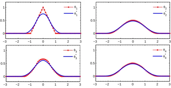
A comparative plot between regular function φ and corresponding smoothed func-tion φ∗ _{are depicted in Figure. 3.1. To summarize, we list the advantages of smoothed}

function below.

• Through Eq. (3.4), the smoothed function has a half mesh wider support and gains one higher derivative than regular one

• The moment conditions of smoothed function are preserved from original regular function except φ∗

2 gains moment condition of order 2.

• The derivative of smoothed functions φ0_{(r) have one order higher moment}

con-dition than φ(r).

One can refer the details of proof for last two points in [70]. In our numerical exper-iments, the smoothed delta function indeed benefits not only improving the stability of whole numerical scheme, but also removing nonphysical interfacial oscillation. We take φ∗

4 as a standard to construct discrete delta function throughout all numerical

−3 −2 −1 0 1 2 3 0 0.5 1 r −3 −2 −1 0 1 2 3 0 0.5 1 r −3 −2 −1 0 1 2 3 0 0.5 1 r −3 −2 −1 0 1 2 3 0 0.5 1 r φ₁ φ₁* φ₂ φ₂* φ₃ φ₃* φ₄ φ₄*

Figure 3.1: The figure of discrete function φi (i = 1, 2, 3, 4) and correspond smoothed

functions φ∗

i (i = 1, 2, 3, 4).

3.3

Numerical setup

In this section, we introduce a numerical setup for spatial discretization based on standard finite difference method in detail. Firstly, a famous and traditional stag-gered grid is applied for discretization of fluid equations. Under layout of stagstag-gered grid, fluid equations can be solved accurately by some existing fluid solver, such as projection method. Secondly, the usage of boundary conditions and approximation of values at ghost point will be carried out. Lastly, the numerical setting of interfacial values are presented.

3.3.1

Staggered grid

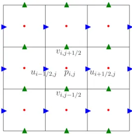
The staggered marker-and-cell (MAC) grid was proposed by Harlow and Welsh [17] to simulate viscous impressible flow with free surface. The rectangular computational domain Ω is set by Ω = [a, b] × [c, d], speaking in detail, the pressure is defined on the grid points labeled as x = (xi, yj) = (a + (i − 1/2)4x, c + (j − 1/2)4y), i = 1, 2, · · · , m and j = 1, 2, · · · , n, while the velocity components u and v are

defined at (xi, yj−1/2) = (a + (i − 1)4x, c + (j − 1/2)4y) and (xi−1/2, yj) = (a + (i −

1/2)4x, c + (j − 1)4y), respectively. Here, we assume that a uniform mesh width

h = 4x = 4y is used, although that is not necessary. One can see the sketch of

staggered grid from Figure 3.2.

Let us demonstrate a standard second-order finite difference method based on stag-gered grid for fluid equation. In two-dimensional space, the incompressible

Navier-r r r r r r r r r I I I I I I I I I I I I N N N N N N N N N N N N pi,j ui−1/2,j ui+1/2,j vi,j−1/2 vi,j+1/2

Figure 3.2: The layout of staggered grid in two-dimensional rectangular domain. The red dots indicate location of pressure p, while the green and blue triangles represent for velocity component u and v respectively.

Stokes equation is expressed explicitly by

ρ µ ∂u ∂t + u ∂u ∂x + v ∂u ∂y ¶ = −∂p ∂x + µ µ ∂2_u ∂x2 + ∂2_u ∂y2 ¶ + f, (3.5) ρ µ ∂v ∂t + u ∂v ∂x + v ∂v ∂y ¶ = −∂p ∂y + µ µ ∂2_v ∂x2 + ∂2_v ∂y2 ¶ + g, (3.6) ∂u ∂x + ∂v ∂y = 0, (3.7)

where f and g represent external forces. Let start with discretization of fluid incom-pressibility in Eq. (3.7), a second-order accurate finite difference based on Figure. 3.2 gives

ui+1/2,j− ui−1/2,j

h +

vi,j+1/2− vi,j−1/2

h = 0. (3.8)

derivatives with respect to space for (i, j)-cell are computed by µ u∂u ∂x ¶ i+1/2,j = ui+1/2,j ui+3/2,j − ui−1/2,j 2h , µ v∂u ∂y ¶ i+1/2,j = vi+1/2,j ui+1/2,j+1− ui+1/2,j−1 2h , µ ∂p ∂x ¶ i+1/2,j = pi+1,j− pi,j h , µ ∂2_u ∂x2 ¶ i+1/2,j

= ui−1/2,j− 2ui+1/2,j+ ui+3/2,j

h2 , µ ∂2_u ∂y2 ¶ i+1/2,j

= ui+1/2,j−1− 2ui+1/2,j + ui+1/2,j+1

h2 , µ u∂v ∂x ¶ i,j+1/2 = ui,j+1/2 vi+1/2,j+1− ui+1/2,j−1 2h , µ v∂v ∂y ¶ i,j+1/2 = vi,j+1/2 vi,j+3/2− vi,j−1/2 2h , µ ∂p ∂y ¶ i,j+1/2 = pi,j+1− pi,j h , µ ∂2_v ∂x2 ¶ i,j+1/2

= vi−1,j+1/2− 2vi,j+1/2+ vi+1,j+1/2

h2 , µ ∂2_v ∂y2 ¶ i,j+1/2

= vi,j−1/2− 2vi,j+1/2+ vi,j+3/2

h2 .

Notice that the terms ui,j+1/2and vi+1/2,j do not show up in staggered grid formation,

and these two terms can be evaluated by a second-order linear interpolation as

ui,1+1/2 =

1 4

¡

ui−1/2,j+ ui+1/2,j+ ui−1/2,j+1+ ui+1/2,j+1

¢ , vi+1/2,j = 1 4 ¡

vi,j−1/2+ vi+1,j−1/2+ vi,j+1/2+ vi+1,j+1/2

¢

.

In further chapters, we will use the notations ∇h, ∇h· and ∆hto denote for numerical

gradient, divergence and Laplace mentioned above.

3.3.2

Ghost values from boundary conditions

In this section, we demonstrate the evaluation of approximation for ghost values due to they are used in fluid solver. In staggered grid formation, the pressure is define on a cell center, while velocity component u and v are on cell face.

In our numerical simulation, we always assume that u is given on x = a and

x = b, and v is also known on y = c and y = d. That is, Dirichlet boundary

conditions (either no-slip or inflow) are assigned to u(a, y), u(b, y), v(x, c) and v(x, d). For the rest boundary conditions ,u(x, c), u(x, d), v(a, y) and v(b, y), can be set as either Dirichlet or Neumann boundary type. Under this assumption, the boundary values of u1/2,j and um+1/2,j can be obtained exactly corresponding to its boundary

conditions u(a, y) and u(b, y), as well as boundary values of vi,1/2 and vi,n+1/2 to v(x, c) and v(x, d). Therefore, the ghost points are ui+1/2,0, ui+1/2,m+1, v0,j+1/2 and

vm+1,j+1/2. We separate two types of boundary condition to approximate those ghost

values bellow.

• Dirichlet boundary condition: The value of ghost point is evaluated by a second-order extrapolation as follows.

ui+1/2,0 = 2u(xi+1/2, c) − ui+1/2,1, ui+1/2,n+1 = 2u(xi+1/2, d) − ui+1/2,n,

v0,j+1/2 = 2v(a, yj+1/2) − v1,j+1/2,

vm+1,j+1/2 = 2v(b, yj+1/2) − vm,j+1/2.

• Neumann boundary condition: Suppose the value of ∂u

∂y(x, c) is given, then

the ghost value ui+1/2,0 can be obtained by a central difference with local

trun-cation error O(h2_{) by}

ui+1/2,1− ui+1/2,0

h =

∂u

∂y(xi+1/2, c).

Rearranging the above equation gives

ui+1/2,0 = h ∂u

∂y(xi+1/2, c) − ui+1/2,1.

The other ghost values are computed in the similar way as

ui+1/2,n+1 = h

∂u

∂y(xi+1/2, d) + ui+1/2,n, v0,j+1/2 = h ∂v ∂x(a, yj+1/2) − v1,j+1/2, vm+1,j+1/2 = h ∂v ∂x(b, yj+1/2) + vm,j+1/2.

3.3.3

Lagrangian manners

For the immersed interface X, we use a collection of discrete points sk = k∆s, k =

0, 1, · · · , M , with the interface mesh width ∆s so the Lagrangian markers of the interface are represented by Xk = X(sk). Other interfacial quantities, such as force

density F and velocity U are defined on position Xk so the notations Fk = F(sk)

and Uk = U(sk) are used. One can see the illustration of IB framework of regular

uniform grid and set of discrete Lagrangian markers in Figure 3.3.

Figure 3.3: The basic framework of IB method, spreading discrete Lagrangian markers in a computational domain with uniform mesh.

Especially pay attention that we often have to compute derivatives of interfacial quantities. For instance, the vesicle membrane forces which consist of tension and bending force involve evaluating derivatives of position Xk. Therefore calculation of

derivative along the interface plays an important role to the dynamics of the interface. Here we provide two ways to compute derivative of a function along interface. Without loss of generality, for any function defined on the interface ψ(s), we approximate the partial derivative ∂ψ_∂s by

• Finite difference method: The value of ∂ψ_∂s can be approached by standard second-order central difference scheme as

Dfψ(s) = ψ(s + ∆s/2) − ψ(s − ∆s/2)

∆s .

• Spectral method: Since ψ is assumed to be periodic along interface, we can adopt the spectral Fourier discretization to achieve higher-order of accuracy. The interface is represented by the discrete Fourier series expansion as

ψ(s) =

M/2−1_X k=−M/2

c

where cψk is the corresponding Fourier coefficients for ψ(s). This Fourier

coef-ficients can be performed very efficiently by using the Fast Fourier Transform (FFT). Then the Fourier coefficients of P -th derivative of ψ(s) can be obtained by taking an inverse FFT to (ik)Pc_ψ

Chapter 4

Fractional step immersed

boundary method

In this chapter, we develop a fractional step method based on IB formulation for Stokes flow with an inextensible interface (vesicle without bending stiffness). Solving the fluid variables such as the velocity and pressure, the present problem involves finding extra unknown elastic tension such that the surface divergence of the velocity is zero along the interface. Once the velocity is found, the interface is moving accord-ing to the local fluid velocity. Since the fluid is incompressible and the interface is inextensible, both the area enclosed by the interface and the total length of the in-terface should be conserved. Notice that, the dynamics of vesicles are determined by their boundary rigidity, inextensibility, and the hydrodynamical forces. Our present model for inextensible interface can be regarded as a simplified vesicle model without bending effect.

The rest of the chapter are organized as follows. In the next section, we describe our governing equations for the Stokes flow with an inextensible interface based on IB formulation. We also show the skew-adjoint property between the spreading oper-ator acting on the tension and the surface divergence of the velocity. In Section 4.2, the symmetry of the resultant matrix equation is provided first, and then a numerical algorithm based on the fractional step method is developed. Finally, the numerical re-sults including the convergence tests and the tank-treading motion for an inextensible interface under a simple shear flow are shown in detail in Section 4.4.

4.1

Governing equations

We begin by stating the mathematical formulation of the Stokes flow with an inex-tensible interface. Consider there is a moving, immersed, inexinex-tensible interface Γ(t) in the fixed fluid domain Ω. We assume that the fluids inside and outside of the interface are the same so the governing equations in IB formulation can be written