禪坐腦電波之時變頻譜的空間特性研究(II)

行政院國家科學委員會專題研究計畫 成果報告

禪坐腦電波之時變頻譜的空間特性研究(II)

研究成果報告(精簡版)

計 畫 類 別 ： 個別型 計 畫 編 號 ： NSC 97-2221-E-009-093- 執 行 期 間 ： 97 年 08 月 01 日至 98 年 07 月 31 日 執 行 單 位 ： 國立交通大學電機與控制工程學系（所） 計 畫 主 持 人 ： 羅佩禎 計畫參與人員： 碩士班研究生-兼任助理人員：楊淮璋 碩士班研究生-兼任助理人員：張家鈞 碩士班研究生-兼任助理人員：黃順敏 博士班研究生-兼任助理人員：黃瑄詠 博士班研究生-兼任助理人員：吳適達 博士班研究生-兼任助理人員：張致豪 其他-兼任助理人員：朱意屏 其他-兼任助理人員：許瑋婷 報 告 附 件 ： 出席國際會議研究心得報告及發表論文 處 理 方 式 ： 本計畫可公開查詢

中 華 民 國 98 年 12 月 23 日

行政院國家科學委員會補助專題研究計畫成果報告

禪坐腦電波之時變頻譜的空間特性研究(II)

Time-varying Spatio-spectral Characteristics of Meditation EEG

計畫類別：■個別型計畫 □整合型計畫

計畫編號：NSC 97-2221-E-009-093

執行期間：97 年 08 月 01 日 至 98 年 07 月 31 日

計畫主持人：羅佩禎

共同主持人：

成果報告類型（依經費核定清單規定繳交）：█精簡報告 □完整報告

本成果報告包括以下應繳交之附件：

□赴國外出差或研習心得報告一份

■出席國際學術會議心得報告及發表之論文各一份

□國際合作研究計畫國外研究報告書一份

處理方式： 除產學合作研究計畫、提昇產業技術及人才培育研究計畫、列

管計畫及下列情形者外，得立即公開查詢

□涉及專利或其他智慧財產權，□一年□二年後可公開查詢

執行單位：國立交通大學 電機與控制工程學系

中 華 民 國 九十八 年 九 月 二十七 日

行政院國家科學委員會專題研究計畫成果報告

禪坐腦電波之時變頻譜的空間特性研究(II)

Time-varying Spatio-spectral Characteristics of Meditation EEG

計畫編號： NSC 97-2221-E-009-093

執行期限： 97年08月01日至98年7月31日

主 持 人： 羅佩禎，國立交通大學 電機工程學系

中文摘要

過去十年來，主持人將醫學工程研究經驗投入於禪坐之生理、意識等現象的探討， 已有相當成果。主要以科學化方法來探討禪定過程中之腦電波特性變化，以禪宗佛法之 修行者為主要研究對象；以先進之數位訊號處理的方法理論，從大量記錄、收集之多通 道禪定腦電波中，進行時間、頻率分析。其中觀察到某些特性，值得進一步探究其腦部 動態機制與空間定位之關聯性。 為瞭解此種非睡眠、超意識狀態下之腦電波活動情形；並了解禪坐中其他生理指標 的關聯性，本研究計畫分兩年探討：（一）禪坐腦電波之空間特性定量(MBM)，（二） 禪坐過程中之MBM 演變情形(MBMS)，（三）MBM 與其他生理現象（如心律變異、 皮膚阻抗）的相關性。研究過程中，除了進行大量腦電波記錄實驗，亦將發展多元化之 數位訊號分析方法，來萃取和量化波形特徵，並能有系統的建立一受測者資料庫。在過 去 這 一 年 的 計 畫 中 ， 我 們 巳 經 使 用 頻 譜 分 析 和 同 調 性(coherence) 分 析 的 腦 殼 圖 (topographic map)，完成初步的禪坐腦電波之時空特性研究。 關鍵詞：禪坐之生理與意識現象、多通道腦電波、時變頻譜之空間特性、腦電波之同調 性。 ABSTRACT

For more than ten years, the principal investigator has been devoted to the research on physiological and mental/conscious phenomena under Chan meditation. A number of important results have been reported, of which we mainly focus on investigating the EEG (electroencephalograph) characteristics based on the scientific approach. Subjects of the experiment practice the Chan Buddhism. From a large amount of meditation EEG signals acquired, we characterized their temporal and spectral features by a number of advanced DSP methodologies. Some particular findings aroused our attention of further exploring the spatial

foci that generate such kind of Chan brain dynamics.

To understand the phenomena of brain electrical activities and other relevant physiological parameters under such a non-sleeping, transcendental state, this two-year research proposal is aimed at: (1) quantitative analysis of meditation brain mapping (MBM), (2) time-varying MBMs, or the MBM Scenario (MBMS), and (3) correlation between MBM and other physiological parameters (for example, heart rate variability HRV and galvanometric skin resistance GSR). In the first-year research, we have applied the topographic maps of relative power and coherence to investigate the spatiotemporal characteristics of Meditation EEG.

Keywords: Physiological state and consciousness under Chan meditation, multi-channel EEG

(electroencephalograph), Time-varying spatio-spectral EEG characteristics, EEG coherence.

I. INTRODUCTION

Since Electroencephalography (EEG) was firstly recorded in 1927, the EEG signals have been intensively studied in clinical applications and medical science. Nowadays, EEG

becomes an important clinical tool for diagnosing and monitoring the nervous system regarding normal or pathological conditions. In the field of EEG study, the spatial or

topographical features provide an access to the detection of focal EEG phenomena that have a relationship to focal pathology [1], [2]. The spatial distribution of EEG features (to be called the “EEG mapping” or the “brain mapping”) over the scalp surface is thus of great importance. In clinical applications, its graphical display is an easy and straightforward aid to visual

constructing the EEG mapping [16-22]. According to our study on Chan-meditation EEG during the past ten years, a number of EEG characteristics have been found to be evidently linked to the Chan-meditation practice. We have reported our findings on frontal alpha activity and beta-dominated phenomena, mainly from the temporal and spectral aspects. In this study, we particularly focused on EEG spatial properties during meditation.

I.1 Motivation

Studies of meditation EEG have attracted a large number of researchers in life science and medicine since a half century ago. The EEG is normally composed of the following rhythmic components: δ-wave (0~4Hz), θ-wave (4~8Hz), α-wave (8~13Hz), β-wave

(13~30Hz), and γ (30~70Hz). Researches during the past several decades have disclosed the phenomenon that particular EEG patterns correlated closely with some physiological, mental, or emotional states. For instance, occipital α-wave becomes dominant during the eye-closed relaxation. Significant and numerous achievements have been reported on EEG rhythmic and EEG spatial characteristics applied to brain abnormalities and such pathological case study as epilepsy [3-5] and Alzheimer’s disease [6]. Accordingly, EEG has become a feasible tool for diagnosing neural disorder diseases.

In the past two decades, scientists and medical experts have been getting more and more interested in meditation phenomena due to its benefits to human health[7-11]. A large variety of scientific approaches have been applied to meditation study. Since meditation process

involves different states of consciousness, EEG thus became the focus of attention of

researchers. This thesis mainly reports the results of investigating the brain spatial microstates of α-wave for subjects practicing Chan meditation.

Most researches of brain spatial topography analyzed long-term EEG signal, but in some case of pathology, the phenomenon is transient or transitionary. As epilepsy is a disease and can be detected by the momentary unusual EEG signal, and it is hard to find in long-term EEG analysis. So we used microstate algorism for detection of transient brain state and hope for more applications.

I.2 Organization of Report

In this section, background and major goal of the research study are presented. Section II introduces the methods and experimental protocol. Results of this study are reported in

Section III. Finally, we draw a summary conclusion in Section IV.

II. THEORIES AND METHODS

EEG (Electroencephalography) is the neurophysiologic measurement of the electrical activity of the brain by recording from electrodes placed on the scalp (non-invasive recording) or, in special cases, subdurally or in the cerebral cortex (invasive recording). The resulting traces are known as an electroencephalogram (EEG) and represent a summation of

brainwaves, though this use is discouraged, because the brain was not known to broadcast electrical waves. The EEG offers a medium for the brain function test, but in clinical use it is a "gross correlate of brain activity". We actually do not measure the electrical currents, but rather the potential differences between different parts of the brain

EEG applications in clinic have become more and more favorable because of its advantages of economy, safety, and convenience. EEG can be used for detecting apoplexy, epilepsy, cephalitis, etc. EEG studies have also been employed in patients who are deeply unconscious, to distinguish between brain death and possible reversible conditions. And it is also used to investigate other conditions that may affect brain function such as strokes, brain injuries, liver and kidney disease and dementia. In this study, we adopted 30-channel

Figure 1 Electrode locations of the 30-channel recording montage.

This Section introduces the main theories and methods applied in this study, including the wavelet transform, Mahalanobis distance (MD), fuzzy c-means, and the spatial-microstate analysis of the brain. The method for feature classification and clustering was named as Mahalanobis fuzzy c-means (MFCM) because we adopted the Mahalanobis distance in the fuzzy c-means algorithm.

This study was aimed to analyze the brain microstates for two groups of subjects: Chan-meditation practitioners and normal, healthy persons within the same age group. The meditation duration lasted for almost 50 minutes. We extracted four-second segments for brain microstates analysis. How to select appropriate EEG segments, hence, became important. Our previous study demonstrated that frontal alpha was highly correlated with

meditation state, differing from the occipital alpha often observed in normal subjects during eye-closed relaxation. Therefore, we focused on the analysis of the frontal-alpha brain microstates. The first task thus was to identify the occurrence of frontal-alpha activities. Hence we developed the pattern recognition technique to cluster the alpha activities into frontal-, parietal-, and occipital-alpha segments. And we analyzed the frontal and occipital alpha in meditation and the others (parietal alpha, occipital alpha) in relax by brain microstate.

The concept of MD includes the correlations of the data. We thus identified patterns of similarity based on this characteristic. In the study, brain spatial distributions were clustered by the approach of unsupervised pattern recognition. The aim was to group similar objects together. As a measure of similarity, the MD can be used to link similar populations together by computing the MD between population means (centroids). In combination with FCM, the MD replaced the Euclidean distance in the membership value function. Clustering scheme applying the fuzzy concept together with data correlation could achieve better efficiency. Results of clustering were then investigated by brain microstate analysis.

II.1 Outline of the scheme

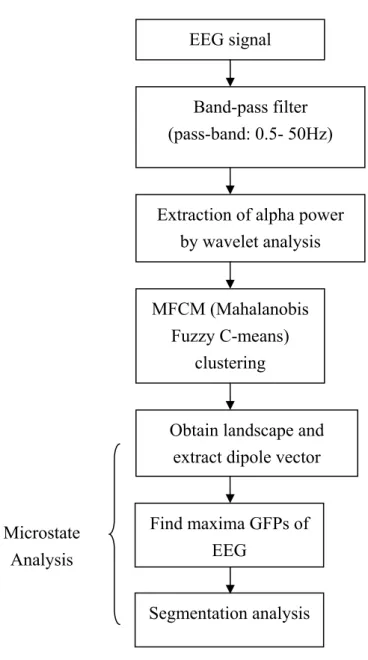
The entire scheme applied in this study is illustrated in Figure 2. This block diagram describes the whole scheme correlating different theories and methods to accomplish our aim of characterizing the multi-channel EEG spatial behaviors. Following this flowchart, details of theories and methods will be introduced. To quantify alpha power, we applied wavelet

analysis to 2-second windowed segments. Based on the block diagram in Figure 2, we then present the detailed concept and mathematics of each method in the following sections.

Firstly, EEG signals were pre-filtered by a band-pass filter with pass band 0.5 – 50 Hz. In the next step, wavelet analysis was applied to each 2-second EEG epoch to decompose raw EEG into characteristic rhythmic patterns. The epoch was identified to be alpha-dominated if the alpha power was at least 50% the total EEG power.

In MFCM (Mahalanobis Fuzzy C-means) clustering, we must find the initial cluster centers first. This study applied FCM for the determination of the initial centers. Difference between MFCM and FCM is that the correlation of data is adopted in MFCM’s computation, and distance computation is related to the distribution of data. In some case of clusters that cannot be line-separated, but it could be work in MFCM. In microstate analysis, wavelet transform was applied to 131ms-windowed EEG that approximately enclosed the longest alpha-wave epoch. Because of we went to analysis the mini-second’s brain state, so the window would not too bigger and not too to extract the alpha-power.

Figure 2 Flowchart of the entire scheme.

II.2 Alpha Wave Detection

For researching the effects of the alpha-wave, it is important to make sure that a trail of EEG is alpha dominate. We use wavelet transform toextract the wavelet coefficients of α, β, γ, δ, θ waves, and reconstructed them to calculate the α, β, γ, δ, θ power. Eq. (1), defines ρ as

EEG signal

Band-pass filter (pass-band: 0.5- 50Hz)

Extraction of alpha power by wavelet analysis

MFCM (Mahalanobis Fuzzy C-means)

clustering

Segmentation analysis Obtain landscape and

extract dipole vector

Find maxima GFPs of EEG

Microstate Analysis

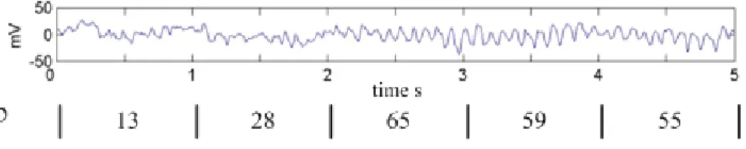
the percentage of α power to the total power. If ρ >=50% we call the EEG is alpha dominate. 100% p p p p p p α α β γ δ θ ρ= × + + + + (1)

Figure 3 plots a 5-second EEG signal. We computed the ρ value for each 1-second epoch. It is obviously that the signal is alpha dominated whenρ>=50%; while the epochs with 50%ρ< have no alpha rhythm. This example clearly demonstrates that ρ-criterion method allows us to detect alpha successfully. To deal with 30-channel EEGs, we identifies a given segment to be alpha dominated if anyone channel satisfies the ρ-criterion.

Figure 3 Alpha detection: the session with ρ>=50%is defined as alpha dominated.

II.3 Mahalanobis Fuzzy C-Means (MFCM)

Techniques based on the measurement of distances between quantitative features or attributes commonly apply such distance measures like Euclidean distance (ED) and

Mahalanobis distance (MD). Both distances can be calculated either in the original variable space or in the principal component (PC) space. The ED is easy to compute and interpret, yet, this is not the case for the MD. Nevertheless, MD provides better results of feature clustering because it measures the correlations between variables[14,15]. In a sense, MD can be used to

determine the degree of similarity of an unknown variable to the known one. It differs from Euclidean distance in that it takes into account the correlations of the data and is

scale-invariant, that is, independent of the scale of measurements.

Fuzzy c-means (FCM) is a fuzzy classifier based on the cluster means. Instead of

reaching a crispy decision like “0/1”, “true/false”, or “yes/no”, fuzzy allows the degree of truth of a statement ranging between 0 and 1. It is more suitable and feasible for classification and analysis of most empirical biomedical data. In this study, we employed MD distance

measurement in the membership value of FCM and compared the difference of classification results with or without correlation computation.

II.3.1 Mahalanobis Distance

The correlation is calculated from the inverse of the variance-covariance matrix of the data. However, the computation of variance-covariance matrix could cause problems. When the empirical data are measured over a large number of variables (for example, channels), they may contain a large amount of redundant or correlated information. The resulting variance-covariance matrix may become a singular or nearly singular matrix that can not be inversed.

In the case of object-i with 30 dimensional map xi =

(

µ µi1, i2,Lµi30

)

, the ED with

regard to the center map can be calculated for each object. Assume totally N objects, ED for object-i is computed as 2 2 2 1 2 30 1 2 30 ( ) ( ) ( ) i i i i ED = µ −µ + µ −µ +_L µ −µ for i = 1 to N, (2)

Where µ_i1to µ_i30are the variables of object-i, µ₁and µ are the means the variables of ₃₀ center objects.

To be able to compute the MD, first the variance-covariance matrix C is calculated: _x

1 ( ) ( ) ( 1) T x c c C X X N = − , (3) where the X is the data matrix containing N objects in the rows, X is the data matrix _c

X subtracted by the variable means X ; X_c =

(

X −X

)

. For the 30 dimensional map, X

can be defined as : 1,1 1,2 1,30 2,1 2,2 2,30 ,1 ,2 ,30 N N N X µ µ µ µ µ µ µ µ µ       =_{ }     L M O M L N subjects. (4)

The MD for object-i x is then _i

1

( ) ( )T

i i x i

MD = x −x C− x −x (5)

where x is the center of the data.

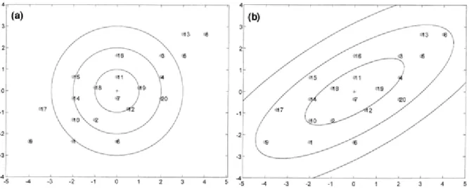
Figure 4(a) plots the simulated data for two variables µ₁ and µ₂ together with the circles representing the equal EDs with regard to the center point. Figure 4(b) plots the

simulated data for two variables µ₁ and µ₂ together with the ellipses representing the equal MDs with regard to the center point. This example illustrates the effect of taking into account the variance-covariance matrix of the data points.

Figure 4 The distances to the center of the data, (a) with the circles representing the equal EDs, (b) with the ellipses representing the equal MDs.

II.3.2 Mahalanobis Fuzzy C-Means Algorithm

The fuzzy-based classification algorism was improved by the scheme of c-means. By proper design of the membership function, we may improve the performance of classification. FCM (Fuzzy c-means) is different from c-means. Method of c-means performs poorly when the data set is fuzzy.

In this study, we employed the Mahalanobis FCM algorithm. Mahalanobis FCM algorithm evaluates the MD instead of ED in the membership-function construction. To introduce Mahalanobis FCM, we firstly summarize the parameters and variables in Table 1.

Parameters

c number of clusters

ch

n the variable’s degree

D setting number of iterations

ε allowed deviation

β exponent weight

N the number of objects

k the computing iteration

{

i|1

}

X = x ≤ ≤i N input data matrix, with every row is an object.

i

X data matrix belonging to ith _class

{ }

0 i0 ,1 Y = y ≤ ≤i c initial centers Outputs

{ }

_i ,1 Y = y ≤ ≤i c centers

( )

χ_iy ,1≤ ≤i c,1≤ ≤j N membership value

The strategy of Mahalanobis FCM analysis is described below. Step1：

Initialization: k =0,y_i,0 = y_i0, 1 i c≤ ≤

Step2：

Calculate the variance-covariance matrix and the MDs from data to centers _, 1 ( _, ) ( _, ) ( 1) T i k i k i k C X X N = − , 1 i c≤ ≤ and 1 j N≤ ≤ (6) 1 , ( , ) , ( , ) T ij k j i k i k j i k d = x −y C− x −y , 1 i c≤ ≤ and 1 j N≤ ≤ (7) Step3：

Compute the membership value

1 2 1 , , 1 , c ij k ij k l lj k d d β χ − − =       =_ _ _{ }      

∑

, 1 i c≤ ≤ and 1 j N≤ ≤ . (8) If l= and l₀ 0 , 0 l j k d = , we let 0 , l j k χ =1, χ_{ij k,} =0 (i≠ ) l₀ Step4：

Compute the new centers by,

, 1 , 1 , 1 N ij k j j i k N ij k j x y χ χ = + = =

∑

∑

(9) Step5： If 1 2 2 , 1 , 1 c i k i k i y ₊ y ε =   − <   

∑

 , let y_i =y_{i k, +1}, 1 i c≤ ≤ ; χ_ij =χ_{ij k,} , 1 i c≤ ≤ and 1 j N≤ ≤ .

Terminate the iteration. Step6：

If k<D, update the counter k= +k 1, repeat Steps 2 to 6.

Since the data have not been classified in the first run of iteration, X are not ready at _i

the step 2. We thus need to initialize the values of X . Note that the resulted output may vary _i

with the initial centers. Previous research showed that the initial centers significantly affected the output. In addition, we developed the scheme of estimating the initial centers by FCM and conducting feature clustering by Mahalanobis FCM.

II.3.3 The number of clusters

Beginning the clustering we should set the clustering numbers, and this number is decided by the correlation coefficients of the centers of clusters; when an correlation coefficients larger than θ that it indicates two cluster are similar, then the number will subtracted by one. So the initial number of clusters should be large. And in the past of our group’s researches, we decided the θ =0.3 as an suitable number, the cluster could be distinguished in this situation.

II.4 Brain Spatial Microstates

Researcher have disclosed changes of alpha power in each cerebral-cortex region under different states. These studies show that spontaneous alpha exhibits different distributions owing to the variation of alpha sources or the propagation ways. Most substantially, alpha distribution might be related to the states of alertness. In these studies, alpha power was

calculated by short-time spectral analysis based on Fourier-transformation method within a specific time window. Notice that Fourier approach is restricted by the piecewise stationary property that requires a narrow window of analysis and the frequency resolution that desires a wide window. In general, the window width is in the range from 1 to 5 seconds. However, from the viewpoint of the microscopic neural activities, the message is transmitted on the time scale of mini-second. The traditional FFT method is restricted to the window length and is difficult to explore the cerebral microstate.

In the research of Lehmann [16,17], he considered that the consistent neural activities would results in higher Global Field Power (GFP). The GFP is defined as the sum of the powers of all recoding channels at a specific sampling moment. The activity of each neuron could be considered as an electrical dipole vector including magnitude and direction. If each vector is uncorrelated with others, the activities would be canceled each other. In some conditions, neurons are driven by the same source that leads to a large GFP. As larger GFP often infers better signal-to-noise ratio (SNR), the driven response can be more significant with less noise interference. The appearance of local maximal GFP’s is thus an appropriate reference for choosing representative brain mappings (landscapes) to be utilized in the spatial microstate analysis. The sites of extremes (maximum and minimum) of a particular brain mapping compose a current dipole model generating the brain potential distribution recorded on the scalp.

continuous time duration within which the electrode sites of maximal and minimal potential are almost immobile (staying in a small region). Alternatively speaking, dipole vectors within a segment are stationary in a sense. A spatial segmentation algorithm was developed to separate different segments of brain topographical activities. Each particular segment class contains brain mappings with two sites of extremes appearing most frequently at a given region. As a consequence, the method adopted in this thesis provides rather local and subtle temporal information which cannot be accessible based on conventional Fourier analysis.

Lehmann [16,17] used the raw EEG data (potentials on the recording sites) to extract the brain landscapes of interest. His method is not practicable for our aim on the analysis of alpha-rhythmic behaviors. We applied the alpha-power for the brain landscape for the microstate analyzing.

A number of approaches and methods have been developed to analyze the EEG signals in time, frequency, and spatial domains. A number of methods have been proposed to explore various EEG features, in either macroscopic or microscopic aspects. Each particular method calls for different lengths of EEG segments and different numbers of channels. In our study, we firstly performed feature clustering for 20 minutes EEG signals based on the spatial characteristics. Then those 4-second EEG epochs with particular topographic features were extracted for microstate analysis. We will demonstrate that, based on a short EEG epoch of only a few seconds, the microstates method provides a way of exploring the brain

II.4.1 Global Field Power (GFP)

Global field power (GFP) at a given time instant represents the summation of EEG powers of all channels at that particular time t. A high GFP stands for a potential distribution with many peaks and troughs. According to [18], brain mappings with maximal GFP’s normally have better SNR (signal-noise-ration) performance. Hence, GFP provides a reference for us to select the appropriate time instants for microstates analysis. Assume a series A represents the data of channel-_k k. GFP is a function of time as shown below:

1/ 2 2 1 1 ( ) ch ( ) n k k ch GFP i A i n =   =   

∑

 , (10)

Where i represents the time point of discrete time signal and n is number of channel. In _ch

this thesis, the n is defined as 30. _ch

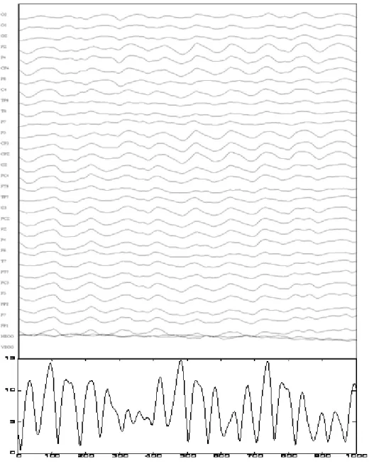
Figure 5 displays the GFP of a one-second EEG epoch. Apparently, GFP oscillates at a rhythm twice the EEG frequency due to the rectification effect.

Figure 5 The GFP of 1 second EEG epoch.

Since alpha activity was our major focus, we applied wavelet decomposition to raw EEG to extract alpha-band (8-12Hz) patterns before the GFP evaluation. As a consequence, we could reduce the contamination from other rhythmic bands, for example, delta (0-4Hz), theta (4-8Hz), and beta (>20Hz). We then computed the GFP of alpha-dominated EEG.

A brain microstate is defined as the constant landscape (brain topographical mapping) that lasts for a momentarily continuous time segment. The landscape was obtained by a 131msec moving window. Compute the power in the window and it results a 30 dimensional map. Note that we recorded 30-channel EEG in our experiment with a sampling rate of 1,000 Hz. Within a 4-second EEG epoch, we can obtain almost 4,000 maps. Previous study [18] has demonstrated that maximum GFP normally resulted in a good signal-to-noise ratio. This is accordingly a moderate clue for choosing the representative maps. We thus focused on the locations of extremes (maximum and minimum power value) of brain mappings.

In our study, brain microstates are characterized by the current dipole vector pointing from the minimum to the maximum potential of the multichannel EEG mapping on the scalp. As a consequence, it becomes important to determine the appropriate locations (EEG

channels) where extremes occur. Sometimes the extremes might be influenced by the noise. To deal with the noise problem, we developed an approach for better extracting the extremes.

First, we employed the spherical-coordinate model of the EEG electrodes to compute the average distance Dn between Cz and each of the rest 29 electrode sites. We then computed

the local average power (LAP) of brain potentials within the Dn-radius circle centered on each

channel. From the set of 30 local average powers (LAP’s), extremes (maximum and minimum) could be determined in a sense of better statistical significance. Finally, the centered electrode of maximal and minimal LAP forms the dipole vector of the brain microstate.

maxima) of GFP temporal sequence were selected for brain microstates analysis. These brain mappings were reduced to the locations of the extremes (maximum and minimum power value).

The so-called segment of a microstate begins with a particular brain potential map BPM1

characterized by a given dipole vector, and continues as long as the succeeding maps at the GFP peaks come up with the same dipole vector. That is, minimal and maximal LAP locates at the same sites as those of the beginning dipole vector obtained from BPM1. The segment

ends if the extreme LAP sites are out of range and continues if the sites are in the pre-defined range. The duration of a segment can be obtained straightforwardly. And the class of a

segment is defined by the extreme LAP sites whose have the highest occurrence times.

In each group, we analyzed four parameters: a) number of maximum GFPs per seconds, b) average duration of a segment, c) number of segments per second, and d) maximum

duration of the segments.

II.4.3 Selection of the Window of Extreme LAP Site

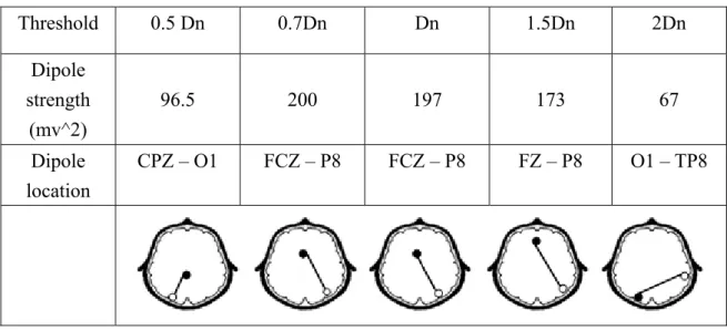
In the microstates analysis, we need to designate a circular window for justifying whether the extreme LAPs belong to the same microstate. Table 2 lists the results of an experimental subject with frontal alpha obtained by different threshold ( Dn : same as the Dn

before, ie, average of 29 distances from Cz to others). The threshold is used as the radius of the circular window.

A larger threshold could cause the different microstates as the same state, and on the other hand, a smaller threshold could separate one microstate into several segments. Either a small or a large threshold may not reliably reflect the evolution of microstates, so we had to find a suitable range for this threshold. According to our experiment, the threshold in the range of 0.7Dn ~ 1.5Dn provides obviously different dipole vectors with the range of 0.5Dn

and 2Dn ;while the locations of dipole vectors in range of 0.7Dn ~ 1.5Dn are about the same

as the frontal alpha, so it represent that the efficacy of segmentation are quiet the same in this region. Hence the threshold in this range (0.7Dn ~ 1.5Dn) is feasible. This study adopted Dn as

the threshold.

Table 2 Results of microstate analysis with different thresholds

Threshold 0.5 Dn 0.7Dn Dn 1.5Dn 2Dn Dipole strength (mv^2) 96.5 200 197 173 67 Dipole location CPZ – O1 FCZ – P8 FCZ – P8 FZ – P8 O1 – TP8

II.5 Experimental Protocol

As illustrated in Figure 6, the entire recording experiment involved three sessions: pre-, mid-, and post-meditation session for experimental subjects who have been practicing Chan meditation, and pre-, mid-, and post-relaxation session for control subjects that are normal,

healthy people within the same age range as the experimental subjects.

Figure 6 Experimental protocol.

In this study we selected eight healthy control subjects and eight healthy experiment subjects, and they were no medical or psychological disorders present.

III Experimental Results

Section III discusses the experimental results of this research study. The content is organized according to two main tasks conducted in the study: 1) EEG spatial feature analysis and classification, and 2) brain microstate analysis, which are presented in Sections III.1 and III.2, respectively.

Inter-subject and intra-subject variations of EEG signals are inevitable and significant. Brain spatial microstate is undoubtedly time-dependent. Hence it is important to select the epoch of interest from the long EEG record. We used the spatial (brain-mapping)

classification scheme to extract consecutive four-second epoch within the same class; and then analyzed the microstate of the epoch. This chapter presents the results of spatial

classification and microstate analysis.

III.1 Results of Brain-Mapping Classification

In this section, we report the results of classifying brain topographical mappings by Mahalanobis FCM. In addition, results are compared between experimental and control group. As mentioned in II.1, wavelet analysis was applied to each 2-second (pre-filtered by a

band-pass filter) EEG epoch to decompose raw EEG into characteristic rhythmic patterns. The epoch was identified to be alpha-dominated if the alpha power was at least 50% the total EEG power

III.1.1 Control Subjects

Figures 6 to 8 display the classification results of one representative subject (20040315) in the control group. The results were classified into three clusters (classes). Notice that the color charts reflect the associate cluster (Cluster 1, 2, or 3) identified at the time instant of the 2-sec window centering. The color charts thus display the temporal evolution of

Figure 6 Results of interpretation and classification of EEG brain mappings for a control subject in the pre-session background recording (before main session of relaxation).

Figure 8 Classification result of one control subject in the post-session recording.

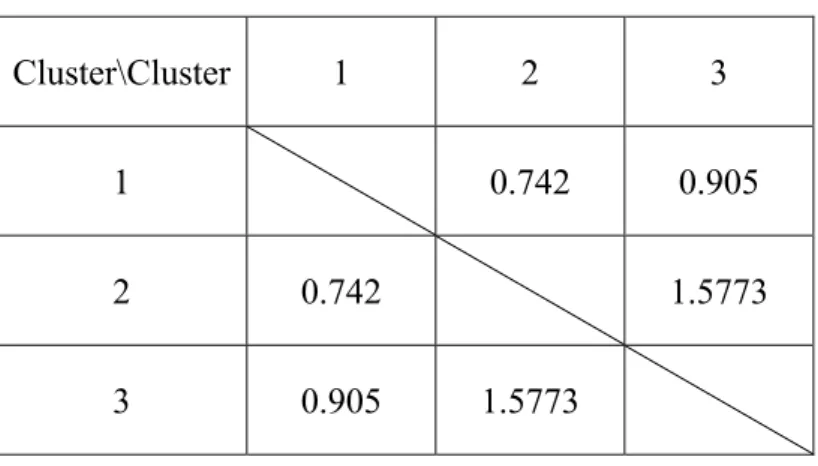
According to the results in Figures 6 to 8, all clusters derived contained no frontal-alpha activity for all the recording sessions. Very few control subjects had frontal alpha cluster. Table 3 shows the correlations between each pair of cluster centers. Table 4 lists the distance between each pair of cluster centers, while Table 5 lists the standard deviation of all members belonging to the same cluster. The inter-cluster distance were larger than the within-cluster standard deviation, justifying the effectiveness of this classification scheme.

Table 3 Correlations between clusters

1 1 -0.105 -0.585

2 -0.105 1 -0.745

3 -0.585 -0.745 1

Table 4 Distance between cluster centers

Cluster\Cluster 1 2 3

1 0.742 0.905

2 0.742 1.5773

3 0.905 1.5773

Table 5 Number of each cluster and standard deviation of cluster members

Cluster number Standard deviation

1 109 0.550

2 87 0.675

3 86 0.646

III.1.2 Experimental Subjects

Figures 9 to 11 display the interpretation and classification results of an experimental subject (20040306). Three clusters were derived. Same as previous figures, the color bar

charts display the temporal evolution of brain-mapping cluster.

Figure 9 Results of interpretation and classification of EEG brain mappings for an experimental subject in the pre-session background recording (before main session of meditation).

Figure 11 Classification result of an experimental subject in the post-session recording (after main session of mediation).

From Figures 9 to 11, alpha activities apparently moved toward the frontal regions for the meditation subject. In addition, frontal alpha increased in the meditation session that occupied approximately one-third record length of the main session. Table 6 shows the correlations between the three class centers, and Table 7 and 8 show the distance between centers and the standard deviation. The distances between centers are also larger than the standard deviation.

Table 6 Correlations between clusters

Cluster\Cluster 1 2 3

1 1 -0.620 -0.851

2 -0.620 1 0.116

3 -0.851 0.116 1

Table 7 Distance between cluster centers

Cluster\Cluster 1 2 3

1 0.938 1.390

2 0.938 0.624

3 1.390 0.624

Table 8 Number of each cluster and standard deviation of cluster members

Cluster number Standard deviation

1 55 0.603

2 57 0.632

3 55 0.525

III.2 Results of Microstate Analysis

features extracted by classification in previous sub-section. For the experimental group with Zen- meditation experience, four-second frontal alpha and occipital alpha were selected. However, control subjects in this study appeared to have rare frontal-alpha activity. We accordingly only analyzed the four-second occipital alpha for the control group.

III.2.1 Frontal-alpha and occipital-alpha microstate in experimental group

According to the results in Table 9 and Figure 12, average duration of the alpha brain microstate demonstrates that frontal alpha exhibits a longer, continuous average duration of microstate. Figure 13 displays the results of dipolar-vector representation for modeling frontal-alpha (FA) and occipital-alpha (OA) microstates. One phenomenon to be further investigated is that, FA (OA) dipoles might emerge in the regions other than frontal (occipital) area.

Table 9 Frontal-alpha (FA) and occipital alpha (OA) microstate analysis for experimental subjects (4-second epoch).

Subject 1 2 3 4 5 6 7 8 Mean S.D.

Number of maximum GFPs per second

FA 25 26.8 28.5 22.8 23 25.8 28.3 20.8 25.1 2.8

OA 27.5 26.5 27.5 26 28.5 24.8 29.8 23.3 26.7 2.1

Average duration of an alpha brain microstate (in ms)

FA 77.0 82.2 83.1 67.4 99.3 88.2 80.2 92.9 83.8 9.8

OA 63.9 88.7 64.5 70.0 77.5 70.2 58.0 79.3 71.5 9.9

Number of alpha brain microstates per second

FA 7 6 6 6 6 7 7 5 6.3 0.7

Maximum duration of an alpha brain microstate (in ms)

FA 198 251 237 221 251 242 197 172 221 29

OA 187 182 202 245 278 187 167 163 201 40

Figure 12 Average duration of brain microstate segments( frontal alpha and occipital alpha)

Figure 13 Dipolar vector model for alpha brain microstate with the filed minimum and maximum represented by circle and black dot, respectively.

III.2.2 Comparison of occipital-alpha microstates in experimental and control groups

The result of average duration of microstate for these two groups shows no obviously 0 20 40 60 80 100 1 2 3 4 5 6 7 8 me a n FA OA subject ms

difference (meditation subjects: 71.5; relax subjects: 68.4). Although the control group’s number of microstates is little larger, but its duration is less than experimental group. So we think there is no very difference between these two groups. Figure 15 shows the locations of the two extreme poles, because of the analyzing signal selection of these two group is occipital alpha, the most locations are match with the classification result.

Table 10 Microstate analysis of 4-second occipital alpha mappings for the experiment and control subjects.

Subject 1 2 3 4 5 6 7 8 Mean S.D.

Number of maximum GFPs per second

MD 28 27 28 26 29 25 30 23 26.7 1.9

Relax 22 25 26 27 24 27 25 27 25.3 1.7

Average duration of an alpha brain microstate (in ms)

MD 63.9 88.7 64.5 70.0 77.5 70.2 58.0 79.3 71.5 9.9

Relax 73.8 75.8 63.7 63.4 69.3 69.6 51.5 79.8 68.4 8.8 Number of alpha brain microstates per second

MD 7 7 7 7 5 6 9 6 6.6 1.0

Relax 6 6 7 8 6 7 7 5 6.3 0.8

Maximum duration of an alpha brain microstate (in ms)

MD 187 182 202 245 278 187 167 163 201 40

Figure 14 Average duration of brain microstate segments(mediation and relaxation)

Figure 15 Dipolar vector model for alpha brain microstate with the filed minimum and maximum represented by circle and black dot, respectively.

III.2.3 Results in different length of EEG

Since the research of microstates[18] used four seconds EEG for analysis, and the average duration of microstate are about 60~100 ms. So we interest that the analysis time can

0 10 20 30 40 50 60 70 80 90 1 2 3 4 5 6 7 8 me a n MD Relax subject ms

be reduced or not. Table 11 shows the results of microstate analysis in different length of EEG signal (2, 2.5, 3, 3.5, and 4 seconds) in frontal alpha and occipital alpha of experimental group. The result shows the same thing that the average duration of microstate in frontal alpha is longer than in occipital alpha.

Table 11 The microstate analysis results of 4-seconds EEG with the experiment subjects of frontal alpha (FA) and occipital alpha (OA)

Average duration of alpha brain microstate

Subject 1 2 3 4 5 6 7 8 Mean S.D. 2 seconds EEG FA 62.6 86 67 80.1 90.7 92.8 77.3 70.5 78.4 11.1 OA 57.7 104.5 60.1 67.5 77.5 84.8 73.4 70.8 74.6 15.0 2.5 seconds EEG FA 73.2 89.3 75.7 89.3 115.8 89.2 68.7 118.9 90.0 18.7 OA 41.2 77.6 51.2 66.8 63.3 69.8 66 72.1 63.5 11.8 3 seconds EEG FA 68.9 107.5 84.8 70.6 90.3 85.2 74.7 113.5 86.9 16.4 OA 63.5 64.1 64.0 65.2 73.2 57.4 79.3 95 70.2 12.1 3.5 seconds EEG FA 67.0 83.6 83.6 69.4 72.7 79.1 67.6 88.7 76.5 8.4 OA 72.8 75.2 58.0 64.5 65.0 70 83.9 84.6 71.8 9.4 4 seconds EEG FA 77.0 82.2 83.1 67.4 99.3 88.2 80.2 92.8 83.8 9.8 OA 63.9 88.7 64.5 70.0 77.5 70.2 58.0 79.3 71.5 9.9

III.2.4 Results in frontal alpha and occipital alpha of experimental group (only adopts

maximum power location of maps)

than 100 m-seconds, which is considered as a shorter duration of state. So we shown the dipoles( in maxima GFPs) in one minute (Figure 16). And we found that the location of minimum power changed frequently, the minimum power location is usually in the edge; but the values of power in the edge locations are very close, so we think the frequently changed location of minimum power cause the results of duration of alpha brain microstate shorter. Hence following shows the microstate results which the segment only adopts the maximum power location.

Figure 16 Dipoles appear in one minute follow by the time

Table 12 lists the results of experimental subjects of FA and OA, the average duration of an alpha brain microstate of FA is 208 m-sec that is longer than OA’s, and the maximum microstate duration is 517 m-sec also longer than OA’s. Table 13 shows the results between experimental subjects and control subjects (occipital alpha); the difference of results is not

obviously. Figures 17 and 18 plot the maximum poles locations, and it generally matches with the brain mappings.

Table 12 The microstate analysis results of 4-seconds EEG with the experiment subjects of frontal alpha (FA) and occipital alpha (OA) with only maximum power adopted

Subject 1 2 3 4 5 6 7 8 Mean S.D.

Number of maximum GFPs per second

FA 25 27 23 25 24 25 27 22 25 1.7

OA 25 26 25 24 23 26 28 23 25 1.7

Average duration of an alpha brain microstate (in ms)

FA 206 148 234 328 219 172 145 195 208 59

OA 168 115 197 226 167 199 142 193 175 35

Number of alpha brain microstates per second

FA 4 5 3 3 3 6 3 4 4 1.1

OA 4 6 4 4 5 4 5 4 5 0.8

Maximum duration of an alpha brain microstate (in ms)

FA 474 393 524 767 736 397 350 492 517 156

OA 451 318 597 576 348 550 394 580 477 113

Table 13 The microstate analysis results of 4-seconds EEG with the experiment subjects of mediation (MD) and control subjects of relaxation (Relax) with only maximum power adopted

Subject 1 2 3 4 5 6 7 8 Mean S.D.

Number of maximum GFPs per second

MD 25 26 25 24 23 26 28 23 25 1.7

Relax 26 26 24 25 25 27 26 27 26 1.1

Average duration of an alpha brain microstate (in ms)

MD 168 115 197 226 167 199 142 193 175 35

Relax 193 126 165 234 152 215 129 138 169 41 Number of alpha brain microstates per second

MD 4 6 4 4 5 4 5 4 5 0.8

Relax 5 5 5 4 4 4 5 6 5 0.7

Maximum duration of an alpha brain microstate (in ms)

MD 451 318 597 576 348 550 394 580 477 113

Relax 497 249 388 455 502 475 511 379 432 89

Figure 18 Maximal polarities for experimental subjects in mediation (MD) and control subjects in relaxation.

IV. CONCLUSION AND DISCUSSION

characteristics of various alpha rhythms down to the micro-second portrait, instead of the long-time property. In our findings, experimental subjects apparently exhibited more frontal alpha than control subjects. Preliminary results are summarized as follows. Firstly, average duration of the alpha-microstate segment is longer in frontal alpha than in occipital alpha. Second, the number of segments (the occipital alpha state shows more segments than does frontal alpha). And third, the minimum poles of dipole vectors make the average duration shorter. In the case, we need to discard those small poles in order to derive a reasonable estimate of the microstates duration.

We proposed a clustering method for the alpha brain maps classification which has been

demonstrated to perform effectively. The classification results tend to be classified into frontal, central and occipital maps for the alpha microstate analysis. The results of microstate analysis reveal significant difference between the frontal-alpha and occipital-alpha groups in

mediation. Longer duration of alpha microstate occurs in the frontal-alpha group. In fact, researches have shown that, in mediation, the region of frontal cortex is related to the hormone modulated [29]. In addition, more stable alpha brain was reported for such kind of reaction.

Brain microstate analysis can be extended to the exploration of other EEG features. Although current study was focused on alpha dipolar-vector model, it is an important and appealing issue on the variations of alpha rhythmic compositions based on multi-resolution spectral analysis. The phenomenon might be correlated with brain oscillatory model of alpha

rhythms. Then, the further step may be taken to investigate the spatio-spectral microstate of alpha brain either during Chan meditation or at normal relaxation.

References

[1] T. Kalayci and Ö. Özdamar, “Wavelet preprocessing for automated neural network detection of EEG spikes,” IEEE Eng. Med. Biol. M, vol. 14, no. 2, pp. 160–166, 1995. [2] R. Cooper, J. W. Osselton, and J. C. Shaw, EEG Technology, 3rd ed. Woburn, MA:

Butterworth, 1980.

[3] K. Ansari-Asl, J.J. Bellanger, F. Bartolomei, F. Wendling and L. Senhadji, “Time-Frequency Characterization of Interdependencies in Nonstationary Signals: Application to Epileptic EEG,” IEEE Transactions on Biomedical Engineering, vol. 52, no. 7, pp. 1218-1226, Jul. 2005.

[4] N. Acır and M. Kuntalp, “Automatic Detection of Epileptiform Events in EEG by a Three-Stage procedure Based on Artificial Neural Networks,” IEEE Transactions on

Biomedical Engineering, vol. 52, no. 1, pp. 30-40, Jan. 2005.

[5] E.ST. Louis and E. Lansky, “Meditation and epilepsy: A still hung jury,” Medical

Hypotheses, vol. 67, issue 2, pp. 247-250, Apr. 2006.

[6] C. Babiloni, G. Frisoni and M. Steriade, “Frontal white matter volume and delta EEG sources negatively correlate in awake subjects with mild cognitive impairment and Alzheimer's disease,” Clinical Neurophysiology, vol. 117, pp. 1113–1129, Jan. 2006. [7] O.L. Carter, D.E. Presti and C. callistmon, “Meditation alters perceptual rivalry in

Tibetan Buddhist monks,” Current Biology, vol. 15, no.11, pp. 412-413, 2005.

[8] S.W. Lazar, C.E. Kerr and R.H. Wassermana, “Meditation experience is associated with increased cortical thickness,” Neuroreport, vol. 16, no. 17, pp.1893–1897, Nov. 2005. [9] D.A. Lindberg, “Integrative Review of Research Related to Meditation, Spirituality, and

the Elderly,” Geriatric Nursing, vol. 26, no. 6, 2005.

[10] R.C. Shetty, “Meditation and its implications in non pharmacological management of stress related emotions and cognitions,” medical hypotheses, pp. 1198-1199, 2005. [11] M.J. Ott and Rebecca L. Norris, “Mindfulness Meditation for Oncology Patients: A

Discussion and Critical Review,” Integr Cancer Therapies, vol. 5, no. 2, pp. 98-108, 2006. [12] L.S. John, Biosignal and Biomedical Image Processing. MARCEL DEKKER , 2004,

pp. 149.

[13] I. Daubechies, Ten lectures on wavelets. Philadelphia, PA: SIAM, 1992. [14] A.R. de Leona and K.C. Carrière, “A generalized Mahalanobis distance for mixed

data,” Journal of Multivariate Analysis, vol. 92, issue 1, pp. 174-185, Jan. 2005. [15] R.D. Maesschalck, D.J. Rimbaud and D.L. Massart, “The Mahalanobis distance,”

Chemometrics and Intelligent Laboratory Systems, vol. 50, Issue 1, pp. 1-18, Jan. 2000.

[16] D. Lehmann and T. Koenig, “Spatio-temporal dynamics of alpha brain electric fields, and cognitive modes,” International Journal of Psychophysiology, vol. 26, pp. 99-112, 1997.

[17] D. Lehmann, “Multichannel topography of human alpha EEG fields,”

Electroencephalogr Clin Neurophysiol, vol. 31, no. 5, pp. 439-49, Nov. 1971.

[18] J.L. Cantero, M. Atienza, R.M. Salas and C. Gomez, “Brain Spatial Microstates of Human Spontaneous Alpha Activity in Related Wakefulness, Drowsiness Period, and REM Sleep,” Brain Topography, vol. 11, no. 4, pp. 257-263, Jun. 1999.

[19] B. S. Oken and K.H. Chiappa, “Statistical issues concerning computerized analysis of brainwave topography,” Annals of Neurology, vol. 19, issue 5, pp. 493-497, May 1986.

[20] SE. Lukas, JH. Mendelson, BT. Woods, NK. Mello and SK. Teoh, “Topographic distribution of EEG alpha activity during ethanol-induced intoxication in women,”

Journals of Studies on Alcohol, vol. 50, pp. 176-85, Mar. 1989.

[21] J. Zeitlhofer, P. Anderer, S. Obergottsberger, P. Schimicek, S. Lurger, E. Marschnigg, B. Saletu and L. Deecke1, “Topographic mapping of EEG during sleep,” Springer

Netherland, vol. 6, no. 2, pp. 123-129, Mar. 1993.

[22] J.L. Cantero, M. Atienza, C. Gomez, “Spectral Structure and Brain Mapping of Human Alpha Activities in Different Arousal States,” Neuropsychobiology, vol. 39, pp. 110-116, 1999.

[23] G. Bush, P. Luu and M.I Posner., “Cognitive and emotional influences in anterior cingulate cortex,” Trends in Cognitive Sciences, vol. 4, pp. 215-222, 2000.

[24] C.R. Maclean, K.G. Walton, S.R. Wenneberg, D.K Levitsky, J.P. Mandarino, R. Waziri, S.L. Hills, R.H. Schneider, “Effect of the Transcendental Meditation program on adaptive mechanicsm: changes in hormone levels and responses to stresss after 4 months of practice,” Psychoneuroendocrinology, vol. 22, pp. 277-295, 1997.

[25] D.N. Pandya and B. Seltzer, “Association areas of cerebral cortex,” Trends in

Neuroscience, vol. 5, pp. 386-390, 1982.

Klein, K. Hazen, W.J Bunney, J.H. Fallon and D. Keator, “Prediction of antidepressant effect of sleep deprivation by metabolic rates in the ventral anterior cingulated and medical prefrontal cortex,” The American Journal of Psychiatry, vol. 156, pp. 1149-1158, 1999.

[27] K.L. Phan, S.F. Taylor, R.C. Welsh, L.R. decker, D.C. Noll, T.E. Nichols, J.C. Britton, I. Liberzon, “Active of the medical prefrontal cortex and extended amygdale by individual ratings of emotional arousal: a fMRI study,” Biological Psychiatry, vol. 53, pp. 211-215, 2003.

[28] K.N. Ochsner, J.J. Gross, “The cognitive control of emotion,” Trends in Cognitive

Sciences, vol. 9, pp. 242-249, 2005.

[29] S. Yamamoto, Y. Kitamura, N. Yamada, Y. Nakashima, S. Kuroda, “Medial Prefrontal Cortex and Anterior Cingulate Cortex in the Generation of Alpha Activity Induced by Transcendental Meditation: A Magnetoencephalographic Study, Acta Medica

Report for the academic trip to Beijing and Baoding from July 8 to

July 15, 2009

In this trip, I have accomplished two important tasks:

1. participation in the International Conference of Machine Learning and Cybernetics (ICMLC 2009) held in Baoding, Hebei (July 12‐15), and

2. successful establishment of Cross‐Strait Cultural/Educational relationships between National Chiao Tung University in Hsinchu and most well‐known, top‐ranked universities in Beijing (北交大、北大、北清華、北理工、北航、北郵).

In the conference ICMLC 2009, my paper “Microstate analysis of alpha‐event brain topography during chan meditation” was recommended to compete for the Best paper award. I accordingly reported my paper in two sessions, ICMLC and ICWAPR Best Paper Award Session and Fuzzy Set Theories and Methods (II) Session in which I played the role of session moderator.

MICROSTATE ANALYSIS OF ALPHA-EVENT BRAIN TOPOGRAPHY

DURING CHAN MEDITATION

PEI-CHEN LO1_{, QIANG ZHU}2

1 _{Department of Electrical and Control Engineering, National Chiao Tung University, Hsinchu 30010 Taiwan} 2_{School of Computer & Information Technology, Beijing Jiaotong University, Beijing, 100044 China}

E-MAIL: [email protected]; [email protected]

Abstract:

This paper reports our preliminary result of microstate analysis for the spatiotemporal characteristics of Chan-meditation brain wave (electroencephalograph, EEG)

based on time-varying dipolar-vector model of the α-map.

Microstate behavior reveals subtle transience of focalized event. Multi-channel α-event epochs were identified by Wavelet decomposition and feature extraction. Global field

power was adopted as the criterion to choose α-map

candidates (normalized α-power vectors), that were further classified by Mahalanobis Fuzzy C-means into different region-focalization states. Transition between various α-event

focalization states was ready to be explored via microstate analysis. Our findings reveal that Chan-meditation

practitioners exhibit longer duration of frontal α-event

microstate, reflecting sustained stability of the brain generators.

Keywords:

Microstate analysis; electroencephalograph (EEG); Chan meditation; wavelet decomposition; Mahalanobis Fuzzy C-means (M-FCM); brain mapping; frontal alpha.

1. Introduction

For decades, scientific exploration on meditation benefits has corroborated the effectiveness of meditation practice on the health promotion, hypertension treatment, anti-aging, hormone-level regulation, stress manipulation, anxiety reduction, etc. [1], [2]. In the course of Chan meditation, practitioners experience various states of consciousness, according to their subjective narration, that transcends the physiological (the fifth), mental (the sixth), subconscious (the seventh), and Alaya (the eighth) conscious state, and eventually reaches the spiritual realm. EEG measuring thus has been intensively studied to explore the underlying brain physiological changes correlating to various states of consciousness during meditation. Numerous studies have been conducted since 1960s [3]–[7]. Although the neuro-electrophysiological correlation of

meditation-elicited consciousness state is still an open question, the predominant EEG findings in most meditation techniques have implicated the increase in theta- and alpha-band power and the decrease at least in alpha frequency [2], [5], [7].

In the field of EEG study, the spatial or topographical features provide an access to the detection of focal EEG phenomena that have a relationship to focal pathology or brain dynamic origin [8]-[10]. The spatial distribution of EEG features over the scalp surface, often called the EEG

mapping or the brain mapping, offers a quickly pictorial

assessment of possible event focalization. Such graphical display provides an easy and straightforward aid to visual inspection of focal activities in clinical diagnosis, yet, cannot resolve stable-to-transient behaviors of the focal source.

According to our study on Chan-meditation EEG during the past decade, a number of EEG characteristics have been found to be evidently linked to the Chan-meditation practice [11]-[13]. We have reported our findings on frontal alpha activity and beta-dominated phenomena, mainly from the temporal and spectral aspects. This work was particularly focused on subtle behaviors of spatiotemporal shifting of EEG α-event focalization during Chan meditation, based on the concept of spatial microstate analysis.

2. Theory and Method

The EEG content is generally interpreted according to the frequency ranges that include δ-wave (0~4Hz), θ-wave (4~8Hz), α-wave (8~13Hz), β-wave (13~30Hz), and γ (30~70Hz). Researches during the past several decades have disclosed the phenomenon that particular EEG patterns correlated closely with some physiological, mental, or emotional states. For instance, occipital α-wave becomes dominant during the eye-closed relaxation; while frontal α-wave characterizes a certain stage of inward-attention

mindfulness during Chan meditation.

2.1. Experimental setup and protocol

This study utilized the 30-channel recording montage shown in Figure 1. C4 T8 FCz Fz C3 T7 CPz Pz Oz Cz FP2 F4 F8 FC4 FT8 FP1 F3 F7 FC3 FT7 O1 P3 P7 CP3 TP7 O2 P4 P8 CP4 _TP8 C4 T8 FCz Fz C3 T7 CPz Pz Oz Cz FP2 F4 F8 FC4 FT8 FP1 F3 F7 FC3 FT7 O1 P3 P7 CP3 TP7 O2 P4 P8 CP4 _TP8

Figure 1. The 30-channel EEG recording montage Reference electrode was the linked mastoid MS1-MS2. EEG signals were pre-filtered by a band-pass filter with pass band 0.5 – 50 Hz (sampling rate 200Hz). We compared the α-wave microstates of two groups of subjects, 8 Chan-meditation practitioners (experimental group) and 8 normal, healthy subjects without any meditation experience (control group)

The scheme of α-wave microstate analysis can be briefly described by the procedure below:

EEGÆ Pre-process by bandpass filtering (0.5-50Hz)Æ Estimate α-power by Wavelet analysisÆ M-FCM clusteringÆ Derive landscape and corresponding dipole vectorÆ Microstates analysis. Experimental Protocol involves three sessions (Figure 2), pre-, mid-, and post-meditation (relaxation) session for experimental (control) subjects.

Figure 2. Experimental protocol

2.2. Wavelet analysis for α-power estimation

According to our previous studies [11]-[13], EEG epoch of 2 seconds is appropriate for identifying a typical

EEG rhythm based on wavelet analysis. Frontal alpha was highly correlated with a specific meditation state. We thus began with the analysis of frontal-alpha brain microstates. To identify the emergence of frontal-alpha activities, we applied wavelet transform to extracting the wavelet coefficients of α, β, γ, δ, and θ waves and then calculating their powers after reconstructing each particular EEG rhythm [12]. Next, the α-dominated epochs can be extracted by the criterion ρ≥50%, where ρ is the percentage of α power to the total power:

100% p p p p p p α α β γ δ θ ρ= × + + + + (1)

In this study, an α-dominated epoch only requires at least one channel satisfying the _ρ-criterion.

2.3. Mahalanobis fuzzy C-means (M-FCM)

After temporal searching for α-dominated EEG epochs (denoted by map xi), we developed the pattern recognition

scheme, based on fuzzy c-means, to cluster the alpha activities into frontal-, parietal-, and occipital-alpha segments. And we analyzed the frontal and occipital α-wave microstates in Chan-meditation as well as the occipital and parietal α-wave microstates in relaxation.

Fuzzy c-means (FCM) is a fuzzy classifier based on the cluster means. Instead of reaching a crispy decision like “0/1” or “true/false”, fuzzy allows the degree of truth of a statement to range between 0 and 1. It is more suitable and feasible for classifying and analyzing the biomedical data. In this study, we employed MD (Mahalanobis Distance) measurement, instead of Euclidean distance (ED), in the FCM membership function reconstruction [14]. In feature clustering based on FCM, MD is superior to ED in the aspect that MD takes into account the correlations of the data set and is scale-invariant.

Consider xi = (μi1, μi2, …μi30) as the ith sample of

totally N 30-channel α-dominated brain mappings (briefly, α-map) extracted by ρ-criterion. MD distance is computed by

(

) (

)

T i x i i x X C x X MD = − −1 − ₍₂₎

where X is the average map of the N α-map samples, Cx

is the variance-covariance matrix calculated by

( ) ( )

c T c x X X N C ) 1 ( 1 − = (3)

The centralized data matrix is Xc=(X−X ) where X is an

20-minute EEG.

FCM clustering requires the determination of cluster number (c) in advance. Starting from a large value of c, we computed the correlation coefficients of the cluster centers. Two clusters are identified to be similar and merged together when the correlation coefficient is larger than a given threshold _θ. Empirical value of _θ=0.3 provides satisfactory result of clustering.

2.4. Alpha-map spatial microstates

To investigate the spatial behaviors of event (α-map) localization of Chan-meditation brain dynamics, we examined the temporal steadiness-versus-transience of focal source on a 4-second basis. The concept of microstate analysis provides a medium of exploring subtle evolution of focal event that might reveal microscopic mechanisms of brain dynamics accounting for transcendental state of Chan meditation.

Distribution of brain potentials is modeled by a 4-dimensional function of time (t) and space (x, y, z). Construction of focal source highly depends on selection of time instant. According to Lehmann [15], consistent neural activities would result in higher global field power (GFP). The GFP is defined as the sum of the powers of all EEG recoding sites at a specific time. A large GFP often infers significant dipolar focalization and, evidently, promises better signal-to-noise ratio (SNR) performance. The appearance of temporally local maximal GFP is thus an appropriate reference for choosing representative brain mappings (landscapes) for the spatial microstate analysis. The sites of extremes (maximum and minimum) of a particular brain mapping compose a current dipole model generating the brain potential distribution recorded on the scalp. Let Ak denote the EEG potential at channel-k and nch

be the number of channel. GFP evaluated at time instant i is:

∑

= = nch k k ch i A n i GFP 1 2_{( )} 1 ) ( (4)

Brain microstate is defined as the constant landscape (brain-potential topographical mapping) that lasts for a momentarily continuous time segment. In our study, the landscape was obtained by a 131msec moving window that approximately enclosed the longest α-wave epoch. To characterize the particular microstate, the current-dipole vector, pointing from the minimal to the maximal potential, was derived from the landscape. To avoid the effect of noise contamination, electrodes of extremes were determined as follows.First, distance Dn was computed by averaging all

the inter-distances between Cz and each of the rest 29

electrode sites. We then computed the local average potential (LAP) of EEG potentials within the radius-Dn

circular region centered on each channel. The extremes were finally determined from the set of 30 LAP values. The centered electrodes of maximal and minimal LAP form the dipole vector of the brain microstate.

To quantify the transient against stationary behaviors of α-microstates, we define the segment of a microstate as the time duration of a particular focalized event (current-dipole vector) that produces consistent brain-potential mappings. The segment continues if the extreme LAP sites are in the pre-defined range and ends if the sites are out of range. Note that each segment may belong to a particular class defined by the extreme LAP sites. Within the same group, four parameters were derived: a) number of maximum GFP peaks, b) average duration of the segment, c) number of segments per second, and d) maximum duration of the segments.

3. Results

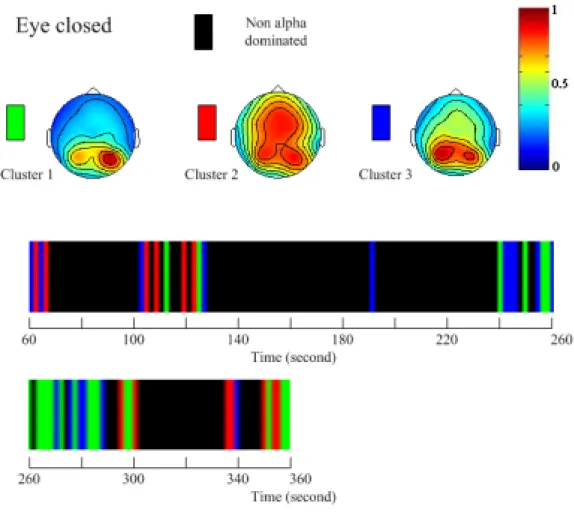
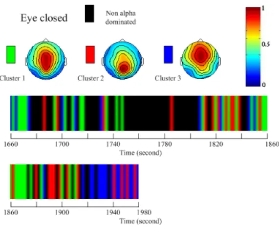
Based on wavelet decomposition and M-FCM, EEG spatial features were analyzed and the extracted α-maps were classified into three clusters. Figure 3 displays three clusters derived from the α-maps of one experimental subject, including occipital, parietal, and frontal α-maps (denoted by αO, αP, and αF).

Figure 3. Classification result of one experimental subject (in main session) and 10-min temporal evolution of different α-map clusters.

In the beginning 3-min meditation, occipital and parietal α maps interweaved. After a particular α-blank mindful attention in the mid 3-min, α-event was found to propagate toward frontal region at the end of the 10-min course.

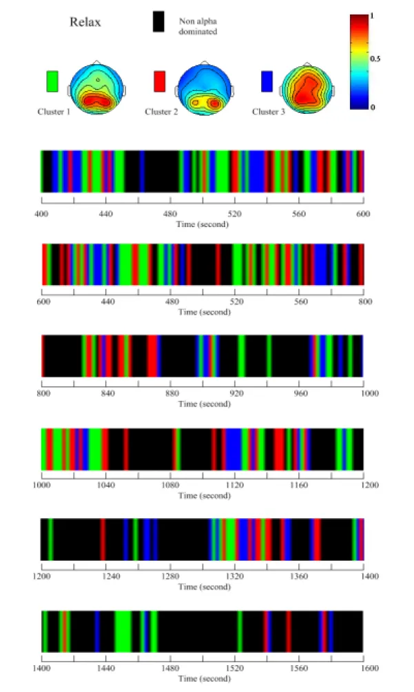
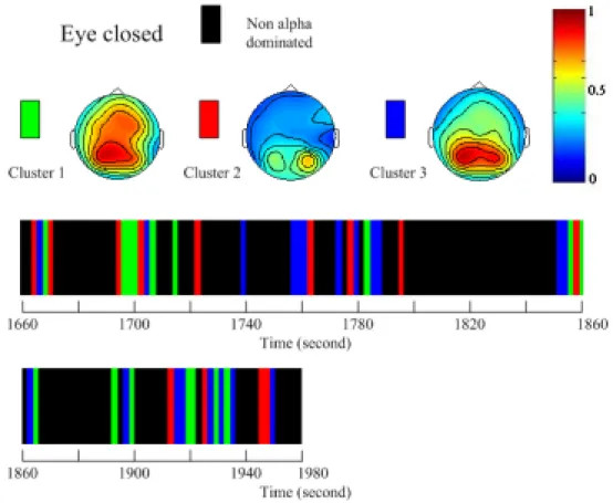
Note that, in control group, three α-map clusters contain mainly the occipital and centro-parietal α-maps (denoted by αO and αCP), as shown in Figure 4, with frontal

α-maps (αF) diminishing.

Figure 4. Classification result of one control subject (in main session) and 5-min temporal evolution of different α-map clusters.

Microstate analysis for α-event demonstrates that, in the experimental group, frontal α-event persists longer than occipital α-event (average segment length is 89.8ms for αF

and 71.5ms for αO, while maximum segment length is

221ms for αF and 201ms for αO).

Figure 5 displays the 1-min temporal evolution of α-event dipole vector, pointing from minimum (०) to maximum (•). Apparently, αF and αO dipoles might

originate in the regions other than frontal (occipital) area. Subtle transience of αF and αO microstates was clearly

explored in this scheme.

4. Conclusions

This paper presents a novel approach for exploring the spatial-temporal characteristics of various α-maps down to the milli-second portrait, instead of long-time trend. Wavelet analysis and M-FCM successfully extracted and classified various α-maps. Experimental subjects

apparently exhibited more frontal alpha αF than control

subjects. In Chan-meditation EEG results, average duration of the α-map microstate segment is longer in frontal alpha than in occipital alpha.

Figure 5. Dipolar vector evolution for α-event Results of microstate analysis revealed the difference of αF group and αO group in mediation. Longer duration of

microstate occurs in αF, instead of αO. This might be an

evidence correlating to the neuro-physiological state of meditation that involves the region of frontal cortex relating to the hormone modulated. Furthermore, sustained stability of α-event with this reaction may infer the state of less information processing. Consistent increase of frontal alpha can be recognized as the major distinction between meditation and relaxation. At this stage of meditation, according to meditators’ narration, they calmed down their mind and shut off their sensors to the outside stimuli by concentrating their attention on a specific spot. Such inward attention conduct may result in the increase of frontal alpha

Acknowledgements

The invaluable assistance of the Taiwan Zen-Buddhist Association is greatly appreciated. This paper is supported by the National Science Council of Taiwan (grant# NSC 97-2221-E-009-093).

References

[1] O.-J. David, “Evidence that the transcendental meditation program prevents or decreases diseases of the nervous system and is specifically beneficial for epilepsy”, Medical Hypotheses, 67, 240-246, 2006. [2] L.I. Aftanas and S.A. Golocheikine, “Human anterior