環境永續性評價與管理：環境承載力、累積性衝擊評量及政策環評與總量管制之相關性研究－子計畫二：土地利用與景觀生態面向環境承載力、累積性衝擊評量及政策環評與總量管制之相關性研究(III)

(1)

行政院國家科學委員會專題研究計畫成果報告

環境永續性評價與管理：環境承載力、累積性衝擊評量及

政策環評與總量管制之相關性研究--子計畫二：土地利用

與景觀生態面向環境承載力、累積性衝擊評量及政策環評

與總量管制之相關性研究(III)

研究成果報告(完整版)

計畫類別：整合型計畫編號： NSC 95-2621-Z-002-005- 執行期間： 95 年 08 月 01 日至 96 年 07 月 31 日執行單位：國立臺灣大學生物環境系統工程學系暨研究所計畫主持人：林裕彬共同主持人：張尊國計畫參與人員：碩士班研究生-兼任助理：吳佩蓉處理方式：本計畫可公開查詢

中華民國 96 年 10 月 29 日

(2)

環境永續性評價與管理：環境承載力、累積性衝擊評量及政策環評與

總量管制之相關性研究─子計畫二：環境永續性評價與管理：土地利

用與景觀生態面向環境承載力、累積性衝擊評量及政策環評與總量管

制之相關性研究(II)

摘要

政策環評與環境影響評估是以環境承載力為基礎，進行環境資源總量管制，避免環境資源開發超過環境負荷，及造成累積性的衝擊。因此有效整合環境承載力與總量管制概念於政策環評、環境影響評估是達成環境永續發展的重要議題之一。應用土地利用與氣候變遷模擬方法了解未來土地利用格局與其水文現象之影響，有助於土地利用規劃、管理與管制政策之決策制訂。本研究由土地利用與景觀生態面向，探討土地利用、環境承載力、累積性衝擊評量、政策環評與總量管制之相關性，方法上乃是整合土地利用變遷模式、氣候變遷模式、水文模式、景觀生態評估系統。本研究為三年期計畫，第一、二年完成土地利用模式、水文模式、景觀生態評估方法整合，建立集水區政策評估景觀生態水文模擬方法，並於五堵集水區完成實證。今年度的研究重點有三：一是探討土地利用、氣候變遷與集水區土地使用計畫研擬之相關性，其次是探討土地利用管制政策對水文及景觀生態格局衝擊，第三是探討不同空間解析度於土地利用變遷驅動因子、景觀生態格局、水文變化上之影響。本研究提出一整合性評估與模擬方法，透過此方法進行模擬，能夠有效的取得未來土地利用與氣候變遷對土地利用格局、水文變化的資訊，有助於環境承載力、累積性衝擊評量、政策環評與總量管制相關議題之探討。關鍵詞：土地利用變遷、水文模式、氣候變遷、景觀生態、環境評估、影響評估

(3)

Abstract

Strategy environmental assessment and total mass control are based on landscape ecology and sustainability to develop a model or an effective method to assess land-use policies. Based on the knowledge of environmental carry capacity, cumulative impact, strategic environmental assessment and total mass control, this study integrated land-use model, climate change model, hydrological model and landscape ecology assessment systems to simulate and discuss the relationships of land-use, carry capacity, cumulative impact, strategic environmental assessment and total mass control from the perspective of land-use and landscape ecology.

This research is a three-year plan. During the first and the second years, our goal is accomplishing the integration of land-use model, hydrological model and landscape ecology assessment systems. Then, apply landscape ecology and hydrological ecology model to assessment of watershed reservation planning and give a demonstration of a local watershed in Taiwan. The objectives of this year are: first, find the relationship between land-use and climate change and frame the land-use planning for watershed reservation. Second, simulate future land-use change and analyze the influence of land-use policy on hydrology and landscape patterns in the study watershed. Third, use different spatial resolution of grid map to simulate scale effect on land-use driving factors, landscape patterns and hydrological components. The results reveal that future land use patterns differed between spatial policies. The streamflow, runoff and groundwater discharge are successfully simulated using a lumped hydrological model that can assess the impact of land use change in the watershed. Moreover, climate changes are projected to have a greater impact in increasing surface runoff and reducing groundwater discharge than are land use changes. Additionally, the spatial distributions of land-use changes also influenced land-use patterns and hydrological processes in both downstream and upstream areas, particularly in the downstream watershed. The relations of grain size with both simulated hydrological components and land-use patterns presented similar scale-relation functions, which are useful for assessing and realizing scale effects on simulating land-use and hydrology in land-use planning assessments. The proposed approach show the potential method for assessing the responses of land use patterns and hydrological processes to future land use and climate changes.

Keywords: land-use change, hydrological modeling, climate change, landscape ecology, environmental assessment, impact assessment

(4)

Tables

Table 1. Logistics regression model for land use types. 15

Table 2. Two-way ANOVA for the effects of land use demand and conversion on landscape metrics in the entire watershed. 16

Table 3. Two-way ANOVA for the effects of land use demand and conversion on landscape metrics for upstream watershed. 17

Table 4. Two-way ANOVA for the effects of land use demand and conversion on landscape metrics for downstream watershed. 18

(6)

Figures

Figure 1. Land uses of Wu-tu watershed in 1999. 10

Figure 2. Spatial policies (a) the baseline policy (b) the conservation policy within the study watershed. 11

Figure 3. Cumulative change of (a) streamflow, (b) runoff, (c) groundwater discharge in upstream watershed. 20

Figure 4. Cumulative change of (a) streamflow, (b) runoff, (c) groundwater discharge in the entire watershed. 21

Figure 5. Difference in simulated hydrological components between (a) Scenario I, (b) Scenario II, (c) Scenario III, (d) Scenario IV and no land use change under climate change in upstream watershed. 23

Figure 6. Difference in simulated hydrological components between (a) low demand, (b) high demand and no land use change under climate change in the entire watershed. 24

Figure 7. Landscape metrics of land use scenarios at landscape level (a) Number of Patches, (b) Mean Patch Size, (c) Total Edge, (d) Mean Shape Index, (e) Mean Nearest Neighbor, (f) Interspersion and Juxtaposition Index of land use scenarios at landscape level. 25

Figure 8. (a) Monthly observed streamflow vs. simulated monthly streamflow, (b) mean monthly observed streamflow vs. mean simulated monthly

streamflow. 27

Figure 9. Difference in annual (a) streamflow, (b) run off, (c) groundwater discharge between land use in 1999 and land use in each simulated year. 28 Figure 10. Landscape metrics at landscape level for the upstream watershed (A)

Number of Patch, (B) Mean Patch Size, (C) Total Edge, (D)Mean Shape Index , (E) Shannon’sDiversity Index,(F)Shannon’sEvennessIndex. 30 Figure 11. Landscape metrics at landscape level for the entire watershed (A) Number of Patch, (B) Mean Patch Size, (C) Total Edge, (D)Mean Shape Index , (E) Shannon’sDiversity Index,(F)Shannon’sEvenness Index. 31

Figure 12. Cumulative changes of (A) groundwater discharge, (B) surface runoff, (C) streamflow in the upstream watershed. 33

(7)

1. Introduction

Land use change can be characterized by the complex interaction of behavioral and structural factors associated with demand, technological capacity, and social relations, which affect both demand and environmental capacity, as well as the nature of the environment in question (Verburg et al., 2004). The impacts of land use changes have received considerable attention from ecologists, particularly with respect to effects on aquatic ecosystems and biodiversity (Turner et al., 2001). Understanding the implications of past, present and future of human land-use for ecosystem function is increasingly important in landscape ecology (Turner et al., 2003). Land use changes in a watershed can impact water supply by altering hydrological processes such as infiltration, groundwater recharge, base flow and runoff. For example, watershed development reduces base flow by changing groundwater flow pathways to surface-water bodies. Global warming resulting from increases in atmospheric greenhouse gasses will alter global weather patterns and affect the hydrologic cycle. The capacity of the atmosphere to hold water will increase, leading to more precipitation and evaporation globally (Thomson et al., 2005). Changes in global climate will have significant impact on local and regional hydrological regimes, which will in turn affect ecological, social and economical systems (Dibike and Coulibaly, 2005). Therefore, modeling and understanding responses of land use patterns and hydrologic components to both future land use and climate change scenarios is useful for optimizing land use planning, management and policy in a watershed, particularly an urbanizing watershed. An integrated landscape model can potentially extrapolate from management practices and land use pattern to determine potential environmental impacts (Turner et al., 2001). Thus, the development of an integrated approach that can simulate and assess land use changes, land use patterns and their effects on hydrological processes at the watershed level is crucial to land use and water resource planning and management.

In climate change studies, the widely used methods for generating climate change scenarios are General Circulation Models (GCMs), which represent the most sophisticated attempt to date to simulate climate on a global scale. These models currently offer the most credible methods of simulating global climate responses to increased greenhouse gas concentrations, and provide estimates of climate variables (Prudhomme et al., 2003). GCMs are computerized, three-dimensional, mathematical representations of the earth’s atmosphere and are based on fundamental laws governing atmospheric physics (Ringius et al., 1996; Matondo et al., 2004). GCMs calculate wind speed, temperature, and atmospheric moisture distribution as well as surface climate/weather variables. However, GCMs are used to perform two types of simulation experiments for estimating future climates, namely equilibrium and

(8)

transient experiments. Most calculations use the equilibrium mode, in which the models are subjected to an instantaneous effective doubling of CO2 concentrations

relative to a base year, and are then run to simulate an equilibrium climate under those hypothetical conditions (Matondo et al., 2004).

Numerous studies have developed modeling approaches to simulate the pattern and consequences of land use changes. Recent examples of land-use models include stochastic models (Weaver and Perera, 2004), optimization models (Wang et al., 2004; Manson, 2005), cellular automata (Syphard et al., 2005; Bolliger, 2005), agent-based models (Evans and Kelly, 2004; Manson, 2005) and empirical models (Aspinall, 2004; Verburg and Keldkamp, 2004; Agarwal et al., 2005; Fang et al., 2005). One of such land use models is the Conversion of Land Use and its Effects model (CLUE-s) that was developed to simulate land use change by using empirical quantified relationships between land use and its driving factors in combination with dynamic modeling (Verburg et al., 2002; Verburg and Veldkamp, 2004). The non-spatial module in the CLUE-s model calculates the aggregate area of change for all land use types, and the spatial module translates these demands into land use changes at various locations within a study region (Verburg et al., 2002). Allocation of each land use type is based on a combination of empirical and spatial analyses, and dynamic modeling (Verburg et al., 2002). Empirical analysis is applied to determine the relationships between land use spatial distribution and a number of factors that are the drivers and constraints of land use. Based on the competitive advantage of each land use at a location the competition among land uses for a particular location is simulated (Verburg et al., 2002).

Often, the assessment of land use change results in changes in landscape pattern. Landscape composition, configuration, and connectivity are primary descriptors of the landscape patterns (Turner et al., 2001). Landscape patterns can be quantified using spatial landscape indices or metrics to characterize and quantify landscape composition and configuration. The composition of a landscape denotes the features associated with the variety and abundance of patch types within a landscape. The spatial configuration of a landscape denotes the spatial character and arrangement, position, or orientation of patches within class or landscape (McGarigal and Marks, 1995). These metrics may include the number of patches, area, patch shape, total edge of patches, nearest neighbor distance, landscape diversity, interspersion and contagion metrics to represent landscape patterns, including compositions and configurations. Recent studies have applied landscape metrics to quantify landscape patterns (Cushman and Wallin, 2000; Weinstoerffer and Girardin, 2000; Lin et al., 2002; Remmel and Csillag, 2003; Fortin et al., 2003; Berling-Wolff and Wu, 2004; Li and Wu, 2004; Kearns et al., 2005). Moreover, landscape metrics may also be useful

(9)

as a first approximation of broad-level landscape patterns and processes, and for characterizing differences among planned and design alternatives, and have been suggested as an appropriate tool for land use planning and design (Jongman, 1999; Leitao and Ahern, 2002; Corry and Nassauer, 2005).

Hydrological models provide a framework to conceptualize and investigate the relationships between climate, human activities (e.g., land use change) and water resources (Legesse et al., 2003). Distributed hydrological models on a watershed scale are frequently used for quantifying the impact of land use change on hydrologic components (Haverkamp et al., 2005). The Generalized Watershed Loading Functions model developed by Haith and Shoemaker (1987) is a combined distributed/lumped parameter watershed model that can simulate runoff, sediment, and nutrient loadings in watersheds given source areas of variable sizes (e.g., agricultural, forested, and developed land). Surface loading is distributed in the sense that it allows multiple land use and land cover scenarios in which each area is assumed to have homogeneous attributes when addressed by the model (Haith and Shoemaker, 1987). Furthermore, the model does not spatially distribute source areas, but it simply aggregates the loads for each area to determine a watershed total. For subsurface loading, the model functions as a lumped parameter model utilizing a water-balance approach. Daily water balances are computed for unsaturated and saturated sub-surface zones, in which infiltration is computed as the difference between precipitation and snowmelt minus surface runoff plus evapotranspiration (Haith and Shoemaker, 1987).

In land-use modeling, scale influences measurement and quantitative descriptions of land-use patterns and can, therefore, impact significantly on the behavior of model parameters describing land-use change processes (Jenerette and Wu, 2001; Jantz and Goetz, 2005; Lin et al., 2007). Moreover, the complexity of relationships between land-use patterns and their spatial determinants results in the scale of analysis influencing the results of land-use modeling (Kok and Veldkamp, 2001). Hydrological models for a watershed scale are usually used for quantifying the impact of land-use change on hydrological components (Haverkamp et al., 2005; Lin et al., 2007). In hydrological modeling, simulation of a land cover change modifies input parameter values associated with land cover, in particular, parts of a catchment area (Eckhardt et al., 2003). Therefore, the scale effects and scale selections of simulating land-use on modeling hydrological components are critical to the analysis of land-use patterns and change in hydrology when assessing watershed planning strategies. Scale selection must be based on the objective of a study (Turner et al., 2001). Determining the resolution and extent is of fundamental importance for reducing bias in landscape, land-use pattern (Farina, 2000), and hydrological studies. Moreover, specific objectives must be examined in the context of potential scale

(10)

dependence in the model (Jantz and Goetz, 2005).

The objective of this study was, first, to simulate future land-use scenarios by using the Conversion of Land Use and its Effects model (CLUE-S), for the Wu-Tu watershed and discuss the hydrological components for the hypotheses that future land-use and climate changes impact surface runoff, groundwater discharge and streamflow. Second, an integrated approach is used that combines land use, landscape metrics and hydrological models. Land use scenarios that differ with respect to planning policies and land use requirements are analyzed in their effects on landscape pattern, surface runoff, groundwater discharge and stream flow of the study watershed. Third, to assess the effects of changing grain size with five spatial resolutions (50 m ×50 m, 75 m ×75 m, 100 m ×100 m, 125 m ×125 m, 150 m ×150 m) of spatial driving factors. Landscape metrics for the land-use planning strategy at the landscape level in study watershed were calculated. Then, simulated land-uses on various scales were input into a hydrological model to simulate hydrological components for analysis of scaling effects.

2. Methods and materials (1)Study area and data

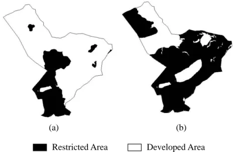
The Wu-Tu watershed is located east of the Taipei Basin in northern Taiwan. Area, mean elevation and mean slope of the watershed are approximately 204.41 km2, 242.00 m and 0.005°, respectively. Under an increasing population, the watershed has become intensively urbanized with an annual average population increase of approximately 2.70% during 1987–1997, especially in the down-stream area of the watershed (Lin et al., 2007). The recent average annual population growth rate has been approximately 1.05%, lower than that before 1997. For land use simulation, data are required for the land use distribution and a number of biophysical and socio-economic parameters considered as potential factors driving the land use pattern. This study obtained land use data in 1999 from the Soil and Water Conservation Bureau of Council of Agriculture, Taiwan. Land use maps, which were generated and digitized by the Soil and Water Conservation Bureau based on 1:5000 aerial photographs taken in 1999, distinguish among 33 land use types in a vector format. According to the definitions of land use types by the Construction and Planning Agency of the Ministry of Interior Taiwan, the land use types were converted into five types including agricultural land, forest, built up area, grassland, and water body. The proportions of agricultural land, forest, built up area, grassland, and water body in 1999 were 1%, 83%, 6%, 3% and 7%, respectively (Fig. 1).

(11)

Figure 1. Land uses of Wu-tu watershed in 1999.

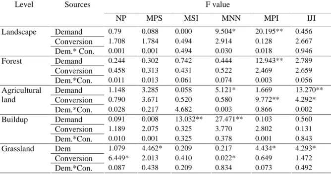
In this study, it was assumed that the driving factors of land use changes were demography, infrastructure, geomorphology and soil-related variables including altitude, slope, distance to river, soil erosion coefficient, soil drainage, distance to major road, distance to built up area, distance to urban planning area, and population density. To simulate the impact of climate change on different scenarios, we set four scenarios: Scenarios I (Low development demand and free Conversion), II (High development demand and free conversion), III (High development demand and agricultural protection conversion) and IV (Low development demand and agricultural protection conversion). Two land-use demands (namely low and high development demand), based on annual birth rates of 1.17% and 1.50%, are used as input data to further simulate land-use scenarios from 2000 to 2020. The 1995 agricultural land release policy of the Council of Agriculture, Executive Yuan, Taiwan, involves two land-use conversion rules (Free conversion and Agricultural protection conversion) based on the regulations and the agricultural land release policy. The free conversion specifies that agricultural, forest and grasslands can be converted into any of these three land uses, while built-up area and water bodies cannot be converted into other land uses. The agricultural protection conversion does not allow agricultural land to be converted into built-up area and forest (Fig. 2). To simulate different protection policies (free conversion and agricultural protection), there were four scenarios been set: Scenario A (Based on the baseline policy and the free conversion), Scenario B (Based on the conservation policy and the free conversion), Scenario C (Based on the baseline policy and the agricultural protection conversion) and Scenarios D (Based on the conservation policy and agricultural protection conversion). The first rule (Free Conversion) specifies that agricultural,

(12)

forest and grasslands can be converted into any of these three land uses, and built up area and water bodies cannot be converted into other land uses. The second rule (Agricultural protection) does not allow agricultural land to be converted into built up area and forest. These two rules allow us to compare the release and unreleased agricultural land policies.

(a) (b)

Figure 2. Spatial policies (a) the baseline policy (b) the conservation policy within the study watershed.

To simulate the scale effect, grain size in maps of land-use and driving factors were aggregated from 50 m to 75 m, 100 m, 125 m and 150 m resolutions. In this study, the conservation planning strategy, which included both an agricultural protection conversion and a large protected area, was simulated for the study area based on land-use demand and conversion rules with a land-use demand of an annual birth rate of 1.50%. This large protected area is overseen by a conservation plan that protects hillsides, water supply sources and large forested areas that are located primarily upstream in the watershed.

(2)Empirical land-use change model

The Conversion of Land Use and its Effects (CLUE-s) model comprises two parts: a non-spatial demand module; and, a spatially explicit allocation procedure. The non-spatial module calculates the area change for all land uses at the aggregate level (Verburg et al., 2002). In the spatial explicit allocation procedure, non-spatial demands are converted into land use changes at various locations in the study area. Yearly land use demands, which have to be defined prior to the allocation procedure, can be set by various approaches, such as economic models. The allocation procedure is based on a combination of empirical and spatial analyses and dynamic modeling

(13)

(Verburg et al., 2002). The model allocates land-use change by an iterative procedure utilizing probability maps and decision rules in combination with actual land-use maps and demand for different land-uses (Verburg et al., 2002). A preliminary allocation for iteration variables is given an equal value for all land-use types by allocating land-use types with high total probability of land-use for the considered grill cell. The value of the iteration variable is increased for land-use types for which the allocated area is smaller than the demand area. Iteration continues until the aggregated cover of all grid cells equals land-use demands.

Probability maps for all land-use types are calculated with logistic regression models. The relationships between land-uses and driving factors are then obtained using stepwise logistic regression as follows:



    m j ij j i i X P P Log 1 0 ) 1 (   (1)

where i is the i-th grid cell, P is the probability of a land-use type occurring in ai grid cell, j is the j-th driving factors, Xij is the driving factor, m is the number of

driving factors,  is the intercept of the regression model and0  is the coefficientj for each driving factor in the model. Relative operating characteristic (ROC) is applied to assess the goodness-of-fitofthemodel’slogisticregressions.TheROC value is defined as the area under the curve linking the relationship between the proportion of true positives versus the proportion of false positives for an infinite number of cut-off values (Overmars and Verburg, 2005). In this study, the forward stepwise logistic regression and ROC analyses were performed using the Statistical Package for the Social Sciences (SPSS) for Windows (SPSS Inc., Illinois, USA).

(3)Landscape metrics

To assess changes of land use patterns for the different land use scenarios, landscape metrics are calculated using FRAGSTATS in GIS software ArcView (McGarigal and Marks, 1995). In order to eliminate redundant information of land use patterns, seven landscape indices including Number of Patches (NP), Mean Patch Size (MPS), Total Edge (TE), Mean Shape Index (MSI), Mean Nearest Neighbor (MNN) and Interspersion and Juxtaposition Index (IJI), were used to present land use composition and configuration (size, edge, shape, isolation and interspersion of patches). Furthermore, to identify the effects of changing the grain size and area on spatial patterns of simulated land-use, landscape configuration metrics, including Number of Patches (NP), Mean Patch Size (MPS), Total Edge (TE) and Mean Shape Index (MSI), and landscape composition metrics, including Shannon’s Evenness

(14)

Index (SHEI) and Shannon’s Diversity Index (SHDI) at landscape level were calculated.

(4)Hydrological model

In the Generalized Watershed Loading Functions model, streamflow comprises surface runoff (Qt) calculated by Soil Conservation Service Curve Number and

groundwater discharge (Gt) estimated by modeling a shallow groundwater aquifer as a

linear reservoir. Storage of a shallow saturated zone is calculated by the following water balance equation (Tung, 2001):

t t t t t S PC G D S_1     (2) t t rS G  (3)

where St(cm) is the water content of a shallow ground water aquifer at the beginning

of day t, PCtis the percolation (cm) and Dtis the deep seepage (cm) during day t, r is

the recession coefficient. Percolation proceeds when soil moisture of an unsaturated zone exceeds field capacity, and is calculated by

] ,

0

max[ U I ET U*

PC_t  _t _t  _t  (4)

where Utis the soil moisture content of a root zone (cm) at the beginning of day t, It

is the infiltration (cm), ETt is the evapotranspiration (cm) during day t, and U*is the

maximum soil water capacity (cm). Infiltration can be calculated by t

t

t R Q

I   (5)

where Rt is rainfall. Evapotranspiration is affected by atmospheric conditions and

use and soil moisture content, whose relationship is described as follows (Tung, 2001): ] , [ st ct t t t t Min k k PET U I ET     (6)

where kst and kct are the coefficients of soil moisture stress and land cover,

respectively, and PETtis the potential evapotranspiration calculated with the Hamon

equation (Hamon, 1961; Tung, 2001). Water content in the unsaturated zone is traced by t t t t t U I ET PC U _1     (7)

where Ut+1(cm) and Ut (cm) are the moisture contents of the surface unsaturated soil

zone in excess of the field capacities on days t+1 and t, respectively, It (cm) denotes

the amount of water that infiltrates on day t, ETtrepresents the evapotranspiration (cm)

during day t, and PCt (cm) is the amount of percolation into the deep saturated zone

(15)

(5)Climate change scenarios

This study used rainfall and precipitation data from three GCMs (General circulation models) simulations, namely CGCM1, HadCM2 and GFDL-R15, representing three modeling centers, namely the Canadian Centre for Climate Modeling and Analysis, the Hadley Centre for Climate Prediction and Research, and the USA Geophysical Fluid Dynamics Laboratory. The future temperature change in the study area is assumed to be the same as the difference between the temperatures simulated using GCMs for the future and current conditions at the nearest grid point. Consequently, future climate scenarios can be estimated as follows (Tung et al., 2005)

) ( mT,Future mT,Current mT

mT   

   (8)

where  andmT denote current and future mean monthly temperature (°C)mT respectively, and mT ,Current, Current and mT ,Future, Future represent simulated mean monthly temperatures (°C) under the current and future climate conditions respectively. The change in precipitation is assumed to be the ratio of the precipitation for the future condition to that for the current condition (Tung et al., 2005):

) ( mP,Future mP,Current mP

mP   

    (9)

where  andmP  are current and future mean monthly precipitation (cm),mP respectively, while mP,Current ,Current and mP,Future ,Future are simulated mean monthly precipitation (cm) under the current and future climate conditions, respectively. The predictions of the GCM equilibrium experiments (1995 version) are downloaded from the US Country Studies Program, which is available on the web at the NCAR ftp site (ftp://ncardata.ucar.edu/pub).

3. Results

(1) Relationship between land-use and climate change A.Driving factors of land-use change

Table 1 lists the estimated coefficients and Relative Operating Characteristic values of the forward stepwise logistic regression models for all land uses (Lin et al., 2007). The fitted logistic models are used to calculate probabilities of occurrence for all land use types. The Relative Operating Characteristic values for the models range from 0.74 to 0.98, suggesting that the models are capable of explaining the spatial variation of land use patterns. Driving factors include altitude, distance to urban planning area, population density and the soil erosion coefficient, each of which contributes positively to explaining the spatial distribution of agricultural land in the

(16)

study area. Distance to major roads, slope and distance to built up areas have negative contributions on predicting the presence of agricultural land. Distance to river, elevation, slope, distance to built up area, and soil erosion contribute positively to the probability of forest in the study watershed. Additionally, factors distance to major roads and population density negatively impact the occurrence of forest. The logistic regression model for predicting built up area includes three negative coefficients of driving factors (slope, distance to built up area and soil erosion coefficient) and one minor positive factor (population density). Finally, the model for grassland has two positive factors (distance to major roads, soil drainage) and five negative factors (distance to river, elevation, slope, distance to built up area and distance to urban planning area).

Table 1. Logistics regression model for land use types.

Variable agriculture forest buildup grassland

Dtm 0.0015 0.0016 - -0.0043 Slope -0.041 0.0653 -0.0203 -0.0278 Popd 0.0002 -0.0001 3.17E-05 -Droad -0.0012 -0.0002 - 0.0011 Driver - 0.0001 - -0.0002 Dbuild -0.0019 0.0069 -0.0627 -0.0025 Dzone 0.0003 - - -9.34E-05 Odr - - - 0.467 Soilk 2.1461 4.6479 -1.8691 -Constant -3.1464 -1.4859 1.5537 -2.3934 ROC 0.735 0.88 0.983 0.757 a

Dtm: altitude; Slope: slope; Popd: population density; Droad: distance to major road; Driver: distance to river; Dbuild: distance to buildup area; Dzone: distance to urban planning area; Odr: soil drainage; Soilk: soil erosion coefficient.

b

-: not significant and not included in model at 0.05 significant level.

B.Statistical test for landscape metrics among land-use scenarios

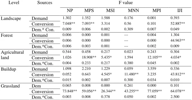
The two-way ANOVA results for all landscape metrics and four land-use scenarios at the landscape and class levels in the entire, upstream and downstream study watersheds are listed in Tables 2, 3 and 4, respectively. The ANOVA results for landscape metrics indicate that the landscape metrics Mean Nearest Neighbor and Mean Proximity Index of land-use scenarios at the landscape level in the study watershed differed significantly with demand during the simulation period for the entire watershed (Table 2). Patch Number, Mean Patch Size and Interspersion and

(17)

Juxtaposition Index for the land-use scenarios at the landscape level differed significantly with conversion policies during the simulation period in the upstream watershed (Table 3). At the landscape level, only Mean Nearest Neighbor differed significantly with demands and conversion policies during the simulation period in the downstream watershed (Table 4).

Table 2. Two-way ANOVA for the effects of land use demand and conversion on landscape metrics in the entire watershed.

F value

Level Sources

NP MPS MSI MNN MPI IJI

Demand 0.79 0.088 0.000 9.504* 20.195** 0.456 Conversion 1.708 1.784 0.494 2.914 0.128 2.667 Landscape Dem.* Con. 0.001 0.001 0.494 0.030 0.018 0.946 Demand 0.244 0.302 0.742 0.444 12.943** 2.789 Conversion 0.458 0.313 0.431 0.522 2.469 2.659 Forest Dem.*Con. 0.011 0.013 0.061 0.074 0.003 0.056 Demand 1.148 3.285 0.058 5.121* 1.669 13.270** Conversion 0.790 3.671 0.520 0.580 9.772** 4.292* Agricultural land Dem.*Con. 0.028 0.217 4.682 0.003 0.866 0.002 Demand 0.091 0.008 13.032** 27.471** 0.103 0.560 Conversion 1.189 2.075 0.325 3.770 2.802 0.131 Buildup Dem.*Con. 0.010 0.001 0.325 0.378 0.001 0.843 Dem 1.079 4.462* 0.209 0.217 4.434* 4.293* Conversion 6.449* 2.013 0.410 0.022* 0.649 1.472 Grassland Dem.*Con. 0.087 0.438 0.209 0.834 0.073 0.492 a

*: significant at 0.05.b**: significant at 0.01.cDem.: Demand.dCon.: Conversion.

At the agricultural land class level, landscape metrics Mean Nearest Neighbor and Interspersion and Juxtaposition Index of land-use scenarios varied significantly with demands during the simulation period for the entire watershed (Table 2). The Mean Proximity Index and the Interspersion and Juxtaposition Index of land-use scenarios at the agricultural land class level differed significantly with conversion policies during the simulation period (Table 2). At the built-up class level, the landscape metrics Mean Shape Index and Mean Nearest Neighbor of land-use scenarios differed significantly with demands throughout the simulation period. None of the landscape metrics for land-use scenarios at the built up class level differed significantly with conversion policies and the interaction of demands and conversion policies during the simulation period (Table 2). Mean Patch Size, Mean Proximity Index and Interspersion and Juxtaposition Index for land-use scenarios at the grassland class level differed significantly with demands during the simulation period. Moreover, Patch Number and Mean Nearest Neighbor for land-use scenarios at the grassland class level differed significantly with conversion policies during the

(18)

simulation period.

For the upstream watershed, landscape metrics Mean Patch Size, Mean Shape Index, Mean Proximity Index and Interspersion Juxtaposition Index of land-use scenarios only differed significantly with conversion policies during the simulation period at the agricultural land class level (Table 3).

Table 3. Two-way ANOVA for the effects of land use demand and conversion on landscape metrics for upstream watershed.

F value

Level Sources

Demand 1.302 1.352 1.588 0.176 0.001 0.393 Conversion 7.048** 7.093** 3.314 0.56 0.101 52.887** Landscape Dem.* Con. 0.009 0.006 0.002 0.309 0.007 0.049 Demand 0.006 0.000 0.001 --- 0.004 1.304 Conversion 0.006 0.000 0.000 --- 0.000 44.963** Forest Dem.*Con. 0.006 0.003 0.001 --- 0.002 0.009 Demand 0.544 0.458 0.217 0.023 0.243 0.304 Conversion 1.026 18.908** 5.435* 1.594 12.105** 4.034* Agricultural land Dem.*Con. 0.004 0.233 0.217 0.380 0.045 0.002 Demand 1.098 2.210 1.229 0.059 3.559 0.336 Conversion 0.052 0.643 4.545* 11.480** 3.235 43.812** Buildup Dem.*Con. 0.015 0.002 0.007 0.300 0.034 0.010 Dem 0.065 0.008 0.000 0.261 0.000 0.101 Conversion 73.848** 59.056** 26.344** 43.255** 77.059** 64.078** Grassland Dem.*Con. 0.003 0.008 0.378 0.050 0.002 2.500

Moreover, at the built up class level, Mean Shape Index, Mean Nearest Neighbor and Interspersion Juxtaposition Index of land-use scenarios differed significantly with conversion policies throughout the simulation period in the upstream watershed (Table 3). All landscape metrics for land-use scenarios at the grassland class level differed significantly with conversion policy during the simulation period in the upstream watershed (Table 3).

For the downstream watershed, the landscape metrics Mean Patch Size, Mean Proximity Index and Interspersion and Juxtaposition Index for land-use scenarios differed significantly with demand and conversion policies during the simulation period at the agricultural land class level (Table 4).

(19)

Table 4. Two-way ANOVA for the effects of land use demand and conversion on landscape metrics for downstream watershed.

F value

Level Sources

Demand 1.829 1.996 0.889 4.699* 1.581 2.968 Conversion 0.194 0.217 2.000 14.795** 2.133 0.043 Landscape Dem.* Con. 0.000 0.000 0.889 0.017 0.001 0.002 Demand 0.353 0.156 0.465 0.452 1.579 3.146 Conversion 0.186 0.628 0.633 0.411 4.054 0.026 Forest Dem.*Con. 0.007 0.937 0.070 0.064 0.015 0.050 Demand 0.949 4.147* 0.022 1.646 12.553** 5.535* Conversion 1.192 8.653** 1.075 2.977 5.281* 22.177** Agricultural land Dem.*Con. 0.055 0.461 4.934* 0.416 0.920 0.003 Demand 1.246 2.022 0.077 3.590 2.807 2.510 Conversion 0.345 0.109 2.764 8.208** 0.119 0.024 Buildup Dem.*Con. 0.043 0.011 0.691 0.244 0.000 0.046 Dem 5.330* 3.597 0.764 5.109* 0.823 1.631 Conversion 1.998 3.349 0.309 0.496 1.858 5.984* Grassland Dem.*Con. 0.085 0.807 0.006 0.106 0.071 0.470

The Mean Shape Index of land-use scenarios at the agricultural land class level differed significantly with the interaction of demand and conversion policies during the simulation period in the downstream watershed (Table 4). Moreover, at the built up class level, only Mean Nearest Neighbor of land-use scenarios differed significantly with conversion policies throughout the simulation period in the downstream watershed. None of the landscape metrics for land-use scenarios at the built-up class level differed significantly with conversion policies and the interaction of demands and conversion policies during the simulation period for the downstream area (Table 4). Patch Number and Mean Nearest Neighbor for land-use scenarios at the grassland class level differed significantly with demands during the simulation period. However, only Interspersion and juxtaposition Index for land-use scenarios at the grassland class level differed significantly with conversion policies during the simulation period for the downstream watershed (Table 4).

C.Hydrological components under land-use scenarios with no climate change

Based on historical weather data (i.e. data from a period with no climate change), streamflows, surface runoffs and groundwater discharges are simulated using the GWLF model and further land-use changes for the period 2000–2020 for both the upstream watershed and the entire watershed. To compare annual variations in hydrological components, the differences in the annual streamflow, annual surface runoff and annual groundwater discharge based the land uses in 1999 (no change) and

(20)

hydrological components (based on land-use demands and four land-use scenarios for the period 2000–2020) in the upstream watershed and the entire watershed during the simulation period, the annual streamflows, runoff and groundwater discharges are calculated based on simulated monthly streamflows (Figs. 3 and 4).

Differences in annual stream flow due to land-use change scenarios gradually increased to 0.16% (scenario I), 0.25% (scenario II), 0.25% (scenario III) and 0.25% (scenario IV) during the simulation period for the upstream area (Fig. 3(a)). Differences in annual surface runoff due to land-use change scenario increased to 1.11% (scenario I), 1.47% (scenario II), 1.47% (scenario III) and 1.44% (scenario IV) during the simulation period in the upstream area (Fig. 3(b)). Moreover, differences in annual groundwater discharge due to land-use change scenario decreased to 0.80% (scenario I), 0.98% (scenario II), 0.98% (scenario III) and 0.94% (scenario IV) during the simulation period in upstream area (Fig. 3(c)).

For the entire watershed, the differences in annual stream flows between land-use change and no change gradually increase to 0.60% and 0.50% for the high and low demands during the simulation period (Fig. 4(a)). Differences in annual surface runoff between no land-use change and land-use change scenarios increased to 4.00% (High demand) and 3.22% (Low demand) during the simulation period for the entire watershed (Fig. 4(b)). Furthermore, differences in annual groundwater discharge between no land-use change and land-use change situations decreased to 2.80% (Low demand) and 3.50% (High demand) during the simulation period (Fig. 4(c)) for the entire watershed.

(21)

Scenario I Scenario II Scenario III Scenario IV -0.04% 0.02% 0.08% 0.14% 0.20% 0.26% 2000 2005 2010 2015 2020 Year -0.20% 0.40% 1.00% 1.60% 2000 2005 2010 2015 2020 Year -1.00% -0.60% -0.20% 0.20% 2000 2005 2010 2015 2020 Year

Figure 3. Cumulative change of (a) streamflow, (b) runoff, (c) groundwater discharge in upstream watershed.

(a)

(b)

(22)

Low Demand High Demand 0.00% 0.10% 0.20% 0.30% 0.40% 0.50% 0.60% 0.70% 2000 2005 2010 2015 2020 Year 0.00% 1.00% 2.00% 3.00% 4.00% 5.00% 2000 2005 2010 2015 2020 Year -4.00% -3.50% -3.00% -2.50% -2.00% -1.50% -1.00% -0.50% 0.00% 2000 2005 2010 2015 2020 Year

Figure 4. Cumulative change of (a) streamflow, (b) runoff, (c) groundwater discharge in the entire watershed.

(a)

(c) (b)

(23)

D.Hydrological components under land-use scenarios and climate change

Based on climate scenarios of GCM models, streamflows, surface runoff and groundwater discharge is simulated using the GWLF model and simulated 2020 land-use for four land-use scenarios in the upstream watershed and land-use demands in the entire watershed. To compare annual variations in hydrological components, the differences in the annual streamflow, annual surface runoff and annual groundwater discharge based on the 1999 and 2020 land-use scenarios in the upstream watershed and the entire watershed the annual streamflows, runoff and groundwater discharges are calculated based on simulated monthly streamflows (Figs. 5 and 6). The differences in annual stream flow between the no land-use change situation and each scenario change decreased from 0.21% to 1.45% (for CGCM and GFDL) and increased from 1.31% to 1.43% (for HADCM) for the scenario for the year 2020 in the upstream area under climate change (Fig. 5). Differences in annual surface runoff between the no land-use change situation and each scenario increased from 2.51% to 6.19% for all land-use scenarios and all climate changes in the upstream area. Differences in annual groundwater discharge between the no land-use change situation and each scenario decreased from -3.12% to -6.68% for all land-use scenarios under all climate change scenarios (CGCM, GFDL and HADCM) in upstream area (Fig. 5).

(24)

-8% -4% 0% 4% 8% Rainf all GW _Runoff Strea mflow -8% -4% 0% 4% 8% Rainf all _GW Runo ff Strea mflow -8% -4% 0% 4% 8% Rainf all _GW Runo ff Strea mflow -8% -4% 0% 4% 8% Rainf all _GW Runo ff Strea mflow

Figure 5. Difference in simulated hydrological components between (a) Scenario I, (b) Scenario II, (c) Scenario III, (d) Scenario IV and no land use change under climate change in upstream watershed.

(a)

(d) (c)

(25)

The differences in annual stream flows between the land-use change and no change situations increased from 0.16% to 1.85% (CGCM and HADCM) and decreased from 0.86% to 0.94% for two land-use demands by 2020 in the entire watershed (Fig. 6). Differences in annual surface runoff between the land-use change and no change situations increased from 4.70% to 7.54% (Low demand) and 5.47% to 8.29% (High demand) in 2020 under the climate change scenario (Fig. 6). Differences in annual groundwater discharge between land-use change and no change decrease from -5.44% to -8.69% (Low demand) and from -6.20% to -9.42% (High demand) by the year 2020 in the climate change scenario (Fig. 6).

-10% -5% 0% 5% 10%

Rainfall GW Runoff Streamflow

-10% -5% 0% 5% 10%

Rainfall GW Runoff Streamflow

Figure 6. Difference in simulated hydrological components between (a) low demand, (b) high demand and no land use change under climate change in the entire watershed.

(2) Influence of land-use policy on hydrology and landscape patterns A.Landscape metrics

The change proportions of each land use type between 1990 and 2020 for agricultural land, forest, built up area and grassland was -0.36%, -1.77%, 2.37%, and 0.24%. The results of the land use model were used to calculate various landscape metrics. All landscape metrics display similar values for scenarios A and C (The baseline policy) as well as for scenarios B and D (The conservation policy). Figure 6 shows the values of the other landscape metrics at the landscape level. The values of Patch Number, Total Edge, and Interspersion and Juxtaposition Index decreased from 2000 to 2020 for all scenarios (Figs. 7(a), (c) and (f)). Figures 7(b) and (e) show that the values of Mean Patch Size and Mean Nearest Neighbor of all land use scenarios increased during the period 2000–2020. The values of Patch Number, and Interspersion and Juxtaposition Index of land use scenarios A and C (The baseline

(b) (a)

(26)

Scenario A Scenario B _{Scenario C} Scenario D

policy) are greater than those for scenarios B and D (The conservation policy) (Figs. 7(a) and (f)).

(a) (b)

(c) (d)

(e) (f)

Figure 7. Landscape metrics of land use scenarios at landscape level (a) Number of Patches, (b) Mean Patch Size, (c) Total Edge, (d) Mean Shape Index, (e) Mean Nearest Neighbor, (f) Interspersion and Juxtaposition Index of land use scenarios at landscape level. 1.24 1.25 1.26 1.27 1.28 2000 2004 2008 2012 2016 2020 Year M e a n S h a p e In d e x 8.50 9.00 9.50 10.00 2000 2004 2008 2012 2016 2020 Year M e a n P a tc h S iz e (h a ) 1850 1900 1950 2000 2050 2100 2150 2200 2000 2004 2008 2012 2016 2020 Year N u m b e r o f P at c h e s 1.02E+06 1.03E+06 1.03E+06 1.04E+06 1.04E+06 1.05E+06 2000 2004 2008 2012 2016 2020 Year T o ta l E d g e (m ) 115 117 119 121 123 125 2000 2004 2008 2012 2016 2020 Year M e a n N e a re st N e ig h b o r D is ta n c e (m ) 78 79 80 81 82 83 84 2000 2004 2008 2012 2016 2020 Year In te rs p e rs io n a n d Ju x ta p o si ti o n In d e x (% )

(27)

Moreover, the values of Mean Patch Size and Mean Nearest Neighbor for scenarios B and D (The conservation policy) are larger than those for scenarios A and C (The baseline policy) (Figs. 7(b) and (e)). Finally, the values of Total Edge in scenarios B and D (The conservation policy) are greater than those in scenarios A and C (The baseline policy) in 2000–2006 and less than those in scenarios A and C during 2006–2020. The Mean Shape Index values for all land use scenarios remained almost constant in 2000–2020, particularly for scenario B (Fig. 7(d)).

B.Stream flow under land use change demands

Ten-year (1993–2002) streamflow data were used to validate the simulated streamflow modeled by the Generalized Watershed Loading Function using historical weather data and parameters that include the recession coefficient, evapotranspiration coefficient and the Curve Number for the study watershed. Figure 8 shows the monthly observed streamflow versus the simulated monthly streamflow, and the mean measured monthly streamflow versus the mean predicted monthly streamflows.

The R2 value of the linear regression model for the monthly observed streamflows and simulated streamflows during the ten-year period is 0.79. Moreover, the R2 value of the linear regression model of the monthly mean observed streamflows and the mean simulated streamflows during the ten-year period is almost 1.0. Both linear regression models are significant at a 0.01 significance level.

Based on historical weather data, hydrological components are simulated using the Generalized Watershed Loading Function model with the above parameters (the recession coefficient, evapotranspiration coefficient and the Curve Number) and future land use changes from 2000–2020. The differences in the annual streamflow, surface runoff and groundwater discharge between 1999 and the simulation period (2000-2020) are calculated from simulated monthly streamflows (Fig. 9). The differences in annual streamflow due to land use change gradually increase to 0.61% during the simulation period. Moreover, differences in annual surface runoff between the land use change and no change increase by 4.00% during the simulation period. Finally, differences in annual groundwater discharge decrease by 3.50% during the simulation period.

(28)

Observed Simulated

Figure 8. (a) Monthly observed streamflow vs. simulated monthly streamflow, (b) mean monthly observed streamflow vs. mean simulated monthly streamflow.

(a)

(29)

(a)

(b)

(c)

Figure 9. Difference in annual (a) streamflow, (b) run off, (c) groundwater discharge between land use in 1999 and land use in each simulated year.

(30)

(3) Scale effect on land-use change, landscape patterns and hydrological components A.Land-use change models in various grain sizes

The fitted logistic models were applied to predict probabilities for all land-use types and to measure the relationships between probabilities and driving factors for various resolutions. The ROC values for the models are 0.74–0.98, 0.73–0.97, 0.74–1.00, 0.75–1.00 and 0.76–1.00 for grain sizes of 50 m × 50 m, 75 m × 75 m, 100 m × 100 m, 125 m × 125 m, and 150 m × 150 m, respectively. Driving factors including elevation, population density and the soil erosion coefficient did not contribute to the logistic regression model for predicting agricultural land when the grain size was >100 m × 100 m. Distance from main roads and urban planning areas were not used in the regression model for calculating the probability of agricultural land at a grain size of 125 m × 125 m. Furthermore, the coefficients of population density in regression models became negative for the probability of agricultural land when the grain size was increased from 50 m × 50 m to large sizes. For predicting forested areas, distances from roads, distances from the river and distances from urban planning areas did not contribute to the logistic regression model when the grain size was >125 m × 125 m. The number of driving factors declined from 4 to 1 (distance from built-up areas) in the logistic regression model for predicting built-up when the grain size was >100 m × 100 m. Furthermore, soil drainage, distances from urban planning areas and distances from rivers did not contribute to logistic regression models for predicting grassland at grain sizes of 75 m × 75 m, 100 m × 100 m, and 150 m × 150 m.

B.Simulated land-use patterns for changing scales

The landscape metrics in the landscape level results show that increasing grain size from 50 m × 50 m to 150 m × 150 m decreased the values of NP, TE and MSI for simulated land-uses during the simulated period in both the upstream watershed and the entire watershed (Figs. 10(a), (c), (d), and 11(a), (c), (d)). Conversely, the values of MPS increased in both the upstream watershed and the entire watershed at the landscape level when grain size was increased during the simulated period (Figs. 10(b) and 11(b)). Values of SHDI and SHEI tended to stair-step upward with similar magnitudes during the simulated period when grain size increased from 50 m50 m to 125 m 125 m for the upstream watershed (Figs. 10(e) and (f)). Values of SHDI and SHEI tended to stair-step upward with similar magnitudes during the simulated period when grain size increased from 50 m × 50 m to 150 m × 150 m for the entire watershed (Figs. 11(e) and (f)).

(31)

Figure 10. Landscape metrics at landscape level for the upstream watershed (A) Number of Patch, (B) Mean Patch Size, (C) Total Edge, (D)Mean Shape Index , (E) Shannon’s Diversity Index, (F) Shannon’s Evenness Index.

(32)

Figure 11. Landscape metrics at landscape level for the entire watershed (A) Number of Patch, (B) Mean Patch Size, (C) Total Edge, (D)Mean Shape Index , (E) Shannon’s Diversity Index, (F) Shannon’s Evenness Index.

(33)

C.Simulated hydrological components for changing scales

Simulated groundwater discharge decreased when grain sizes in land-use simulations increased from 50 m × 50 m to 100 m × 100 m, and groundwater discharge increased when grain sizes in simulated land-use increased from 125 m × 125 m to 150 m × 150 m (Fig. 12(a)). Conversely, the simulated surface runoff increased when grain sizes in land-use simulations increased from 50 m × 50 m to 100 m × 100 m, and declined when grain sizes for simulating land-use increased from 125 m × 125 m to 150 m × 150 m in the land-use planning strategy (Fig. 12(b)). Furthermore, both simulated groundwater discharge and surface runoff at various grain sizes during the simulated period had similar tendencies (increase and decrease) and magnitudes. However, the simulated streamflow for each grain size gradually increased from simulated year 2000, and tended to increase steadily in subsequent simulated years (Fig. 12(c)). The magnitudes of simulated streamflows at each grain size differed significantly in the upstream watershed, particularly the simulated streamflows for all land-use scenarios at grain sizes of 50 m × 50 m and 100 m × 100 m. Furthermore, the simulated streamflows in fine grain size increased more rapidly and had a tendency to remain stable earlier than those in other grain sizes, except those in a grain size of 100 m× 100 m (Fig. 12(c)).

(34)

Figure 12. Cumulative changes of (A) groundwater discharge, (B) surface runoff, (C) streamflow in the upstream watershed.

(35)

4. Discussion

(1)Responses of land-use and climate scenarios on hydrology

Spatial models, such as an explicit model forecasting land use, can help planners to evaluate long-term effects of development patterns on landscape structures and the value derived from such development (Wear and Bolstad, 1998; Turner et al., 2001). Improving our understanding of the complex relationships between the land and water is an important goal of both basic and applied research in landscape ecology (Turner et al. 2001). If only land-use changes were considered, then future land-use change scenarios had various impacts on the hydrological components (streamflow, surface runoff and groundwater discharge) through time and under various levels of land-use change pressure (various land-use demands). For upstream areas, the impacts on annual streamflow, surface runoff and groundwater discharge of scenario IV were 1.50, 1.30 and 1.17 times greater than those of scenario I. Moreover, various land-use demands and policies influenced future hydrological components in the study watershed, especially in highly developed areas. The influence on hydrological components in the study watershed increased with demand from built-up areas. For the entire watershed, the impacts on annual streamflow, surface runoff and groundwater discharge of the high development demand were 1.20, 1.24 and 1.25 times greater than those from the low development demand. Furthermore, the highest impacts on annual streamflow, surface runoff and groundwater discharge for the entire watershed were 1.50, 2.70 and 3.70 times higher than those for the upstream area. However, surface runoff from urban areas increased and groundwater discharge decreased as replacement of vegetation through development reduces infiltration.

Comparing the impacts of both land-use and climate changes on hydrology, climate changes impacted the hydrological components much more strongly than land-use changes for all scenarios in the study area, and had a particularly large impact on runoffs and groundwater discharges. However, the increases in precipitation caused by climate change increased annual surface runoff (1.37 to 2.32 times) more than did the no climate change situation for all land-use change scenarios in all climate change scenarios for the entire watershed in 2020. The impacts of climate changes on annual groundwater discharges were greater (1.71 to 1.96 times) than those of no climate changes during 2020 for the study watershed in all land-use scenarios. The impacts of climate changes on annual streamflow were slightly greater or less than those of no climate changes in 2020 for the study watershed for all land-use scenarios. These slight and varied differences may be due to the water balances of high changes (increases) of surface runoff and groundwater discharges (decreases) for all land-use scenarios in the study watershed.

(36)

Comparing the increase in the ratios of annual surface runoff between the upstream and entire area, the highest increase in the ratios of annual surface runoffs for the entire watershed were higher (1.35 to 1.87 times) than those in the upstream area for climate changes in 2020. Comparing the decreasing ratios of annual groundwater discharges in both the upstream and the entire areas, the highest decrease ratio of annual groundwater discharges in the entire watershed were higher (1.42 to 1.84 times) than in the upstream area in the climate change situation in 2020. The low change in streamflow could be explained by the water balance of increasing surface runoff and decreasing groundwater discharge in 2020. However, the impacts by considering both land-use and climate changes were significantly higher than by only considering climate change or land-use change for surface runoff and groundwater discharge. This study did not consider the interactions between land-use change and climate changes. For example, long-term directional changes in due to global warming or glacial cycles would eventually move a landscape out of present bounds (Turner et al. 2001). This issue should be also included in further related works.

(2)Driving factors

In this study, logistic models are estimated to explain the spatial variation in occurrence of the different land use types. The logistic model results for all land uses indicate that agricultural land locations are jointly determined by biophysical parameters (altitude, slope and soil erosion coefficients) and socio-economic characteristics, such as distance to major roads, distance to built up areas, distance to urban planning areas and population density. These analytical results showed that agricultural activity is complex and affected by both physical and socio-economic characteristics in the subject watershed, particularly by slope and soil conditions. The location and distribution of forests are influenced by all biophysical and socio-economic factors except distance to urban planning areas and soil drainage. This regression analysis showed that forest distribution is influenced by human activity and natural conditions in the watershed, especially the negative impact of road construction and urban sprawl resulting from population growth. However, the regression results confirm that each location possesses specific soil characteristics that influence the potential for natural and agricultural vegetation (Verburg et al., 2004) and its slope. The locations of built up areas are constrained by three socio-economic parameters and the soil erosion coefficient. The slope and distance to built up area have negative coefficients, implying that population pressure caused the expansion of built up areas into non-urban planning areas with low elevations. The locations of grasslands are influenced by all factors, except population density and the soil erosion coefficient. Only soil drainage and distance to road had positive coefficients in the

(37)

logistic model for grassland. This regression result indicates that grassland distributions, including natural succession and human-made development (e.g., parks and open spaces) are controlled by natural conditions (soil drainage and slope) and human activity. The distributions of most land use types are affected by socio-economic factors, implying that urbanization influences land use in the study watershed. The logistic regression results also confirm that the biophysical characteristics determine the potential benefits that can be achieved by allocating a particular land use at a certain locations (Verburg et al., 2004), and that different factors are required to capture the different processes resulting in specific land use patterns (Lambin, 1994; Serneels and Lambin, 2001). In this study, the Relative Operating Characteristic values vary between 0.74–0.98 depending on land use type, implying that the logistic regression model effectively explains land use distribution.

The effect of changes of scale on simulation results is often hard to detect (Farina, 2000). As scale changes, new patterns and processes may emerge, and controlling factors may shift even for the same phenomena (Wu and Li, 2006). For example, the relationship between land-use patterns and processes may be easy to identify at fine scales, where land-use change can be associated explicitly with activity of agents in a landscape (Jantz and Goetz, 2005). Observations made at fine scales may miss important patterns and processes operating on broader scales (Wu and Li, 2006). Conversely, broad-scale observations may not have enough detail to understand the fine-scale dynamics (Wu and Li, 2006). Land-use drivers that best describe land-use patterns quantitatively are often selected through logistic regression analysis (Overmars et al. 2003). However, fine-scale data for study watersheds may not always be available. In this study, the logistic regression results revealed that most land-uses were affected by socio-economic factors, suggesting that urbanization affects land-uses in the study watershed. Logistic regression indicated that biophysical features were incorporated as potential benefits that are experienced via a particular land-use at a certain location (Verburg and Veldkamp, 2004), and that different model factors are therefore required for different processes resulting in alteration of land-use (Lambin, 1994; Serneels and Lambin, 2001).

Changing resolution significantly influences variable composition and the regression coefficients for land-use regression models (de Koning et al., 1998; Verburg et al., 1999). Conversely, Kok and Veldkamp (2001) concluded that, although explanatory power increases, coarsening of spatial resolution does not influence the composition of the set of land-use determining factors significantly. Increased spatial resolution has been shown to both increase and decrease model performance (Ciret and Henderson-Sellers, 1989). In this study, the ROC values in simulating all land-uses in various grain sizes were >0.73 and were very similar for each land-use

(38)

type, implying that land-uses can be explained reasonably by the logistic regression models with their driving factors when grain size was changed in study cases. However, changing grain size did not influence prediction performance of regression models for all land-uses significantly, but there were significant changes to the composition of variables and the regression coefficients for land-use logistic regression models when the grain size was more than twice the finest grain size, particularly for built-up areas. Logistic regression revealed that altering grain size had various impacts on composition variables in regression models for various land-uses with spatial characteristics, such as the configuration and composition of land-uses. For instance, the built-up area was heterogeneous when using the finest grain size and was homogeneous when grain size was increased.

(3)Responses on land-use patterns

In urban and urbanizing areas, land cover change significantly influences the structure, function, and dynamics of ecological systems (Luck and Wu 2002). Potential future patterns of landscape structure can be examined by projecting the land-use pattern (Jenerette and Wu, 2001). In this study, land-use change model (CLUE-s), landscape metrics and ANOVA can effectively model and assess demand and conversion policies regarding future land-use patterns. Demand and conversion policies only significantly impacted the isolations of the future landscape patterns of the entire and downstream watershed at the landscape level during the simulation period. Conversion policies obviously impacted patch size and dispersion of future land-use patterns in the upstream watershed during the simulation period. At the landscape level, the conversion policies did not significantly impact the scenario land-use patterns for the entire watershed and downstream watershed, but did impact future land-use patterns of the upstream watershed during the simulation period. These minor impacts may result from land-use suitability, the minor change in land-use demand during 2000–2020, and the pre-urbanized pattern influencing further simulation of land-use at the landscape level for the entire study area and the downstream watershed. Furthermore, the landscape matrix (forest) and its changes also influenced land-use patterns in various land-use scenarios at the watershed landscape level, especially in upstream areas.

Landscape metrics provide an effective means of evaluating and comparing before and after conditions in a landscape plan for a particular landscape (Gustafson, 1998; Leitao and Ahern, 2002; Corry and Nassauer, 2005). At the landscape level, patterns of all land use scenarios have similar tendencies and different magnitudes under different spatial policies during the simulation period. The land use patterns in the baseline policy scenarios involve smaller but more closely positioned patches

(39)

compared to the scenarios with the conservation policy. Moreover, the land use patterns in conservation policy scenarios are more isolated than those in baseline policy scenarios. The patterns in the land use change area with the baseline policy are more fragmented than those with the conservation policy at the landscape level. No association was found between conversion policies and land use patterns, but different spatial policies resulted in significantly different landscape metrics at the landscape level. Interaction of the conversion and spatial policies at the landscape level only resulted in significant differences in patch. These relatively minor effects may result from the relatively small change in land use demand during 2000–2020, and the influence of initial land use patterns on future land use.

Information may be available at a variety of scales and it may be necessary to extrapolate information from one scale to another (Leitão et al., 2006). Spatial models, such as an explicit model forecasting land-use, can help planners to examine the long-term effects of development patterns on landscape structures and the values derived from such development (Wear and Bolstad 1998; Turner et al., 2001). The scale at which land-use data are represented can influence quantification of land-use patternsand amodel’sability to replicate spatialpatterns(Jeneretteand Wu,2001; Jantz and Goetz, 2005). Landscape metrics are effective tools for assessing and comparing before and after conditions in a landscape plan (Gustafson, 1998; Leitão and Ahern, 2002; Corry and Nassauer, 2005; Leitão et al., 2006; Lin et al., 2007). The metrics are useful also for assessing scale effects on land-use patterns. For instance, Turner et al. (1989) reported that the diversity index decreased linearly with increasing logarithm grain size. Wu (2004) reported that as area increased, MPS was changed by much less than in the case of changing grain size. In this study, NP, MPS, TE and MSI responded consistently to changes of grain size in each simulated year. SHDI and SHEI presented stair-step responses with changing simulated year when grain size changed. The stair-step responses are similar to the results reported by Turner et al. (1989) and Wu (2004), which confirmed that the apparent proportion of the landscape in different cover types changes with grain size (Turner et. al, 1989). Moreover, the spatial arrangement of the land cover also influences the rate at which land cover types disappear (Turner et al., 1989).

In this study, annual mean values of NP, TE and MSI consistently exhibited a power relation with grain size during the simulated period in both the upstream and the entire area of the watershed. Annual mean values of MPS exhibited a linear relation with grain size in both the entire and the upstream area of the watershed. The landscape metrics-scaling relations results during the simulated period (multiple time-scale) in the study area presented a metrics-scaling relation similar to the results presented by Wu (2004). Annual mean values of SHDI and SHEI exhibited