以區域最佳解為基礎求解流程式排程問題的新啟發式方法 - 政大學術集成

全文

(1)國立政治大學資訊管理學系. 博士學位論文指導教授:陳春龍博士、陳俊龍博士. 立. 政治大. ‧ 國. 學. 以區域最佳解為基礎求解流程式排程問題的新啟發式方法. ‧. sit. y. Nat. A new heuristic based on local best solution. n. er. io. for Permutation Flow Shop Scheduling al v i n Ch engchi U. 研究生：曾宇瑞中華民國一百零一年七月.

(2) 摘要本研究開發一個以區域最佳解為基礎的群體式 (population-based) 啟發式演算法(簡稱 HLBS)，來求解流程式排程（flow shop）之最大流程時間的最小化問題。其中，HLBS 會先建置一個跟隨模型來導引搜尋機制，然後，運用過濾策略來預防重複搜尋相同解空間而陷入區域最佳解的困境；但搜尋仍有可能會陷入區域最佳解，這時，HLBS 則會啟動跳脫策略來協助跳出區域最佳解，以進入新的區域之搜尋；為驗證 HLBS 演算法的績效，本研究利用著名的 Taillard 測試題庫. 政治大證明 HLBS 較其他知名群體式啟發式演算法(如基因演算法、蟻群演算法以及粒立. 來進行評估，除證明跟隨模型、過濾策略和跳脫策略的效用外，也提出實驗結果. ‧ 國. 學. 子群最佳化演算法)之效能為優。關鍵字：流程式排程，最大流程時間，啟發式方法. ‧. n. er. io. sit. y. Nat. al. Ch. engchi. i n U. v.

(3) Abstract This research proposes population-based metaheuristic based on the local best solution (HLBS) for the permutation flow shop scheduling problem (PFSP-makespan). The proposed metaheuristic operates through three mechanisms: (i) it introduces a new method to produce a trace-model for guiding the search, (ii) it applies a new filter strategy to filter the solution regions that have been reviewed and guides the search to new solution regions in order to keep the search from trapping into local optima, and. 政治大 become trapped at a local立 optimum. Computational experiments on the well-known (iii) it initiates a new jump strategy to help the search escape if the search does. ‧ 國. 學. Taillard's benchmark data sets will be performed to evaluate the effects of the trace-model generating rule, the filter strategy, and the jump strategy on the. ‧. performance of HLBS, and to compare the performance of HLBS with all the. sit. y. Nat. promising population-based metaheuristics related to Genetic Algorithms (GA), Ant. al. er. io. Colony Optimization (ACO) and Particle Swarm Optimization (PSO).. n. v i n C hScheduling, Makespan, Keywords: Permutation Flow Shop e n g c h i U Metaheuristic.

(4) 謝辭. 本論文得以順利完成，首先特別要感謝兩位恩師陳春龍博士與陳俊龍博士的包容與付出，兩年來不論課業或生活上遇到何種困境與挫折，您們總是亦師亦友的傾聽與協助，常讓我在沮喪之餘，能重燃信心；在論文進行期間您們更是不辭辛勞帶領我一點一滴累積相關知識，適時導正研究方向，並給予相當的支持與協助，使我遭遇的問題均能迎刃而解，獲益良多。其次要感謝口試委員林我聰博士、季延平博士和吳忠敏博士在百忙之中仍抽. 政治大. 空審閱論文，並給予許多寶貴的建議與指正，遂使本論文能夠更加充實與完備。. 立. 隨著博士班生涯接近尾聲，回想過去的酸甜苦辣，內心感觸良多，除還要感. ‧ 國. 學. 謝一路相挺的長官、同窗與家人外，也感恩有貴人季延平老師的諄諄善誘；最後要感謝的是我一生的摯愛燕君，為了讓我專心於課業，她主動分擔家庭重責，. ‧. 尤其每當熬夜寫程式時，她總是噓寒問暖，關懷之情溢於言表，讓我備感溫馨。. y. Nat. n. er. io. al. sit. 在此向您們獻上我最誠摯的謝意. Ch. engchi. i n U. v. 曾宇瑞謹誌.

(5) TABLE OF CONTENTS Chapter 1. Introduction ....................................................................................... 1 Chapter 2. Literature review ............................................................................... 3 2.1. Problem statement: PFSP-makespan ................................................ 3. 2.2. Genetic Algorithms (GA) .................................................................. 4. 2.3. Ant Colony Optimization (ACO) ...................................................... 6. 2.4. Particle Swarm Optimization (PSO) ................................................. 7. 政治大. Chapter 3. The proposed metaheuristic (HLBS) ................................................11. 立. Trace-model generating rule and solution construction method ......12. 3.2. Filter strategy ...................................................................................16. 3.3. Jump strategy ..................................................................................18. ‧. ‧ 國. 學. 3.1. Chapter 4. Computational experiments of HLBS ...............................................20. y. Nat. 4.2. Computational experiments of A-HLBS ..........................................28. n. al. er. sit. Computational experiments of B-HLBS...........................................20. io. 4.1. i n U. v. Chapter 5. Conclusions and further research .....................................................35. Ch. engchi. References .........................................................................................................37.

(6) LIST OF TABLES Table 3.1.1 The example for illustrating the trace-model generating rule and the solution construction method ................................................................................. 14 Table 4.1.1 Experimental factors.................................................................................. 21 Table 4.1.2 ANOVA table for testing the significance of the three factors .................. 23 Table 4.1.3 Results of Duncan’s test for different filter sizes ....................................... 23 Table 4.1.4 Results of Duncan’s test for different jump-rates...................................... 23. 政治大. Table 4.1.5 Computational Results of M-MMAS, PACO and B-HLBS (t30*) ................. 25. 立. Table 4.1.6 Computational Results of M-MMAS, PACO and B-HLBS (t60*) ................. 25. ‧ 國. 學. Table 4.1.7 Computational Results of M-MMAS, PACO and B-HLBS (t90*) ................. 26 Table 4.1.8 Results of the Paired Samples T-Test for M-MMAS, PACO and B-HLBS. ‧. under different computation times ......................................................................... 26. y. Nat. sit. Table 4.1.9 Computational Results of PSOvns, NEGAvns and B-HLBS ......................... 27. n. al. er. io. Table 4.2.1 Experimental factors.................................................................................. 28. i n U. v. Table 4.2.2 ANOVA table for testing the significance of the five factors ..................... 29. Ch. engchi. Table 4.2.3 Results of Duncan’s test for the five major factors.................................... 30 Table 4.2.4 Computational Results of HGA_RMA, B-HLBS and A-HLBS (t30*) ............ 32 Table 4.2.5 Computational Results of HGA_RMA, B-HLBS and A-HLBS (t60*) ............ 32 Table 4.2.6 Computational Results of HGA_RMA, B-HLBS and A-HLBS (t90*) ............ 33 Table 4.2.7 Results of the Paired Samples T-Test for HGA_RMA, B-HLBS and............. 33 Table 4.2.8 Computational Results of HGA_RMA, NEGAvns, PSOvns, B-HLBS and A-HLBS (t=n×m/10 seconds) .................................................................................... 34 Table 4.2.9 Results of the Paired Samples T-Test for NEGAvns, PSOvns, B-HLBS and A-HLBS (t=n×m/10 seconds) .................................................................................... 34.

(7) LIST OF FIGURES Figure 2.2.1 The pseudo-code for the general GA algorithm ........................................ 5 Figure 2.3.1 Pseudo-code for the general ACO algorithm ............................................. 7 Figure 2.4.1 Pseudo-code for the general DPSO algorithm with local search ............... 9. 立. 政治大. ‧. ‧ 國. 學. n. er. io. sit. y. Nat. al. Ch. engchi. i n U. v.

(8) Chapter 1. Introduction This research proposes a population-based metaheuristic based on the local best solution (HLBS) for the permutation flow shop Scheduling (PFSP-makespan). The candidate problem determines the best sequence of n jobs that are to be processed on m machines in the same order in order to minimize the complete time of the last job on the last machine (makespan). It has proved to be one of the most studied NP-hard scheduling problems in the strong sense (Garey et al. 1976) and has not been completely solved by exact algorithms. Therefore, the development of metaheuristics. 政治大 attention of many researchers 立in recent decades. These include genetic algorithm (GA) that find near-optimal solutions in a reasonable computational time has held the. ‧ 國. 學. (Chen et al., 1995; Reeves & Yamada, 1998; Ruiz et al., 2006; Chen et al., 2011), ant colony optimization (ACO) (Stützle, 1998a; Rajendran & Ziegler 2004; Ying & Liao,. ‧. 2004), particle swarm optimization (PSO) (Tasgetiren et al. 2004; Rameshkumar et al.. sit. y. Nat. 2005; Lian et al., 2006; Liao et al., 2007; Kuo et al., 2009; Zhang et al., 2010),. n. al. er. io. differential evolution (DE) (Andreas & Omirou, 2006; Onwubolu & Davendra, 2006;. i n U. v. Pan et al., 2008b), iterated greedy algorithm (IG) (Ruiz & Stützle, 2007), iterated. Ch. engchi. local search (ILS) (Stützle, 1998b), simulated annealing (SA) (Osman & Potts, 1989; Ogbu & Smith, 1990; Lin & Ying, 2011), tabu search (TS) (Widmer & Hertz, 1989; Reeves, 1993; Nowicki & Smutnicki, 1996; Watson et al., 2002; Grabowski & Wodecki, 2004) and hybrid metaheuristics (Zobolas et al., 2009; Liu & Liu, 2011). Several research papers reviewing heuristics for the candidate problem can be found in Framinan et al. (2004), Hejazi & Saghafian (2005), and Ruiz & Maroto (2005). The major idea of the proposed metaheuristic (HLBS) is that we think the local best solution in an iteration possesses important information about the solution regions searched, so the trace-model generated based on the local best solution should 1.

(9) provide valuable information for guiding the search to promising solution regions. In addition, we develop a new filter strategy to keep the search from trapping into local optimums and a new jumping strategy to help the search escape if it does trap into a local optimum. Computational experiments on the well-known Taillard's benchmark data sets (Taillard 1993) will be performed to evaluate the effects of the trace-model generating rule, the filter strategy, and the jump strategy on the performance of HLBS, and compare the performance of HLBS with other population-based metaheuristics such as Genetic Algorithms (GA), Ant Colony Optimization (ACO) and Particle. 政治大 thoroughly study the impact of the aforementioned strategies on the explorative 立 Swarm Optimization (PSO). A couple of new ideas will be further applied to. capability and the exploitative capability of the proposed algorithm in order to. ‧ 國. 學. improve its performance for solving PFSP-makespan.. ‧. The remainder of this research is organized as follows: Chapter 2 gives the. sit. y. Nat. literature review, the proposed algorithm HLBS is described in Chapter 3. Chapter 4. io. er. provides computational experiments, and conclusions and further research of this study are summarized in Chapter 5.. n. al. Ch. engchi. 2. i n U. v.

(10) Chapter 2. Literature review This research proposes a population-based metaheuristic for PFSP-makespan. Population-based metaheuristics share many common concepts of Evolutionary Algorithms (EA) which is a class of stochastic search and optimization techniques based on the principles of natural evolution. The basic process of population-based metaheuristics starts with a population of alternative solutions for a given problem in the initial generation. Then, the evolution operations of selection, replication and variation are applied to solutions chosen from the population to generate new. 政治大 survival concept of genetic 立evolution. Therefore, the solutions can be improved solutions for the next generation. The idea of the evolution operations is based on the. ‧ 國. 學. generation to generation until a termination criterion is satisfied. Most of the population-based metaheuristics are nature-inspired algorithms. In the following. ‧. sections, we will present the problem statement of PFSP-makespan and the literature. sit. y. Nat. review for three prominent population-based algorithms for PFSF-makepspan:. al. n. Optimization (PSO).. er. io. Genetic Algorithms (GA), Ant Colony Optimization (ACO) and Particle Swarm. Ch. engchi. i n U. v. 2.1 Problem statement: PFSP-makespan PFSP-makespan can be denoted as Fm||Cmax by Graham et al. (1979), where Fm represents a flow shop environment of m machines and Cmax refers to the makespan. We use the notation proposed by Graham et al. (1979); given a set J of n jobs, a set M of m machines and processing times pij for each job j on each machine i, the problem consists of scheduling all n jobs at each one of the m machines. The processing sequence of the jobs must be the same on all the machines and each job j can only start its execution on a machine i if both the previous job on the same machine i and the same job j on the previous machine i -1 have already been processed. Furthermore, 3.

(11) the order in which a job must pass through the machines is predefined and identical for all the jobs. The objective of this problem is to determine a job ordering that minimizes the completion time of the last job in the last machine, called the makespan. Although Garey et al. (1976) showed that the problem with two-machine can be solved in polynomial time, the general case with m machines is known to be NP-hard. Given a permutation schedule j1, . . . , jn for an m-machine flow shop, the completion time of job jk at machine i , Ci , j k , can be computed easily through a set of recursive equations: i. Ci , j1 = ∑ pl , j1. 立. l =1. 政治大 i=1, 2,…,m. (1). k=1, 2,…,n i=2,…,m; k=2,…,n. (3). er. io. sit. Nat. Then makespan, Cmax, is obtained by Cmax = Cm , j n. ‧. Ci , j k = max(Ci −1, j k , Ci , j k −1 ) + pi , j k. (2). y. l =1. 學. C1, j k = ∑ p1, jl. ‧ 國. k. al. v i n Genetic Algorithms (GA),C developed by John Holland h e n g c h i U in the 1970’s, are search n. 2.2 Genetic Algorithms (GA). algorithms that are based on the idea of genetic evolution. Genetic evolution implies that the optimum parents survive and generate better offspring. The same concept underlies the development of Genetic Algorithms (GA). In order to apply GA to a problem, generally the solution space of the problem is represented by a population of structures where each structure is a possible solution to the problem. Then, a certain number of structures are chosen to form the initial generation. The structures of the next generation are generated by applying simple genetic operators to the parent structures selected from the existing generation. According to the idea that "good parents produce better offspring", a structure with higher fitness value in the current 4.

(12) generation will have higher probability of being selected as a parent (similar to the concept of survival). When we repeat this process, we can observe a continuous improvement in the structures' performance from one generation to the next (Chen et al. 1996). Figure 2.2.1 presents brief pseudo-code of GA.. GA{ Generate the initial population. Do { Calculate the fitness value of each member.. 治政 Select parents for reproduction via the selection大 probability. 立 Apply genetic operators (crossover, mutation, inversion) to the parents and Calculate the selection probability for each member.. ‧ 國. 學. replace the parents with the resulting offspring to form a new. ‧. population. } While (Not Termination) }. sit. y. Nat. io. er. Figure 2.2.1 The pseudo-code for the general GA algorithm. al. n. v i n GA has been proven to be C efficient for many computationally complex problems. hengchi U. Several researchers also presented encouraging results by applying GAs to solve PFSP-makespan. The first proposed GA for the PFSP-makespan is proposed by Chen et al. (1995) in which only crossover is applied (no mutation). Reeves (1995) also proposed a GA with a different generational scheme called termination with prejudice which was one of the first GA to be tested against Taillard’s (1993) famous. benchmark data sets. Some more recent noteworthy papers include Reeves & Yamada, (1998), Ruiz et al. (2006) and Chen et al. (2011).. 5.

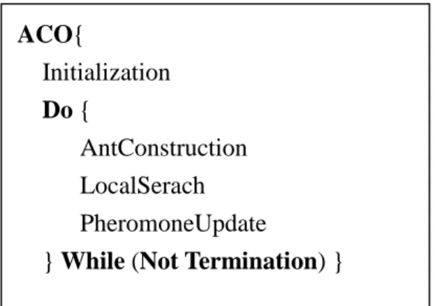
(13) 2.3 Ant Colony Optimization (ACO) Ant Colony Optimization (ACO), proposed by Dorigo et al. (1992), is a metaheuristic inspired by nature in which a colony of artificial ants cooperate in finding good solutions. The main idea of ACO is that the self-organizing principles, which allow the highly coordinated behavior of real ants, can be exploited to coordinate populations of artificial ants that collaborate to solve computational problems (Dorigo and Stützle, 2004). More specifically, the core behavior of artificial ants is the indirect communication between the ants via chemical pheromone trails which enable them to find short paths between food sources and their nest. In general,. 政治大. the ACO approach attempts to solve an optimization problem by iterating the. 立. following two steps (Blum, 2005): constructing candidate solutions using initial. ‧ 國. 學. pheromone trails and modifying the pheromone trails using the candidate solutions in a way that is deemed to bias future sampling toward high quality solutions.. ‧. Figure 2.3.1 presents the pseudo-code of the ACO algorithm for scheduling. y. Nat. and. n. al. LocalSearch,. PheromonUpdate.. er. AntConstruction,. io. Initialization,. sit. problems (Dorigo & Stützle 2004). The algorithm constitutes four major phases:. i n U. In. the. v. Initialization phase, an initial schedule is generated and pheromone trails are. Ch. engchi. calculated based on the initial schedule. In the AntConstruction phase, each artificial ant constructs a schedule using the pheromone trails. Once all artificial ants have constructed their own schedules, the schedules will be improved in the LocalSearch phase, an optional phase in early days, but a mandatory phase for most cases now. Then, in the PheromonUpdate phase, the pheromone trails are updated by applying properties of the schedules produced in the LocalSearch phase. The phases are iterated until a termination condition is satisfied.. 6.

(14) ACO{ Initialization Do { AntConstruction LocalSerach PheromoneUpdate } While (Not Termination) }. Figure 2.3.1 Pseudo-code for the general ACO algorithm. 政治大 Stützle (Stützle 1998a) proposed the first ACO algorithm, MAX-MIN Ant System 立. The ACO algorithm has been successfully applied to solve PFSP-makespan.. (MMAS), for PFSP-makespan. After that Ying and Liao (Ying & Liao 2004) applied. ‧ 國. 學. the Ant Colony System (ACS), developed by Dorigo and Gambardella (1997), for the. ‧. same problem and showed that ACS outperformed Genetic Algorithms, Simulated. sit. y. Nat. Annealing and Tabu Search. Rajendran and Ziegler (2004) developed two ACO. io. er. algorithms for PFSP-makespan: M-MMAS and PACO. The first algorithm, M-MMAS, modified the ideas of MMAS by incorporating the summation rule. al. n. v i n C h (2000) and U suggested by Merkle and Middendorf a newly proposed local search engchi. technique. The second was a newly developed ant colony algorithm called PACO. On average, both M-MMAS and PACO perform better than MMAS and the ACS of Ying and Liao (2004). 2.4 Particle Swarm Optimization (PSO) Particle swarm optimization (PSO) was proposed by Kennedy and Eberhart in 1995 ; it imitates the behavior of a swarm of birds searching for food. The searching process of PSO for an optimization problem starts with a population with randomly generated solutions (particles; the positions of the birds in the solution space). 7.

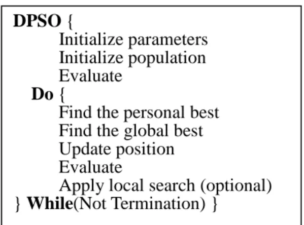
(15) Applying the swarm learning mechanism, each particle in the population searches the solution space by considering the effect of the best solution that all the particles have ever searched (global best), the effect of the best solution that the particle has ever searched (personal best) and the effect of searching the current neighborhood of its own. The new position of a particle in the next population is determined by its current position plus the effect of the global best solution and the effect of the personal best. This process will continue until a termination criterion is satisfied. The standard PSO equations for updating positions for birds are real-valued. 政治大 PFSP-makespan. Figure 2.4.1 presents the main components of DPSO (Pan et al., 立 equations; therefore, discrete PSO (DPSO) algorithms have been developed to solve. 2008a), which includes: (1) population initialization, (2) position update for particles,. ‧ 國. 學. and (3) a local search for improving the solution quality. A discrete position update. ‧. equation can be expressed as follows (Pan et al. 2008a):. sit. y. Nat. X it = c2 ⊗ F3 (c1 ⊗ F2 ( w ⊗ F1 ( X it −1 ), Pi t −1 ), G t −1 ). n. al. er. io. Given that the position of particle i in iteration t-1 is X it −1 , this equation first. Ch. i n U. v. implements function F1 with a probability of w; function F1 searches the neighborhood of X. t −1 i. engchi. . Then the equation implements function F2 with a probability of. c1. Function F2 exchanges information with the solution generated by function F1 and the personal best solution of particle i ( Pi t −1 ); it refers to the condition that particle i will learn from its personal best solution. Finally, this equation implements function F3 with a probability of c2. Function F3 exchanges information between the solution generated by functions F2 and the global best solution; it refers to the condition that particle i will learn from the global best solution. Figure 3 presents the pseudo-code for the DPSO algorithm with local search (Pan et al. 2008a). 8.

(16) DPSO { Initialize parameters Initialize population Evaluate Do { Find the personal best Find the global best Update position Evaluate Apply local search (optional) } While(Not Termination) } Figure 2.4.1 Pseudo-code for the general DPSO algorithm with local search. 政治大. There have been many PSO related algorithms proposed to solve the candidate. 立. problem recently. For example, a similar particle swarm optimization algorithm called. ‧ 國. 學. SPSOA (Lian et al., 2006) was proposed to solve PFSP-makespan. Computational experiments showed that SPSOA outperformed a basic GA. A discrete PSO version. ‧. called NPSO (Lian et al, 2008) was developed and successfully applied to the. Nat. sit. y. candidate problem, and the results showed that NPSO was more effective than a basic. n. al. er. io. GA. HPSO (Kuoa et al, 2009) is a continuous version of PSO which integrated the. i n U. v. random-key (RK) encoding scheme and the individual enhancement (IE) scheme into. Ch. engchi. PSO. The experimental results showed that HPSO was superior to a basic GA and NPSO. ATPPSO (Zhang C. et al., 2010) was proposed with the integration of PSO with genetic operators and annealing strategy. The results showed that both the solution quality and the convergence speed of ATPPSO outperform NPSO. Zhang J. et al. (2010) proposed a circular discrete particle swarm optimization algorithm (CDPSO). The particle similarity changes adaptively with the iterations and an order based strategy is introduced to preserve the swarm diversity. If the adjacent particles’ similarity is bigger than its current similarity threshold, the mutation operator is used to mutate the inferior. Furthermore, a fast makespan computation method based on 9.

(17) matrix is designed to improve the efficiency of the algorithm. The result showed that the solution quality and the stability of CDPSO precede both GA and SPSOA.. 立. 政治大. ‧. ‧ 國. 學. n. er. io. sit. y. Nat. al. Ch. engchi. 10. i n U. v.

(18) Chapter 3. The proposed metaheuristic (HLBS) Although there have been many metaheuristics based on GA, ACO, and PSO for solving PFSP-makespan, most of them follow the basic principles of evolutionary algorithms to improve the solutions iteration by iteration. In this research, we propose a population-based metaheuristic based on the local best solution, denoted as HLBS, to solve PFSP-makespan. The major idea of HLBS is based on the conjecture that the local best solution in an iteration possesses important information about the solution regions searched. Therefore, given a local best solution, we propose a simple. 政治大 search to promising solution 立regions. In addition, we propose a novel filter strategy to. approach to generate a trace-model based on the local best solution for guiding the. ‧ 國. 學. keep the search from trapping into local optimums and a new jump strategy to help the search escape if the search does become trapped at a local optimum. The basic. ‧. process of HLBS is presented as follows:. Set t = 0. Generate an initial solution using NEHT and let it be the local best. sit. y. Nat. 1.. do {. al. n. 2.. er. io. solution and the best-so-far solution.. Ch. engchi. i n U. v. 3.. Generate a trace-model based on the local best solution for iteration t.. 4.. Generate M new solutions according to the trace-model generated in Step 3 by applying a solution construction method.. 5.. Apply the filter strategy to the M solutions generated in Step 4; update the local best solution.. 6.. Launch the jump strategy if the search traps into a local optimum.. 7.. t=t+1. 8.. } while (Not Termination ). 9.. Return best-so-far solution 11.

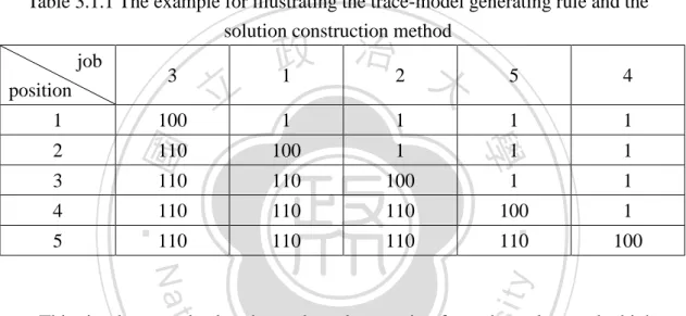
(19) The HLBS algorithm, different from general population-based metaheuristics, produces only a solution using the heuristic NEHT (Taillard 1990) in the initial iteration and sets the solution to be the local best solution and the best-so-far solution. The major loop in HLBS (step3~step7) generates a trace-model based on the local best solution, constructs M new solutions according to the trace-model by applying a solution construction method, and updates the local best solution with the solution produced by applying the new filter function and a local search method to the M new. 政治大 certain number of iterations, it is assumed that the search has trapped into a local 立. solutions. If the local best solution is not able to improve the best-so-far solution in a. optimum. Then the new jump strategy is launched to find a new initial solution as the. ‧ 國. 學. local best solution and the same loop (step3~step7) is performed on the new initial. ‧. solution. The major components of HLBS, trace-model generating rule, solution. sit. y. Nat. construction method, filter strategy and jump strategy are discussed in detail in the. io. n. al. er. following sections.. Ch. i n U. v. 3.1 Trace-model generating rule and solution construction method. engchi. The new trace-model generating rule is applied to generate a trace-model when the local best solution is updated in every iteration. The following example illustrates the procedure of the generating rule. Given the updated local best solution in an iteration is Π’ = (3, 1, 2, 5, 4), let τ(i, u) denote the trace-value of job u on position i, the generating rule first assigns a trace-value τl. to each job on its position in Π’, that is τ(1, 3) = τ(2, 1) = τ(3, 2) = τ(4, 5) = τ(5, 4) = τl. Then, for each job, the new rule assigns a trace-value τp to the positions prior to its position in Π’ and assigns a trace-value τs to the positions succeeded to its position in Π’. For instance, job 2 is on position 3 in Π’, so τ(1, 2) = τ(2, 2) = τp and τ(4, 2) = τ(5, 2) = τs. These three 12.

(20) trace-values, τl, τp, and τs, have to be properly determined to allow the trace-model to keep the sequence of the jobs in the local best solution while constructing new solutions and to keep the valuable information of the sequence of the jobs in every iteration. The following solution construction method will clearly illustrate this idea. A solution construction in an iteration is composed of job-selections from the first position to the last position for the solution. A revised job-selection rule based on the probabilistic action rule of Dorigo and Gambardella (1997) is proposed in HLBS. Given a parameter value q0 (0 ≤ q0 ≤ 1), an individual, individual k, first generates a. 政治大 to q , then equation (4) is used to select a job; otherwise, a probabilistic action rule 立. random number q from a uniform distribution ranged [0, 1]. If q is less than or equal 0. (equation (5)) is applied to select a job.. ‧ 國. 學. j = arg max{τ (i, u )} , if q ≤ q0. (4). u ∈S k ( i ). τ (i, j ) , if q > q0 ∑u∈S (i )τ (i, u ). ‧. Pk (i, j ) =. (5). k. io. y. sit. is the set of unscheduled jobs of individual k positioned on job i.. er. S k (i ). Nat. where. To better understand the solution construction method, the previous local best. al. n. v i n solution, Π’ = (3, 1, 2, 5, 4), is C used, and let τ = 1, τ U h e n g c h i = 100 and τ p. l. s. = 110; Table 3.1.1. summarizes the trace-values for all the jobs on different positions. The solution construction method for this example is presented as follows. Job selection for position 1: if q ≤ q0, since. S k (i ). = {1, 2, 3, 4, 5}, and τ(1, 3) = τl = 100 and τ(1, 1) =. τ(1, 2) = τ(1, 4) = τ(1, 5) = τp = 1, job 3 (j = arg max{τ (i, u )} = 3)) is selected for u ∈S k ( i ). position 1; if q > q0, each job j will be selected with a probability of τ(1, j)/(100 + 4×1), respectively, and a random number, between 0 and 1, is generated to select a job for position 1. Job selection for position 2 under the condition that job 5, not job 3, is selected for position 1: if q ≤ q0, since. S k (i ) =. 13. {1, 2, 3, 4}, and τ(2, 3) = 110, τ(2, 1).

(21) = 100 and τ(2, 2) = τ(2, 4) = 1, job 3 (j = arg max{τ (i, u )} = 3) is selected for position u ∈S k ( i ). 2; if q > q0, then job 3 has the highest probability, τ(2, 3)/ (110+100+1+1) = 110/(212), to be selected for position 2. This result shows that if job 3 is not selected for position 1, its position in Π’, it will be selected for position 2 with the highest probability. This illustrates the idea of the new trace-model generating rule which will keep a job on its position in the local best solution while constructing new solutions.. Table 3.1.1 The example for illustrating the trace-model generating rule and the solution construction method position 2 3 5. 5. 4. 1. 1. 1. 1. 110. 100. 1. 1. 1. 110. 110. 100. 1. 1. 110. 110. 110. 100. 1. 110. 110. 110. 110. 100. ‧. 4. 立. 100. 治政 1 2 大. 學. 1. 3. ‧ 國. job. sit. y. Nat. n. al. er. io. This simple example also shows that a large ratio of τl and τp values and a high q0. i n U. v. value will cause the job selection rule to highly retain the job sequence in the local. Ch. engchi. best solution and cause premature convergence. In order to investigate this problem, a study on the relationship among the τl, τp and τs values and a variable q0 setting method are considered in HLBS. The relationship among the τl, τp and τs values can be described using two simple equations: τl = τp×x and τs = τl＋τp×y = τp×x＋τp×y = τp×(x ＋y), so the relationship among the τl, τp and τs values can be determined by the two parameters x and y. As the values of these two parameters x and y become larger, there exists a higher possibility that the job sequence in the local best solution will be retained in constructing new solutions. Therefore, a number of the combinations of x and y will be considered in order to study the effect of the trace-model on the 14.

(22) performance of HLBS. The variable q0 setting method is to construct solutions using different q0 values. Given that there are M solutions constructed in a population and q0 varies from qhigh to qlow, the q0 for the k-th solution is calculated as follow: q0,k =qhigh – [ (qhigh–qlow)*k/M]. For example, if we set M to be equal to 10, k is between 0 to 9, and q0 varies from 0.96 (qhigh) to 0.66 (qlow), the set of q0,k is {0.96, 0.93, 0.90, …, 0.69}. Note that the higher the q0,k value, the higher the exploitative capability the individual has, and the lower the q0,k value, the higher the explorative capability the individual has. Therefore,. 政治大 exploitative capability and the explorative capability while searching the solution 立. including the solutions with different q0 values in a population may balance the. space.. ‧ 國. 學. In addition, a block property of PFSP-makespan is applied in the construction. ‧. method. Several recent works (Grabowski and Pempera, 2001, Grabowski and. sit. y. Nat. Wodecki, 2004, and Jin et al. 2007) have shown that the block property of the. io. er. PFSP-makespan can be developed and used to reduce the size of neighborhood. Therefore, the block property of PFSP-makespan will be considered in the. al. n. v i n C h the efficiency Uof HLBS. improve engchi. construction method to. A solution of a. PFSP-makespan problem can be presented as a PERT graph, and the length of the critical path of the graph is the makespan of the solution. A block is a sequence of consecutive jobs on a machine in a critical path; therefore, if a PFSP-makespan has m machines, the critical path of a solution will have m blocks. To apply the block property in the construction method for a PFSP-makespan problem with m machines, the HLBS will construct m solutions in each iteration. The first solution is constructed by choosing the first block from the local best solution and applying equations (4) and (5) to determine the jobs for the rest of the positions in the solution; the second solution is constructed by choosing the second block from the local best solution and 15.

(23) applying equations (4) and (5) to determine the jobs for the rest of the positions in the solution and so forth. Since the number of positions to be filled out while constructing a solution is decreased, applying the block property in the construction method will improve the efficiency of the HLBS.. 3.2 Filter strategy Local search methods are crucial for improving the effectiveness of population-based metaheuristics. They usually are applied to the best solution in an iteration or the global best solution to improve the quality of the solution; however,. 政治大. this may cause a search trap into local optima. The proposed filter strategy is applied. 立. when all the individuals (M) finish constructing their solutions in an iteration. It first. ‧ 國. 學. applies a filter function to find a solution from the M solutions, and then applies a local search method to the chosen solution. The purpose of the filter function is to. ‧. filter the solution regions that have been reviewed and guide the search to new. y. Nat. sit. solution regions in order to keep the search from trapping into local optima. We. n. al. er. io. define a filter-list as a first-in, first-out queue to store the makespan of the chosen. i n U. v. solution in each iteration and set a parameter called filter-size to define the size of the. Ch. engchi. queue. The queue is set to be empty initially. When all the M solutions are constructed, the solutions are sorted according to their makespans in ascending order, and the filter function is applied from the top of the M solutions until the first solution, whose makespan is different from all the makespans in the filter-list, is found and store the makespan of the solution in the filter list. If none of the M solutions has a different makespan from the makespans in the filter-list, the last of the M solutions is chosen (but the makespan will not be stored in the filter-list). The purpose of comparing makespans instead of job-sequences of solutions while using the filter function is two-fold. Firstly, it may guide the search to the solution regions which have not been 16.

(24) examined. Secondly, it can significantly reduce computation time by comparing the solution constructed by an individual and the solutions stored in the filter-list; this is especially critical when the number of jobs considered in a problem is large. In addition, the idea of choosing the solution with the largest makespan when none of the M solutions has a different makespan from the makespans in the filter-list is that it may prevent the search of HLBS from quick convergence. Once a solution is chosen using the filter function, the local search method (denoted as NEHT_LS) is applied to improve the makespan of the solution.. 政治大 Stützle’s (2007) iterative improvement method. Given that Π is the job sequence of 立. NEHT_LS integrates Taillard’s Modified-NEH method (Taillard 1990) with Ruiz and. the chosen solution, NEHT_LS first randomly chooses a job k and removes it from Π;. ‧ 國. 學. then it inserts job k into the first position, the last position, and the positions between. ‧. every two consecutive jobs in Π to generate n different solutions, and lets Π’’ be the. y. Nat. best of the n generated solutions. If the makespan of Π’’ is smaller than that of Π,. io. sit. NEHT_LS will update Π with Π’’ and will repeat the same procedure until Π cannot. er. be further improved. If the makespan of Π is smaller than that of the local best. al. n. v i n solution, it will update the localC solution with Π; if the h e n g c h i Umakespan of Π is smaller than. that of the best-so-far solution, it will update the best-so-far solution with Π. The procedure integrating the filter function and NEHT_LS is denoted as filtered local search (FLS). The filter strategy that implements FLS only once is denoted as F-Strategy1. The second filter strategy, denoted as F-Strategy2, first implements FLS, then determines if the makespan of the schedule generated by FLS dominates the best-so-far solution. If so, it will stop; otherwise, it will implement FLS one more time by using the filter function to find a solution different from the one found by the filter function in the first FLS. 17.

(25) 3.3 Jump strategy The main idea of the jump strategy is to guide the search to jump to another solution region when the search is trapped in a local optimum. We define the search trapped in a local optimum when the search is not able to improve the best-so-far solution in a number of iterations. The solution generated by the jump strategy is considered to be a new initial solution, and the search procedure is restarted. Two jump strategies are proposed in this research. The first jump strategy, J-Strategy1, defines two jumping distances: objective-value distance and sequence-. 政治大. structure distance. Objective-value distance implies that a threshold value is set to. 立. guarantee that a jump is far enough from the current local best solution. We set a. ‧ 國. 學. parameter, Jump-rate, to calculate the objective-value distance, objective-value distance = Jump-rate * objective value of the current local best solution. When a. ‧. local optimum is detected, an objective-value distance is calculated and the. y. Nat. sit. makespans of the M solutions constructed in the current iteration are compared with. n. al. er. io. the objective-value distance. Only the solutions that have makespans larger than the. i n U. v. objective-value distance are considered to be the candidates for a new initial solution.. Ch. engchi. If none of the M solutions has makespan larger than the objective-value distance, randomly choose a solution from the M solutions and use it as the new initial solution. If there is more than one candidate, a sequence-structure distance is applied to select a suitable one. A sequence-structure distance measures the structure similarity between two job-sequences, S1 and S2. Let (i, u1) be the job on position i in S1 and (i, u2) be the job on position i in S2, and define the distance between S1 and S2 on position i, d(i, u), be 0 if u1 = u2 and be 1 if u1 ≠ u2. The sequence-structure distance between S1 and S2 is then defined to be the sum of d(i, j) for all the positions. 18.

(26) The second jump strategy, J-Strategy2, first applies the Destruction and Construction Operation (Ruiz and Stützle, 2007) to the detected local optimum M times to generate M new solutions. The solution with the minimum makespan, which satisfies the following conditions: (i) the makespan is less than or equal to a pre-determined objective-value distance and (ii) the job sequence of the solution is different from the job sequence of the local optimum, is chosen and used as the new initial solution. If none of the M solutions satisfies the conditions, the same procedure will be implemented until a solution is produced. In order to apply the Destruction. 政治大 let the job sequence of the n jobs be s and the job sequence of the rest of the jobs in 立 and Construction Operation to a schedule, S, first randomly choose n1 jobs from S and 1. 1. S be s2. Then, insert the first job in s1 into the first position, the last position and the. ‧ 國. 學. positions between every two consecutive jobs in s2 and choose the sequence with the. ‧. smallest makespan; repeat the same process until all the n1 jobs in s1 are inserted in s2.. sit. y. Nat. In this research, the Destruction and Construction Operation is implemented three. io. n. al. er. times with n1 = 5 in J-Strategy2.. Ch. engchi. 19. i n U. v.

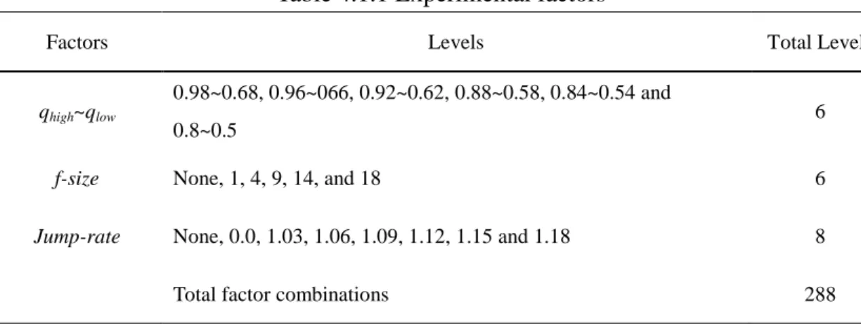
(27) Chapter 4. Computational experiments of HLBS Two HLBS-based metaheuristics are proposed by using different filter strategy, jump strategy, q0 setting method and trace-value. The basic HLBS, denoted as B-HLBS, is a HLBS that applies the filter strategy F-Startegy1, the jump strategy J-Strategy1, the variable q0 setting method and the trace-values, τp = 1, τl = 950 and τs = 1000, are determined by trial-and-error. The advanced HLBS, denoted as A-HLBS, is a HLBS using the filter strategy F-Startegy2, the jump strategy J-Strategy2, a fixed q0 method, and the trace-values are determined by properly studying the parameters x. 政治大 conducted for B-HLBS and立 A-HLBS respectively in the following sections. 4.1 Computational experiments of B-HLBS. 學. ‧ 國. and y; the block property is used as well. The computational experiments are. ‧. The well-known Taillard's test problems for PFSP-makespan (Taillard 1993) are. sit. y. Nat. used to evaluate the performance of B-HLBS. The test problems are composed of 12. io. er. different problem sets with different numbers of jobs and different numbers of machines. Twelve instances, selecting the first instance from each of the 12 problem. al. n. v i n sets, denoted as Test , are used C to investigate the effects h e n g c h i U of the three major factors of 1. B-HLBS: the variable q0 setting method, F-Startegy1 and J-Strategy1. Then, B-HLBS. with the best combination of the major factors will be applied to solve all the test problems, and its performance will be compared with promising population-based metaheuristics such as Genetic Algorithms (GA), Ant Colony Optimization (ACO) and Particle Swarm Optimization (PSO). Note that all the algorithms in this research are coded in C language and executed on the Linux operating system. The levels considered for the three major factors of B-HLBS are summarized in Table 4.1.1. Six levels are set for qhigh~qlow: 0.98~0.68, 0.96~066, 0.92~0.62, 0.88~0.58, 0.84~0.54, 0.8~0.5; six levels are set for the filter size (f-size) of 20.

(28) F-Startegy1: none, 1, 4, 9, 14, and 18, where none refers to no filter strategy is applied; eight levels are set for jump-rate of J-Strategy1: none, 0.0, 1.03, 1.06, 1.09, 1.12, 1.15 and 1.18, where none refers to no jump strategy is applied and 0.0 refers to the condition that only sequence-structure distance is considered. The remaining factors of B-HLBS are described as follows: the number of solutions (M) constructed in each iteration is set to be 10; the τ values used in the new pheromone generating rule, τp, τl, and τs, are set to be 1, 950, and 1000 respectively; the number of iterations without improvement for defining trapping at a local optimum is set to be the number of. 政治大 Therefore, there are a total of 288 different combinations of the three factors. B-HLBS 立. machines of the instances solved. All these factors are determined by trial-and-error.. is then applied with each of the 288 combinations to solve the 12 instances in Test1. ‧ 國. 學. with a limited computation time, n×(m/2)×30 milliseconds (Ruiz et al. 2006), for. ‧. three trials, where n refers to the number of jobs and m refers to the number of. sit. y. Nat. machines for the instances. The performance of B-HLBS with a combination of the. Heui − Best sol. i =1. Best sol. io. R. ARP = ∑ (. er. three factors for an instance is evaluated using Average Relative Performance (ARP):. ) , where Heu is the makespan obtained by any of R a× 100 iv l C n U factors, and Best is the best hcombination the three trials of B-HLBS with the e n g c hofi the. n. i. sol. makespan that all the research has found for the instance provided by Zobolas et al. (2009). Table 4.1.1 Experimental factors Factors. Levels. Total Levels. 0.98~0.68, 0.96~066, 0.92~0.62, 0.88~0.58, 0.84~0.54 and qhigh~qlow f-size Jump-rate. 6 0.8~0.5 None, 1, 4, 9, 14, and 18. 6. None, 0.0, 1.03, 1.06, 1.09, 1.12, 1.15 and 1.18. 8. Total factor combinations. 288 21.

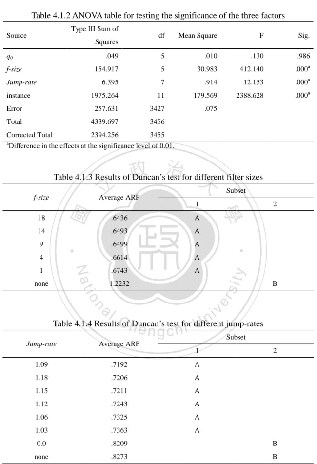
(29) The analysis of variance (ANOVA) is applied to analyze the ARPs produced by B-HLBS with all the 288 combinations. Table 4.1.2 presents the results of the ANOVA table. The results show that F-Startegy1 and J-Startegy1 significantly affect the ARP of the test problems. Therefore, the Duncan's test is applied to test if the performance of any two levels of F-Startegy1 and of the J-Startegy1 is significantly different. Table 4.1.3 presents the results of the Duncan's test for F-Startegy1. The results show that the major difference is between the level “none” and each of the other levels. This concludes that B-HLBS using F-Strategy1 significantly dominates. 政治大. B-HLBS without using F-Strategy1; however, the effect of the filter size is. 立. insignificant. Table 4.1.4 presents the results of the Duncan's test for J-Strategy1. The. ‧ 國. 學. results show that the major difference is between the level “none” and each of the other levels and between the level “0.0” and each of the other levels. This concludes. ‧. that B-HLBS using J-Strategy1 significantly dominates B-HLBS without using. y. Nat. sit. J-Strategy1; however, the effect of the jump-rate is insignificant. Therefore, the. n. al. er. io. condition that generates the best solution: qhigh~qlow = 0.98~0.68, f-size = 14 and. i n U. v. Jump-rate = 1.12, is considered to be the optimal condition for B-HLBS. Furthermore,. Ch. engchi. B-HLBS is applied to the same test problems under the condition: fixed q0 = 0.98, f-size = 14 and Jump-rate = 1.12, in order to evaluate the effect of the variable q0 setting method. Computational results show that the average ARP produced by B-HLBS using fixed q0 is 0.639, which is about 9% ((0.639-0.579)/0.639) worse than the average ARP produced by B-HLBS using variable q0 (qhigh~qlow = 0.98~0.68). This illustrates that using different q0 values for the M solutions constructed in an iteration is able to improve the explorative capability for B-HLBS.. 22.

(30) Table 4.1.2 ANOVA table for testing the significance of the three factors Type III Sum of Source. df. Mean Square. F. Sig.. .049. 5. .010. .130. .986. 154.917. 5. 30.983. 412.140. .000a. 6.395. 7. .914. 12.153. .000a. 1975.264. 11. 179.569. 2388.628. .000a. Error. 257.631. 3427. .075. Total. 4339.697. 3456. Corrected Total. 2394.256. 3455. Squares q0 f-size Jump-rate instance. Difference in the effects at the significance level of 0.01.. 政治大. Table 4.1.3 Results of Duncan’s test for different filter sizes. 立. f-size. Subset. Average ARP 1. Nat. 1 none. A. .6499. A. .6614. A. .6743. A. y. 4. .6493. ‧. 9. A. sit. 14. .6436. 1.2232. B. io. er. 18. 2. 學. ‧ 國. a. al. n. v i n Table 4.1.4 ResultsC ofhDuncan’s test for different e n g c h i U jump-rates Subset Jump-rate. Average ARP 1. 2. 1.09. .7192. A. 1.18. .7206. A. 1.15. .7211. A. 1.12. .7243. A. 1.06. .7325. A. 1.03. .7363. A. 0.0. .8209. B. none. .8273. B. 23.

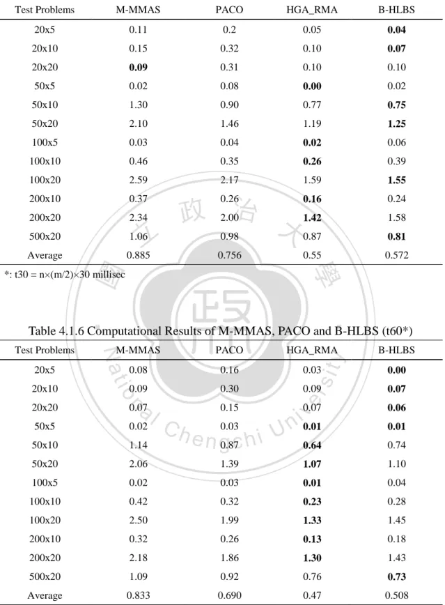
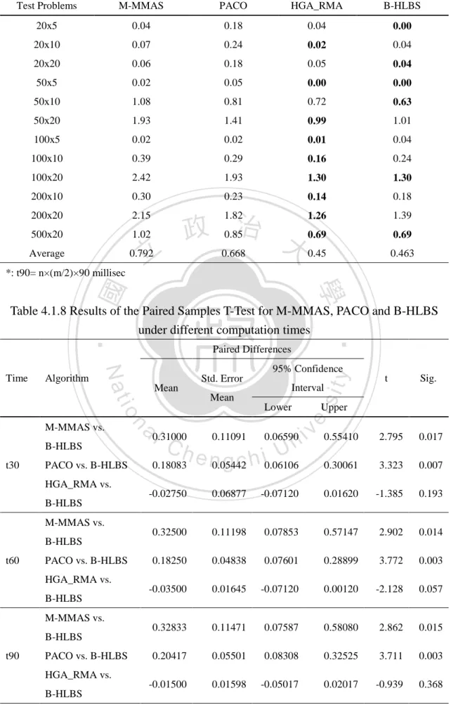
(31) B-HLBS with the optimal condition is then applied to solve the test problems in all the problem sets, and its performance is compared with two ACO algorithms, M-MMAS and PACO (Rajendran & Ziegler 2004), a PSO algorithm, PSOvns. and. two hybrid GA related metaheuristics, NEGAvns (Zobolas 2009) and HGA_RMA (Ruiz et al. 2006), which reported very promising solutions for PFSP-makespan. Ruiz et al. (2006) compared the performance of M-MMAS, PACO and HGA_RMA based on the same number of replication runs (R=5) and the same computation times: n×(m/2)×30, n×(m/2)×60, and n×(m/2)×90 milliseconds. All the. 政治大 compare the performance of B-HLBS with M-MMAS, PACO and HGA_RMA based 立 algorithms were run on a PC with Intel Pentium IV at 2.8 GHz. Therefore, we. on the same computation times using a PC with the same computing power. Tables. ‧ 國. 學. 4.1.5 to 4.1.7 present the average ARPs produced by M-MMAS, PACO, HGA_RMA. ‧. and B-HLBS for the twelve problem sets with each of the three computation times,. sit. y. Nat. respectively. The Paired Samples T-test is applied to test if the performance of. io. er. B-HLBS significantly dominates M-MMAS, PACO and HGA_RMA respectively. Table 4.1.8 summarizes the results of all the Paired Samples T-tests. The results show. al. n. v i n C h M-MMAS andUPACO under all the different that B-HLBS significantly dominates engchi. computation times, but the difference of the performance between B-HLBS and HGA_RMA is insignificant.. 24.

(32) Table 4.1.5 Computational Results of M-MMAS, PACO and B-HLBS (t30*) Test Problems. M-MMAS. PACO. HGA_RMA. B-HLBS. 20x5. 0.11. 0.2. 0.05. 0.04. 20x10. 0.15. 0.32. 0.10. 0.07. 20x20. 0.09. 0.31. 0.10. 0.10. 50x5. 0.02. 0.08. 0.00. 0.02. 50x10. 1.30. 0.90. 0.77. 0.75. 50x20. 2.10. 1.46. 1.19. 1.25. 100x5. 0.03. 0.04. 0.02. 0.06. 100x10. 0.46. 0.35. 0.26. 0.39. 100x20. 2.59. 2.17. 1.59. 1.55. 200x10. 0.37. 0.26. 0.16. 0.24. 200x20. 2.34. 2.00. 1.42. 1.58. 500x20. 1.06. 0.98. 0.87. 0.81. Average. 0.885. 0.756. 0.55. 0.572. 立. 政治大. ‧ 國. 學. *: t30 = n×(m/2)×30 millisec. ‧. Table 4.1.6 Computational Results of M-MMAS, PACO and B-HLBS (t60*) 0.08. 0.16. 0.03. 0.00. 0.09. 0.30. 0.09. 0.07. 0.07 v i n 0.01. 0.06. 0.64. 0.74. sit. B-HLBS. 20x20. n. al. y. HGA_RMA. io. 20x10. PACO. er. 20x5. M-MMAS. Nat. Test Problems. 50x5. 0.02. 50x10. 1.14. 50x20. 2.06. 1.39. 1.07. 1.10. 100x5. 0.02. 0.03. 0.01. 0.04. 100x10. 0.42. 0.32. 0.23. 0.28. 100x20. 2.50. 1.99. 1.33. 1.45. 200x10. 0.32. 0.26. 0.13. 0.18. 200x20. 2.18. 1.86. 1.30. 1.43. 500x20. 1.09. 0.92. 0.76. 0.73. Average. 0.833. 0.690. 0.47. 0.508. 0.07. 0.15. Ch. e n g0.87c h i U 0.03. *: t60= n×(m/2)×60 millisec. 25. 0.01.

(33) Table 4.1.7 Computational Results of M-MMAS, PACO and B-HLBS (t90*) Test Problems. M-MMAS. PACO. HGA_RMA. B-HLBS. 20x5. 0.04. 0.18. 0.04. 0.00. 20x10. 0.07. 0.24. 0.02. 0.04. 20x20. 0.06. 0.18. 0.05. 0.04. 50x5. 0.02. 0.05. 0.00. 0.00. 50x10. 1.08. 0.81. 0.72. 0.63. 50x20. 1.93. 1.41. 0.99. 1.01. 100x5. 0.02. 0.02. 0.01. 0.04. 100x10. 0.39. 0.29. 0.16. 0.24. 100x20. 2.42. 1.93. 1.30. 1.30. 200x10. 0.30. 0.23. 0.14. 0.18. 200x20. 2.15. 1.82. 1.26. 1.39. 500x20. 1.02. 0.85. 0.69. 0.69. Average. 0.792. 0.668. 0.45. 0.463. 立. *: t90= n×(m/2)×90 millisec. 政治大. ‧ 國. 學. Mean. PACO vs. B-HLBS. y. t. Sig.. Interval. Mean Lower. Upper. a 0.31000 0.11091 0.06590 i v 0.55410 l C hengchi Un. n. B-HLBS. sit. io M-MMAS vs.. t30. 95% Confidence Std. Error. er. Algorithm. Paired Differences. Nat. Time. ‧. Table 4.1.8 Results of the Paired Samples T-Test for M-MMAS, PACO and B-HLBS under different computation times. 2.795. 0.017. 0.18083. 0.05442. 0.06106. 0.30061. 3.323. 0.007. -0.02750. 0.06877. -0.07120. 0.01620. -1.385. 0.193. 0.32500. 0.11198. 0.07853. 0.57147. 2.902. 0.014. 0.18250. 0.04838. 0.07601. 0.28899. 3.772. 0.003. -0.03500. 0.01645. -0.07120. 0.00120. -2.128. 0.057. 0.32833. 0.11471. 0.07587. 0.58080. 2.862. 0.015. 0.20417. 0.05501. 0.08308. 0.32525. 3.711. 0.003. -0.01500. 0.01598. -0.05017. 0.02017. -0.939. 0.368. HGA_RMA vs. B-HLBS M-MMAS vs. B-HLBS t60. PACO vs. B-HLBS HGA_RMA vs. B-HLBS M-MMAS vs. B-HLBS. t90. PACO vs. B-HLBS HGA_RMA vs. B-HLBS. 26.

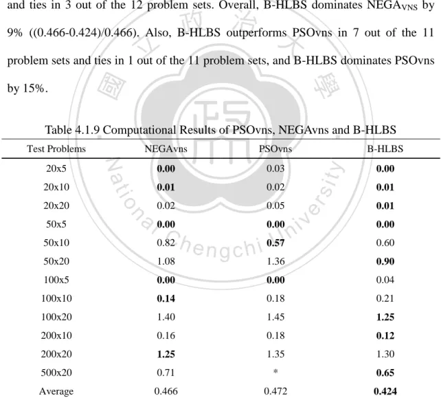
(34) Table 4.1.9 presents the average ARPs generated by NEGAvns, PSOvns, and B-HLBS, on a PC with Intel Pentium IV at 2.4 GHz under the same computation time, n×m/10 seconds, and the same number of replication runs (R=10) (Zobolas et al. 2009). The Paired Samples T-test is applied to compare the performance between B-HLBS and each of algorithms: NEGAvns and PSOvns. These tests show that B-HLBS does not significantly dominate any of NEGAvns and PSOvns. However, the results show that B-HLBS is superior to NEGAVNS in 6 out of the 12 problem sets and ties in 3 out of the 12 problem sets. Overall, B-HLBS dominates NEGAVNS by. 政治大. 9% ((0.466-0.424)/0.466). Also, B-HLBS outperforms PSOvns in 7 out of the 11. 立. problem sets and ties in 1 out of the 11 problem sets, and B-HLBS dominates PSOvns. ‧. ‧ 國. 學. by 15%.. 50x10. 0.03. 0.00. 0.01. 0.02. 0.01. 0.02. 0.05. a l 0.00 C 0.82 h. n. 50x5. io. 20x20. 0.00. y. 20x10. PSOvns. Nat. 20x5. NEGAvns. 50x20. 1.08. 100x5. i n 0.57 U 0.00. engchi. er. Test Problems. sit. Table 4.1.9 Computational Results of PSOvns, NEGAvns and B-HLBS. v. B-HLBS. 0.01 0.00 0.60. 1.36. 0.90. 0.00. 0.00. 0.04. 100x10. 0.14. 0.18. 0.21. 100x20. 1.40. 1.45. 1.25. 200x10. 0.16. 0.18. 0.12. 200x20. 1.25. 1.35. 1.30. 500x20. 0.71. *. 0.65. Average. 0.466. 0.472. 0.424. *: The authors do not provide results for the 500 × 20 instance group.. 27.

(35) 4.2 Computational experiments of A-HLBS The same procedure of data analysis used for B-HLBS is used for A-HLBS. Table 4.2.1 summarizes the levels considered for the major factors of A-HLBS. Three levels are set for x: 1, 50, 100 and six levels are set for y: 1, 50, 100, 200, 400, 600; four levels are set for q0: 0.0, 0.7, 0.8, 0.9; two levels are set for the f-size of F-Startegy2: none and 7, where none refers to no filter strategy is applied; two levels are set for jump-rate of J-Strategy2: none and 1.02, where none refers to no jump strategy is applied. The f-size with 7 and the jump-rate with 1.02 are determined by trial-and-error. The remaining factors of A-HLBS are the number of the solutions (M). 政治大. constructed in each iteration, the number of iterations without improvement for. 立. defining trapping at a local optimum, and the termination criterion. The first two. ‧ 國. 學. factors are determined by trial-and-error and set to be the number of machines of the instances solved, and the execution time, like most of the other researches, is chosen. ‧. to be the termination criterion. Therefore, there are a total of 288 different. y. Nat. er. io. al. sit. combinations of the five factors.. n. Table 4.2.1 Experimental factors. Factors. C Levels hengchi. i n U. v. Total Levels. x. 1, 50 and 100. 3. y. 1, 50, 100, 200, 400 and 600. 6. q0. 0.0, 0.7, 0.8 and 0.9. 4. None and 7. 2. None and 1.02. 2. f-size Jump-rate. Total factor combinations. 288. The A-HLBS is applied with each of the 288 combinations to solve the 12 28.

(36) instances in Test1 with limited computation times, n×(m/2)×30 milliseconds (Ruiz et al. 2006), for three trials, and the analysis of variance (ANOVA) is applied to analyze the ARPs produced. Table 4.2.2 presents the results of the ANOVA table. The results show that all the factors significantly affect the ARP of the test problems. Therefore, the Duncan’s test is applied to test all the factors. Table 4.2.3 summarizes the results of the Duncan's test for all the five factors; the minimum average ARP for each factor is: q0 = 0.9, x = 50, y = 400, f-size = 7 and jump-rate =1.02. This condition is very close to the condition that generates the best solution: q0 = 0.8, x = 50, y = 400, f-size. 政治大 (0.5985) and the average ARP of q = 0.9 (0.5981) is negligible, the optimal 立 = 7 and jump-rate =1.02. Since the difference between the average ARP of q0 = 0.8 0. combination of the five factors for A-HLBS is determined to be q0 = 0.9, x = 50, y =. ‧ 國. 學. 400, f-size = 7 and jump-rate =1.02.. ‧. Table 4.2.2 ANOVA table for testing the significance of the five factors Mean. x. .254. 3. .136. 1. .264. er. a.264 l 1.712C h. n. Jump-rate. io. f-size. .407. Square. iv. 1.712 n U e n g2 c h i .127 1. F. Sig.. 9.129. .000a. 17.741. .000a. 115.089. .000a. 8.527. .000a. sit. df. Squares. q0. y. Nat. Type III Sum of Source. .256. 5. .051. 3.443. .004a. 1627.599. 11. 147.964. 9948.798. .000a. Error. 51.042. 3432. .015. Total. 2950.158. 3456. Corrected Total. 1681.534. 3455. y instance. a. Difference in the effects at the significance level of 0.01.. 29.

(37) Table 4.2.3 Results of Duncan’s test for the five major factors Subset q0. Average ARP. .90. .5981. A. .80. .5985. A. .70. .6025. A. 0.0. .6244. x. Average ARP. 1. 2. B Subset 1. 50. .5972. A. 100. .6029. A. 1. .6175. y. Average ARP. A. .5971. A. .6026. A. .6064. A. .6109. A. B. Subset. Average ARP 1. Jump-rate. Average ARP. n. none. a l.5970 C .6150 h. 7. B. y. .5966. 2. .6216. io. f-size. Nat. 1. 1. sit. 50. Subset. ‧. 100. B. i n U. A. engchi. .5840. none. .6280. v. 2. B Subset. 1 1.02. er. 600. ‧ 國. 200. 政治大. 學. 400. 立. 2. 2. A B. 30.

(38) The A-HLBS with the optimal combination of the five factors is then applied to solve the test problems in all the problem sets. Since the analysis in Section 4.1 has shown that B-HLBS significantly dominates M-MMAS and PACO, the performance of A-HLBA is first compared only with HGA_RMA and B-HLBS under different computation times: n×(m/2)×30, n×(m/2)×60, and n×(m/2)×90 milliseconds, and then with NEGAvns, PSOvns and B-HLBS under the same computation time, n×m/10 seconds. Tables 4.2.4 to 4.2.6 present the average ARPs produced by HGA_RMA,. 政治大 times, respectively. The Paired Samples T-test is applied to test if the performance of 立. B-HLBS and A-HLBS for the twelve problem sets with each of the three computation. A-HLBS significantly dominates HGA_RMA and B-HLBS, respectively. Table 4.2.7. ‧ 國. 學. summarizes the results of all the Paired Samples T-tests. The results show that. ‧. A-HLBS significantly dominates HGA_RMA and B-HLBS under all the different. sit. y. Nat. computation times.. io. er. Table 4.2.8 presents the average ARPs generated by NEGAvns, PSOvns, B-HLBS and A-HLBS. The Paired Samples T-test is also applied to compare the. al. n. v i n performance between A-HLBS C and each of the algorithms: h e n g c h i U HGA_RMA, NEGAvns, PSOvns and B-HLBS. Table 4.2.9 summarizes the results of all the Paired Samples. T-tests. The results show that A-HLBS significantly dominates NEGAvns, PSOvns and B-HLBS.. 31.

(39) Table 4.2.4 Computational Results of HGA_RMA, B-HLBS and A-HLBS (t30*) Test Problems. HGA_RMA. B-HLBS. A-HLBS. 20x5. 0.05. 0.04. 0.04. 20x10. 0.10. 0.07. 0.00. 20x20. 0.10. 0.10. 0.02. 50x5. 0.00. 0.02. 0.00. 50x10. 0.77. 0.75. 0.61. 50x20. 1.19. 1.25. 1.01. 100x5. 0.02. 0.06. 0.04. 100x10. 0.26. 0.39. 0.22. 100x20. 1.59. 1.55. 1.36. 200x10. 0.16. 0.24. 0.11. 200x20. 1.42. 500x20. 0.87. 立 *: t30 = n×(m/2)×30 millisec Average. 0.55. 政治大 1.58. 1.35. 0.81. 0.64. 0.57. 0.45. ‧ 國. 學. Table 4.2.5 Computational Results of HGA_RMA, B-HLBS and A-HLBS (t60*). 50x20 100x5. 0.07. 0.07. 0.06. 0.01. 0.01. a l 0.64 1.07 Ch 0.01. y. 0.09. n. 50x10. io. 50x5. 0.00. sit. 20x20. 0.03. Nat. 20x10. B-HLBS. er. 20x5. HGA_RMA. ‧. Test Problems. iv 1.10 n engchi U 0.74. A-HLBS 0.03 0.00 0.01 0.00 0.60 0.84. 0.04. 0.04. 100x10. 0.23. 0.28. 0.19. 100x20. 1.33. 1.45. 1.09. 200x10. 0.13. 0.18. 0.09. 200x20. 1.30. 1.43. 1.24. 500x20. 0.76. 0.73. 0.55. Average. 0.47. 0.51. 0.39. *: t60= n×(m/2)×60 millisec. 32.

(40) Table 4.2.6 Computational Results of HGA_RMA, B-HLBS and A-HLBS (t90*) Test Problems. HGA_RMA. B-HLBS. A-HLBS. 20x5. 0.04. 0.00. 0.03. 20x10. 0.02. 0.04. 0.00. 20x20. 0.05. 0.04. 0.00. 50x5. 0.00. 0.00. 0.00. 50x10. 0.72. 0.63. 0.55. 50x20. 0.99. 1.01. 0.74. 100x5. 0.01. 0.04. 0.04. 100x10. 0.16. 0.24. 0.16. 100x20. 1.30. 1.30. 1.00. 200x10. 0.14. 0.18. 0.07. 200x20. 1.26. 500x20. 0.69. 立. Average. 0.45. 政治大 1.39. 1.09. 0.69. 0.49. 0.46. 0.35. *: t90= n×(m/2)×90 millisec. ‧ 國. 學. io. n. al. B-HLBS vs. A-HLBS t30. HGA_RMA vs. A-HLBS B-HLBS vs. A-HLBS. 95% Confidence. Error. Interval. Mean. Lower. sit. Mean. Std.. t. Sig.. 0.17426. 5.092. 0.000. 0.14945. 3.749. 0.003. er. Algorithm. y. Paired Differences. Nat. Time. ‧. Table 4.2.7 Results of the Paired Samples T-Test for HGA_RMA, B-HLBS and A-HLBS under different computation times. 0.12167 0.02389 0.06907 i v n C U h e n0.02512 0.09417 0.03888 gchi. Upper. 0.11750. 0.03305. 0.04475. 0.19025. 3.555. 0.005. HGA_RMA vs. A-HLBS. 0.08250. 0.02669. 0.02376. 0.14124. 3.091. 0.010. B-HLBS vs. A-HLBS. 0.11583. 0.03491. 0.03899. 0.19268. 3.318. 0.007. HGA_RMA vs. A-HLBS. 0.10083. 0.03223. 0.02990. 0.17176. 3.129. 0.010. t60. t90. 33.

(41) Table 4.2.8 Computational Results of HGA_RMA, NEGAvns, PSOvns, B-HLBS and A-HLBS (t=n×m/10 seconds) Test Problems. NEGAvns. PSOvns. B-HLBS. A-HLBS. 20x5. 0.00. 0.03. 0.00. 0.00. 20x10. 0.01. 0.02. 0.01. 0.00. 20x20. 0.02. 0.05. 0.01. 0.00. 50x5. 0.00. 0.00. 0.00. 0.00. 50x10. 0.82. 0.57. 0.6. 0.56. 50x20. 1.08. 1.36. 0.9. 0.67. 100x5. 0.00. 0.00. 0.04. 0.04. 100x10. 0.14. 0.18. 0.21. 0.13. 100x20. 1.40. 1.45. 1.25. 0.92. 200x10. 0.16. 0.18. 0.12. 0.05. 200x20. 1.25. 1.35. 1.30. 1.01. 500x20. 0.71. *. 0.65. 0.46. Average. 0.466. 0.472. 0.424. 0.324. *: The authors do not provide results for the 500 × 20 instance group.. 學. ‧ 國. 立. 政治大. B-HLBS vs. A-HLBS. Mean. Lower. 34. y t. Sig.. Upper. 0.051 0.033 0.258 a0.146 v i l n 0.16455 C h0.07383 0.00003U 0.32906 e n g c 0.026 hi 0.104 0.035 0.182. n. PSOvns vs. A-HLBS. 95% Confidence Interval. Mean. er. io NEGA_VNS vs. A-HLBS. Std. Error. sit. Paired Differences. Nat. Algorithm. ‧. Table 4.2.9 Results of the Paired Samples T-Test for NEGAvns, PSOvns, B-HLBS and A-HLBS (t=n×m/10 seconds). 2.851. 0.016. 2.229. 0.050. 2.947. 0.013.

(42) Chapter 5. Conclusions and further research This research proposes two population-based metaheuristics based on the local best solution, B-HLBS and A-HLBS, for the permutation flow shop scheduling problem (PFSP-makespan). The computational results in Chapter 4 have shown that A-HLBS is an effective heuristic for PFSP-makespan. It dominates all the promising population-based metaheuristics related to ACO, PSO and GA (M-MMAS, PACO, PSOvns, HGA_RMA, and NEGAvns). However, our results demonstrate that the operation of A-HLBS can be further improved. Our analyses illustrate that the. 政治大 the filter strategy, and the 立 jump strategy. With proper selection of x, y and q. performance of HLBS is highly influenced by the three major factors: the trace-model, 0. of the. ‧ 國. 學. trace-model and application of different filter strategy and jump strategy, A-HLBS significantly dominates B-HLBS. Therefore, further studies on the interaction of these. ‧. three factors are worthwhile. For instance, the path relinking method (Glover, 1996). sit. y. Nat. can be applied to the solutions in the populations generated by J-Startegy1 and. n. al. er. io. J-Strategy2 to produce new initial solutions. Since the path relinking has been proved. i n U. v. to be effective for generating promising solutions for PFSP-makespan (Nowicki and. Ch. engchi. Smutnicki, 1996), it is believed that the method is able to produce effective initial solutions and improve the performance of HLBS. In addition, since the flow shop problem is a special case of the job shop problem, the proposed heuristic can also be applied towards job shop problems. It is important to note that although computation time needed in a PC is a major termination criterion used to compare the performance of most of the metaheuristics developed for PFSP–makespan, this criterion is inappropriate because the computation time using a PC is affected by several factors of the PC such as the level of CPU, the size of memory and the operating system. It is very difficult to find equal 35.

(43) computing-power machines when comparing the performance of different metaheuristics. In addition, the coding skill of the computer program will also significantly affect the performance of the metaheuristics, given computation time as the termination criterion, because it will affect the number of solutions searched in a limited computation time. Therefore, it is believed that the number of solutions searched using a metaheuristic could be a more appropriate metric to evaluate its effectiveness. Assuming analysis under this new criterion, the effectiveness of A-HLBS may be comparable or even better than the current optimal metaheuristics.. 政治大 future studies considering this criterion is warranted. 立. Therefore in order to more accurately assess the effectiveness of metaheuristics,. ‧. ‧ 國. 學. n. er. io. sit. y. Nat. al. Ch. engchi. 36. i n U. v.

(44) References Andreas, N. & Omirou, S. (2006). Differential evolution for sequencing and scheduling optimization. Journal of Heuristics, 12(6), 395-411. Blum, C (2005). Ant colony optimization: Introduction and recent trends. Physics of Life Reviews, 2(4), 353-373. Chen, C. L., Vempati, V. S. & Aljaber, N. (1995). An application of genetic algorithms for flow shop problems. European Journal of Operational Research, 80(2), 389-396.. 政治大 Continuous Flow Shop 立Problem. Computers & Industrial Engineering, 30(4),. Chen, C. L., Neppalli, V. R. & Aljaber, N. (1996). Genetic Algorithms Applied to the. ‧ 國. 學. 919-929.. Chen, Y. M., Chen, M. C., Chang, P. C. & Chen, S. H. (2012), Extended Artificial. ‧. Chromosomes Genetic Algorithm for Permutation Flowshop Scheduling. sit. y. Nat. problems, Computers & Industrial Engineering, 62(2), 536–545.. n. al. er. io. Dorigo, M. (1992) Optimization, Learning and Natural Algorithm. Ph.D. Thesis, DEI, Politecnico di Milano, Italy.. Ch. engchi. i n U. v. Dorigo, M. & Gambardella, L. M. (1997). Ant colony system: a cooperative learning approach to the travelling salesman problem. IEEE T Evolut Comput,1,53–66. Dorigo, M. & Stützle, T. (2004). Ant colony optimization. MIT, Cambridge. Framinan, J., Gupta, J. N. D. & Leisten, R. (2004). A review and classification of heuristics for the permutation flowshop with makespan objective. Journal of Operational Research Society, 55, 1243–1255. Garey, M. R., Johnson, D. S. & Sethi, R. (1976). The complexity of flowshop and jobshop scheduling. Mathematics of Operations Research, 1(2), 117-129.. 37.

(45) Glover, F. (1996), Tabu Search and Adaptive memory programming - Advances, applications and challenges. Interfaces in Computer Science and Operations Research. Barr, Helgason and Kennington, eds., Kluwer Academic Publishers, 1-75. Grabowski, J. & Pempera, J. (2001). New block properties for the permutation flow shop problem with application in tabu search. Journal of the Operational Research Society, 52, 210-220. Grabowski, J. & Wodecki, M. (2004). A very fast tabu search algorithm for the. 政治大 Operations Research, 31(11), 1891-1909. 立. permutation flowshop problem with makespan criterion. Computers &. Graham, R. L., Lawler, E. L., Lenstra, J. K. & Rinnooy Kan, A.H.G. (1979).. ‧ 國. 學. Optimization and approximation in deterministic sequencing and scheduling : a. ‧. survey. Annals of Discrete Mathematics, 5, 287-326.. sit. y. Nat. Hejazi, S. R. & Saghafian, S. (2005). Flowshop scheduling problems with makespan. io. 2895–2929.. er. criterion: a review. International Journal of Production Research, 43(14),. al. n. v i n C h An improved version Jin, F., Song, S.J. & Wu, C. (2007). of the NEH algorithm and engchi U. its application to large-scale flow-shop scheduling problems. IIE Transactions, 39,. 229-234. Kennedy, J. & Eberhart, R. (1995). Particle swarm optimization. In Proceedings of IEEE international conference on neural network, 1942–1948. Kuo, I. H., Horng, S. J., Kao, T. W., Lin, T. L., Lee, C. L., Terano, T. & Pan, Y. (2009). An efficient flow-shop scheduling algorithm based on a hybrid particle swarm optimization model. Expert Systems with Applications, 36(3), 7027–7032.. 38.

(46) Lian, Z., Gu, X. & Jiao, B. (2006). A similar particle swarm optimization algorithm for permutation flowshop scheduling to minimize makespan. Applied Mathematics and Computation, 175(1), 773–785. Lian, Z., Gu, X. & Jiao, B. (2008). A novel particle swarm optimization algorithm for permutation flow-shop scheduling to minimize makespan. Chaos, Solitons and Fractals, 35, 851–861. Liao, C. J., Tseng, C. T. & Luarn, P. (2007). A discrete version of particle swarm optimization for flowshop scheduling problems. Computers & Operations. 政治大 Lin, S. W & Ying, K. C. (2011). Minimizing makespan and total flowtime in 立 Research, 34(10), 3099-3111.. permutation flowshops by a bi-objective multi-start simulated-annealing. ‧ 國. 學. algorithm. Computers & Operations Research, doi:10.1016/j.cor.2011.08.009.. flowshop. scheduling. problem.. Applied. Soft. Computing. sit. y. Nat. permutation. ‧. Liu, Y. F. & Liu, S. Y. (2011). A hybrid discrete artificial bee colony algorithm for. io. er. doi:10.1016/j.asoc.2011.10.024.. Merkle, D. & Middendorf, M. (2000). An ant algorithm with a new pheromone. al. n. v i n C h problems. In: Proceedings evaluation rule for total tardiness of the EvoWorkshops, engchi U 1803(LNCS), 287–296.. Nowicki, E. & Smutnicki, C. (1996). A fast tabu search algorithm for the permutation flowshop problem. European Journal of Operational Research, 91, 160-175. Ogbu, F. & Smith, D. (1990). The application of the simulated annealing algorithm to the solution of the n/m/Cmax flowshop problem. Computers & Operations Research, 17(3), 243-253. Onwubolu, G. & Davendra, D. (2006). Scheduling flow shops using differential evolution algorithm. European Journal of Operational Research, 171(2), 674-692. 39.

(47) Osman, I. & Potts, C. (1989). Simulated annealing for permutation flow shop scheduling. OMEGA, 17(6), 551-557. Pan, Q. K., Tasgetiren, M. F. & Liang, Y. C. (2008a). A discrete particle swarm optimization algorithm for the no-wait flowshop scheduling problem. Computer & Operations Research, 35(9), 2807-2839. Pan, Q. K., Tasgetiren, M. F. & Liang, Y. C. (2008b). A Discrete differential evolution algorithm for the permutation flowshop scheduling problem. Computers & Industrial Engineering. 55(4), 795-816.. 政治大 scheduling to minimize makespan/total flowtime of jobs. European Journal of 立. Rajendran, C. & Ziegler, H. (2004). Ant-colony algorithms for permutation flowshop. Operational Research, 155(2), 426–438.. ‧ 國. 學. Rameshkumar, K., Suresh, R. K. & Mohanasundaram, K. M. (2005). Discrete particle. ‧. swarm optimization (DPSO) algorithm for permutation flowshop scheduling to. sit. y. Nat. minimize makespan. In Proceedings of the ICNC (3), 572–581.. io. er. Reeves, C. R. (1993). Improving the efficiency of tabu search for machine sequencing problem. Journal of the Operational Research Society, 44(4), 375–382.. al. n. v i n C algorithm Reeves, C. R. (1995). A genetic flowshop sequencing. Computers & U h e n g for i h c Operations Research. 22(1), 5–13.. Reeves, C. R. & Yamada, T. (1998). Genetic algorithms, path relinking and the flowshop sequencing problem. Evolutionary Computation, 6(1), 45–60. Ruiz, R. & Maroto, C. (2005). A comprehensive review and evaluation of permutation flowshop heuristics. European Journal of Operational Research 165, 479–494. Ruiz, R., Maroto, C. & Alcaraz, J. (2006). Two new robust genetic algorithms for the flowshop scheduling problem. OMEGA, 34, 461–47.. 40.

(48) Ruiz, R. & Stützle, T. (2007). A simple and effective iterated greedy algorithm for the permutation flowshop scheduling problem. European Journal of Operational Research,. 177(3),2033-2049.. Stützle, T. (1998a). An ant approach to the flow shop problem. In: Proceedings of the 6th European Congress on Intelligent Techniques & Soft Computing, Aachen, Germany, 3, 1560-1564. Stützle, T. (1998b). Applying iterated local search to the permutation flowshop problem. Technical Report, AIDA-98-04, FG Intellektik, TU Darmstadt.. 政治大 problem. European Journal of Operational Research, 47(1), 65–74. 立. Taillard, E. (1990). Some efficient heuristic methods for the flow shop sequencing. Operational Research, 64(2), 278-285.. 學. ‧ 國. Taillard, E. (1993). Benchmarks for basic scheduling problems. European Journal of. ‧. Tasgetiren, M. F., Sevkli, M., Liang, Y. C. & Gencyilmaz, G. (2004). Particle swarm. sit. y. Nat. optimization algorithm for permutation flowshop sequencing problem. In. io. LNCS 3172, Springer-Verlag, 381-89.. al. er. Proceedings of ant colony optimization and swarm intelligence (ANTS2004),. n. v i n Watson, J. P., Barbulescu, L., C Whitley, L. D. & Howe, h e n g c h i U A. E. (2002). Contrasting structured and random permutation flowshop scheduling problems: Search space topology and algorithm performance. ORSA Journal of Computing, 14(2), 98-123. Widmer, M. & Hertz, A. (1989). A new heuristic method for the flow shop sequencing problem. European Journal of Operational Research, 41(2), 186-193. Ying, K. C. & Liao, C.J. (2004). An ant colony system for permutation flow-shop sequencing. Computers & Operations Research, 31(5), 791-801.. 41.

(49) Zhang, C., Jiaxu, N. & Dantong, O. (2010). A hybrid alternate two phases particle swarm optimization algorithm for flow shop scheduling problem. Computers and Industrial Engineering, 58(1), 1–11. Zhang, J., Zhang, C. & Liang, S. (2010). The circular discrete particle swarm optimization algorithm for flow shop scheduling problem. Expert Systems with Applications, 37, 5827–5834. Zobolas, G. I., Tarantilis, C. D. & Ioannou, G. (2009). Minimizing makespan in permutation flow shop scheduling problems using a hybrid metaheuristic. 政治大. algorithm. Computers & Operations Research, 36(4), 1249-1267.. 立. ‧. ‧ 國. 學. n. er. io. sit. y. Nat. al. Ch. engchi. 42. i n U. v.

(50)