運用多目標決策方法評選供應鏈組成夥伴

國 立 交 通 大 學

工業工程與管理學系

博士論文

運用多目標決策方法評選供應鏈組成夥伴

Using Multiple Criteria Decision-Making Method

for Partners Selection in Supply Chain

研 究 生： 韓慧林

指導教授： 劉復華 博士

運用多目標決策方法評選供應鏈組成夥伴

Using Multiple Criteria Decision-Making Method

for Partners Selection in Supply Chain

研 究 生：韓慧林 Student: Hui-Lin Hai

指導教授：劉復華 博士 Advisor: Fuh-Hwa Franklin Liu, Ph.D.

國 立 交 通 大 學

工業工程與管理學系

博 士 論 文

A Dissertation

Submitted to Department of Industrial Engineering and Management

College of Management

National Chiao Tung University

in Partial Fulfillment of the Requirements

for the Degree of

Doctor of Philosophy

in

Industrial Engineering and Management

January 2006

Hsinchu, Taiwan, Republic of China

應用多目標決策方法評選供應鏈組成夥伴

研究生：韓慧林 指導教授：劉復華 博士

國立交通大學工業工程與管理學系博士班

摘

要

供應鏈組成夥伴評選之議題廣受注目，然選擇對的供應鏈組成夥伴，對高階管理 者言，是一項艱難的任務。因為供應鏈組成夥伴之選擇並不是獨立的，乃與其他成員間 之互動息息相關，深受決策模式之影響。本論文探討兩個不同選擇供應鏈上供應商之議 題 第一個議題，運用層級分析法 (AHP) 進行供應商評選作業。我們以投票式排序評 選模式，即所謂投票式層級分析法 (VAHP) 以取代既有 AHP 成對比較的方法。此投票 式層級分析法區分三個步驟，首先，由每一位決策者針對受評估目標進行排序，以避免 兩兩比較方法的不一致性問題；其次，運用線性規劃模式求出排序之權重值；再其次， 計算出受評估目標的總得分數，以排列優先順序。 第二個議題，運用多目標二元整數規劃模式，以個別受評單元進行組合評估方式， 評選不同組合之供應商。在假設有K 個供應商時，則有 2K個不同之受評供應商組合，並 應用成本、交期、彈性與品質等四項績效衡量指標，結合資料包絡法 (DEA)，進行多元 組合供應商評選。最後，針對落在高效外廓之受評單元，實施敏感度分析。 關鍵詞：資料包絡法、多目標二元整數規劃、多目標決策

Using Multiple Criteria Decision-Making Method

for Partners Selection in Supply Chain

Student: Hui-Lin Hai Advisor: Fuh-Hwa Franklin Liu, Ph.D.

Department of Industrial Engineering & Management

National Chiao Tung University

ABSTRACT

The issue of supplier selection catches many attentions in supply chain management. The suppliers of the supply chain operate interactively rather than independently, as the output of one organization could be the input of another organization. In this dissertation, we are dealing with two issues of supplier selection in supply chain.

The first issue is that a group of decision-makers to rank a set candidates of suppliers. We employ Analytic Hierarchy Process (AHP) for supplier selection. The pair-wise comparison method proposed by Saaty in AHP is substituted by a voting method. The voting method contains three steps. In the first step, each decision-maker ranks the alternatives to avoid the inconsistency that usually appeared in pair-wise comparison method. The second step is to summarize the votes each alternative earned in every rank. The third step is using a linear programming model to determine the weights assigned to every votes in those ranks. Then, the score of each alternative earned is the sum of weighted votes and gets priority of alternatives.

The second issue is to select a set of multiple suppliers. There are 2K possible sets of multiple suppliers under selection if there are K supplier candidates. Cost, delivery, flexibility and quality are the four indices used to measure the suppliers’ performance. These four indices are also used to measure the performance of the possible sets under selection. The value of each index of a set is equal to the sum of values of the suppliers in it. We employ data envelopment analysis (DEA) to measure the relative performance of each set of multiple suppliers against the 2K possible sets with the four indices. Then, we perform sensitivity

analysis on each index of candidates and provide different strategies in order to select various suppliers of a supply chain for customers.

Keywords：Data Envelopment Analysis (DEA), Multiple Objectives Binary Integer Linear Programming (MOBILP), Multiple Criteria Decision-Making (MCDM)

誌

謝

本論文得以順利完成，首要感謝指導教授劉復華博士，其豐富的學術涵養，孜孜 不倦的教誨與熱情指導，無論在學術或是為人處世上，對學生之啟迪、建議與指引，如 沐春風，受益匪淺，謹致最高之感激與謝意。 口試期間，承蒙鐘崑仁教授、簡禎富教授、梁馨科教授與陳文智教授的撥冗詳研， 並提供許多寶貴意見，使得論文更臻完備，甚表無限謝忱。 最後，衷心的感謝我的雙親，以及默默支持與無限付出的愛妻薇薇，並願所有關 愛我的親朋好友與我分享這份喜悅。 韓慧林 謹誌於 國立交通大學工業工程與管理學系 中華民國九十五年元月十六日 本研究接受劉復華教授主持之國科會民國 89 年間研究計劃，「以資料包絡法求解多目標 問題之參數敏感度分析(1/2)」(NSC-89-2213-E-009-016)經費補助。 本研究接受劉復華教授主持之教育部協同國防部民國 93 年間委託之研究計劃，「軍事教 育資源整體規劃研究報告」經費補助。 94 學年度在學期間，接受行政院退輔會教育補助。 對於上述之支持，謹致謝意。

ACKNOWLEDGMENTS

First and foremost, I must express deepest appreciation to my dissertation advisor, Professor Fuh-Hwa Franklin Liu. It has been a truly joyful experience working with and learning from him. His continuous accessibility for advice, his critical technical guidance, and his enthusiastic support and friendship during my life at National Chiao Tung University, were of considerable benefit to me. I am forever grateful. This dissertation must be dedicated to him.

Sincere appreciation is expressed to Professors Kun-Jen Chung, Chen-Fu Chien, Shing-Ko Liang and Wen-Chih Chen for their service on my dissertation committee. They give me much kind assistance and valuable suggestions.

A most special and heartfelt appreciation goes to my parents and my wife, “Wei-Wei”. I am extremely grateful for their faith, boundless love and encouragement, for sharing with me the frustrations and anxieties during this period.

This research was supported by Ministry of National Defense, Ministry of Education (The overall planning for resources integration of the military education), Veterans Affairs Commission and National Science Council (NSC-89-2213-E-009-016).

CONTENTS

摘 要...i

ABSTRACT ...ii

誌 謝...iv

ACKNOWLEDGMENTS ...v

CONTENTS ...vi

FIGURE CAPTIONS ...viii

TABLE CAPTIONS ...ix

NOTATIONS ...x

1. INTRODUCTION ...1

1.1 Introduction of Supply Chain ...1

1.2 Problem Definition...3

1.3 Dissertation Organization ...3

2. LITERATURE REVIEW ...5

2.1 Supplier Selection in Supply Chain ...5

2.2 Supply Chain Evaluation...8

2.3 Multiple Criteria Methods for Evaluation...10

2.3.1 Multiple Criteria Decision-Making ...10

2.3.2 Multiple Objectives Binary Integer Linear Programming ...11

2.3.3 Data Envelopment Analysis...12

3. THE VAHP METHOD FOR SELECTING SUPPLIERS...21

3.1 Introduction...21

3.2 Related Theories and Models ...21

3.2.1 Analytic Hierarchy Process...21

3.2.2 Vote-Ranking Method ...24

3.3 A Example for Umbrella Scheme of Malaysia’s Furniture Industry...26

3.3.2 Step 2: Structure the Hierarchy of the Criteria ...29

3.3.3 Step 3: Prioritize the Criteria and Sub-criteria...29

3.3.4 Step 4: Calculate the Weights of Criteria and Sub-criteria ...30

3.3.5 Step 5: Measure Supplier Performance ...31

3.3.6 Step 6: Identify Supplier Priority ...31

3.4 The Selection of Shipbuilding Corporations ...33

3.4.1 The Selection Process ...33

3.4.2 The Six Steps of Shipbuilding Corporations Selection...34

3.5 Discussion ...41

4. SELECTING MULTIPLE SUPPLIERS FOR A SUPPLY CHAIN ...43

4.1 Introduction...43

4.2 Method ...43

4.2.1 Step 1: Find Suppliers of Supply Chain ...43

4.2.2 Step 2: Define Performance Indices ...44

4.2.3 Step 3: Collect the Data of Suppliers ...45

4.2.4 Step 4: Correspondence of DCU and DMU ...47

4.2.5 Step 5: Evaluate DMUs by DEA Model ...47

4.2.6 Step 6: Output Results ...48

4.3 Sensitivity Analysis...49

5. CONCLUSIONS AND SUGGESTIONS ...52

5.1 Conclusions...52

5.2 Suggestions ...53

FIGURE CAPTIONS

Figure 1-1: Supply chain management ...2

Figure 1-2: Dissertation organization ...4

Figure 2-1: Envelopment surface for CCR

P

-I ...15

Figure 2-2: Envelopment surface for CCR

P

-O ...15

Figure 2-3: Envelopment surface for BCC

P

-I ...18

Figure 2-4: Envelopment surface for BCC

P

-O ...18

Figure 3-1: Summary of three-level hierarchy for alternatives ...22

Figure 3-2: Hierarchy of supplier selection ...27

Figure 3-3: Hierarchy for selecting shipbuilding corporations ...36

TABLE CAPTIONS

Table 2-1: The different criteria evaluated in the supplier selection process ...7

Table 2-2: Factors increasing likelihood of supply chain relationship success...9

Table 2-3: Common obstacles confronted of supply chain relationships ...10

Table 3-1: The measurement guidelines for the factors in the supplier rating ....28

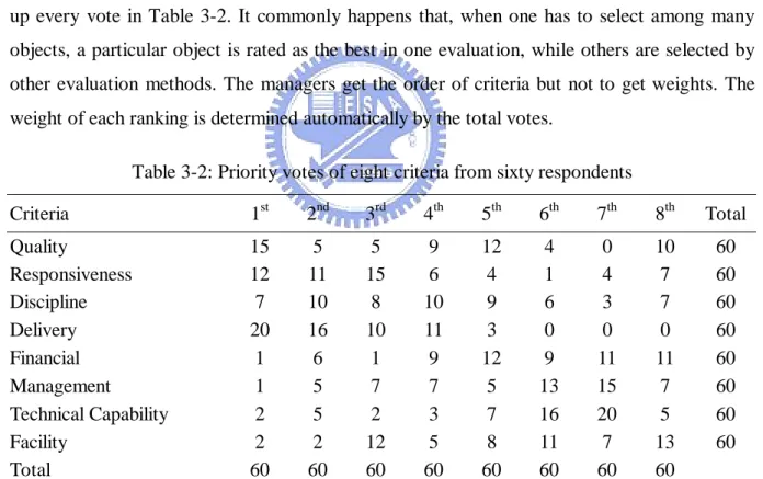
Table 3-2: Priority votes of eight criteria from sixty respondents ...29

Table 3-3: Priority votes and weights of thirteen sub-criteria ...30

Table 3-4: Supplier criteria score guideline ...32

Table 3-5: Rating of supplier-1 ...32

Table 3-6: Summary of the performance metrics...35

Table 3-7: Priority votes of seven criteria...37

Table 3-8: Priority votes and weights of eighteen sub-criteria ...37

Table 3-9: Priority votes and weights of three shipbuilding corporations ...38

Table 3-10: Rating of three shipbuilding corporations...40

Table 3-11: Rating of three shipbuilding corporations for seven criteria ...41

Table 3-12: Difference of the comparison between VAHP and AHP...42

Table 4-1: Rating scale of subjective indices...46

Table 4-2: The collected data of suppliers ...46

Table 4-3: The correspondence of DCU and DMU ...47

Table 4-4: Efficiency results ...48

Table 4-5: Efficient supplier composites ...48

Table 4-6: The composites data of two suppliers...49

NOTATIONS

MOBILP

K : the total number of activities.

m : the total number of resources.

s : the total number of products.

aik : the amounts of resource i consumed by activity k, i =1, … , m, and k =1, … , K.

crk : the amounts of product r produced by activity k, r =1, … , s, and k =1, … , K.

i

x′ : the objective function value of input i. r

y′ : the objective function value of output r.

wk : binary variable; wk=1 if kth activity is performed and wk=0 otherwise, k =1, … , K.

A : the m×K matrix of the m input value for the K activities. C : the s×K matrix of the s output value for the K activities.

Ω : the set of all possible DCUs.

ΩD : the set of DMUs that corresponding to DCUs in Ω.

DEA

DMUo : subscript “o” refers to the DMU currently under evaluation.

n : the total number of DMUs.

j : the index for DMUs, j =1, … , n.

i : the index for inputs, i =1, … , m.

r : the index for outputs, r =1, … , s.

xij : the units of input i consumed by DMUj, i = 1, … , m; j = 1, … , n.

yrj : the units of output r produced by DMUj, r = 1, … , s; j = 1, … , n.

xio : the units of input i consumed by DMUo (being evaluated), i = 1, … , m.

yro : the units of output r produced by DMUo (being evaluated), r = 1, … , s.

io

x′ : the units of input i consumed by DMUo (for efficient DMUs), i = 1, … , m.

ro

y′ : the units of output r produced by DMUo (for efficient DMUs) , r = 1, … , s.

µr : the weight assigned to output r, r =1, … , s.

νi : the weight assigned to input i, i =1, … , m.

λ_j : the variable for projecting DMUj, j =1, … , n.

+

r

s : the slack in the amount of output r, r =1, … , s.

−

i

s : the slack in the amount of input i, i =1, … , m. ε : the non-Archimedean (infinitesimal) constant.

ρ : the scalar number of input variable, ρ ≥ 1. ϖ : the scalar number of output variable, 0 <ϖ ≤ 1. θ, T, 'T , Z, 'Z , W, W : the objective values. '

δ, π, ψ, φ : the scalar variables.

θ*_{, δ}*_{, and π}* _{: the optimal values of θ, δ, and π, respectively.}

Vote-ranking method

g : the number of voters.

e : the number of places, e =1, … , E.

l : the number of criteria, l =1, … , L.

ule : the weights of the eth place with respect to the lth criterion.

xle : the total votes of the lth criterion for the eth place by g voters.

θll : the objective value.

d(e, ε) : the difference in weights between eth

place and (e+1)th place.

Criteria index

Dj : the planned delivery time for supplier j, j =1, … , n.

dj : the actual delivery time for supplier j, j =1, … , n.

C(Dj) : the penalty function of delivery time for supplier j, j =1, … , n.

Qj : the standard quality level for supplier j, j =1, … , n.

qj : the actual quality level for supplier j, j =1, … , n.

C(Qj) : the penalty function of quality for supplier j, j =1, … , n.

fj : the average scores of flexibility for supplier j, j =1, … , n.

cj : the average cost for supplier j, j =1, … , n.

1. INTRODUCTION

1.1 Introduction of Supply Chain

Under the high competitive and interrelated manufacturing environment of nowadays, an effective supplier selection process is very important for the success of any manufacturing organization. The emergence of a global competitive environment not only requires better use of supply chain (SC) resources to coordinate geographically dispersed manufacturing process and marketing activities but also has created a situation in which SC efficiency and effectiveness are critical to success. The suppliers of the supply chain perform interactively rather than independently, as the output of one organization could be the input of another organization. Selecting the right supplier is always a difficult task for top managers. Every decision needs to be affirmative and integrated by trading off performances of suppliers at each supply chain stage.

Fierce competition in today’s global markets, the introduction of products with short life cycles and the heightened expectations of customers have forced business enterprises to invest in and focus attention on their supply chains. In a typical supply, raw material is procured, items are produced in one or more factories, shipped to warehouse for intermediate storage, and then shipped to retailers or customers. The supply chain definition used in this research focus issue follows the spirit of the value chain concept: (Mabert & Venkataramanan, 1998)

Supply chain is the network of facilities and activities that performs the functions of product development, procurement of material from suppliers, the movement of materials between facilities, the manufacturing of products, the distribution of finished goods to customers and after-market support for sustainability.

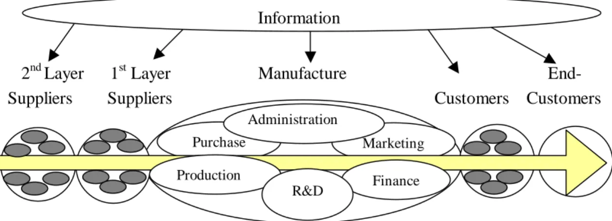
In order to survive and prosper, the companies should operate their supply chains as extended enterprises with relationship, which embrace business processes, from material extraction to consumption. The emergence of a global competitive environment not only has required better use of SC resources to coordinate geographically dispersed manufacturing and marketing activities but also has created a situation in which SC efficiency and effectiveness are critical to success. It depicts a simplified supply chain network structure, the information

and product flows and the key supply chain business processes penetrating functional silos within the company and various corporate silos across the supply chain in the Figure 1-1.

2nd Layer 1st Layer Manufacture End-

Suppliers Suppliers Customers Customers

Figure 1-1: Supply chain management

As this happens, supply chain takes on increased importance within the firm since costs, especially transportation, become a larger portion of the total cost structure. For example, if a firm seeks foreign suppliers for the materials entering its product or foreign locations to build its products, the motivation is to increase profit. A single firm is not generally able to control its entire product flow channel from the source of raw material to the points of final consumption. Therefore, ranking and selecting the right suppliers to organize a supply chain is very important but difficult tasks for managers. These issues are 1) the members of the supply chain, 2) the structural dimensions of the network, and 3) the different types of process links across the supply chain. Therefore, we will raise the following research topics when we construct the supply chain networks:

(1) Supply Chain Network Structure: which of them are the key supply chain members with the link processes?

(2) Supply Chain Business Process: what processes should be linked with these key supply chain members?

(3) Supply Chain Management Components: what level of integration should be applied for each process link?

Purchase Marketing Administration

Production _Finance

R&D

1.2 Problem Definition

In this dissertation, we are dealing with two issues of supplier selection in supply chain systems. The first issue is a group of decision-makers to rank the supplier candidates. We employ Analytic Hierarchy Process (AHP) for supplier selection. The pair-wise comparison method proposed by Saaty (1980) in AHP is substituted by a voting method. The voting method contains three steps. In the first step, each decision-maker ranks the alternatives to avoid the inconsistency that usually appeared in pair-wise comparison method. The second step is to summarize the votes each alternative earned in every rank. The third step is using a linear programming model to determine the weights assigned to every votes in those ranks. Then, the score each alternative earned is the sum of weighted votes.

The second issue is to select a set of multiple suppliers. There are 2K possible sets of multiple suppliers under selection if there are K supplier candidates. Cost, delivery, flexibility and quality are the four indices used to measure the suppliers’ performance. These four indices are also used to measure the performance of the possible sets under selection. The value of each index of a set is equal to the sum of values of the suppliers in it. We employ data envelopment analysis (DEA) to measure the relative performance of each set of multiple suppliers against the 2K possible sets with the four indices. Then, we perform sensitivity analysis on each index of candidates and provide different strategies in order to select various suppliers of a supply chain for customers.

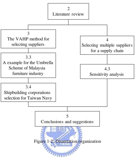
1.3 Dissertation Organization

Section two reviews the related literatures in supplier selection in supply chain, Multiple Criteria Decision-Making (MCDM), Multiple Objectives Binary Integer Linear Programming (MOBILP) and DEA. Section three presents the method to deal with the first issue. Section four illustrates the procedure for solving the addressed second issue. The structure of this study is illustrated in Figure 1-2.

2

Literature review

3

The VAHP method for selecting suppliers

3.3

A example for the Umbrella Scheme of Malaysia

furniture industry

3.4

Shipbuilding corporations selection for Taiwan Navy

4

Selecting multiple suppliers for a supply chain

4.3

Sensitivity analysis

5

Conclusions and suggestions

2. LITERATURE REVIEW

2.1 Supplier Selection in Supply Chain

One major aspect of the purchasing function is the selection of supplier, which includes the acquisition of required material, services and equipment for all types of business enterprises. The first step in any supplier rating procedure is to establish criteria for supplier selection. Weber et al. (1991, 1993) review and classify various articles related to the selection of supplier and discusse the impact of just-in-time (JIT) manufacturing strategy on supplier selection. They use Dickson’s 23 criteria and indicate that net price, delivery and quality are discussed in 80%, 59% and 54% of the 74 articles respectively. Identifying these capabilities is difficult because many different criteria are involved of being good supplier, trust and coordination play a major role are very important in achieving price reductions, quality improvement, reduced production development time and flexibility (Maloni & Benton 1997; Monczka et al., 1998).

Fawcett et al. (1997) represent a measure of the firm’s logistics performance concerning key factors such as cost, quality, delivery, flexibility and innovation. This is not an easy decision because there are many different criteria for a good supplier. The criteria to develop a partnership with a supply chain member organization are typically driven by the expectation of cost efficiency, delivery dependability, volume flexibility, information, quality and customer service (Choi et al., 1996; Motwani et al., 1998; Olhager & Selldin, 2004). Different companies have different specific requirements concerning supplier evaluation. For instance, in the automotive industry (Europe), functions of supplier logistics performance measurement include strategy formulation and clarification, management information, communication, motivation of suppliers, coordination and alignment (Schmitz & Platts, 2004). Different companies have different specific requirements concerning supplier evaluation. In Consumer Electronics Division of Philips Electronics Industries (Taiwan) Limited requirements for supplier selection include cost, delivery, flexibility, quality and response (Li et al., 1997).

Prahinski and Benton (2004) use structural equation modeling and collect data from 139 first-tier North American automotive suppliers. They indicate that when a purchaser utilizes collaborative communication, the supplier perceives a positive influence on the buy-supplier relationship. Hai (2004) adopts DEA model to evaluate the operational

efficiency of the top 57 semi-conduction companies in Taiwan and uses sensitivity analysis to examine the range of reliability of the best-practice frontier. Liu and Hai (2006a) use DEA to measure the efficiency of the possible suppliers. Each supplier is evaluated in four indices: cost, delivery, flexibility and quality. The problem is modeled as a MOBILP. We perform sensitivity analysis through perturbing the evaluation indices of each supplier. Narasimhan et al. (2001) propose a methodology for effective supplier performance evaluation based on DEA, a multi-factor productivity analysis technique. This article aids in supplier process improvement, which in turn enhances firm performance, allows for optimal allocation of resources for supplier development programs, and assists managers in restructuring their supply chain network (Ross & Droge, 2004).

Some authors apply an Activity Based Costing (ABC) approach for supplier selection. Management experts consider the economic aspects of supplier evaluation, and focus on the direct costs (price) and indirect costs (quality) of materials supplied by suppliers (Tagaras & Lee, 1996). However, since suppliers in a supply chain perform interactively, some cost-based mathematical models in the literature appear insufficient for delineating such key supply chain characteristics as multiple objectives and responsive requirements (Schneeweiss, 1998; Li & O’Brien, 1999).

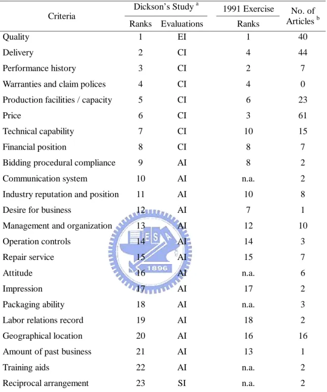
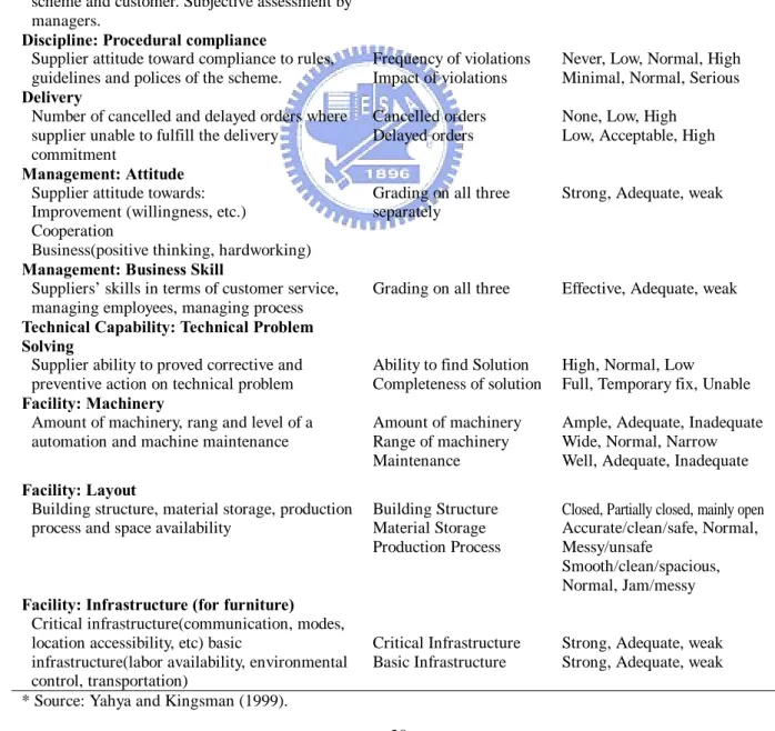
Dickson (1996) identifies 23 different criteria evaluated in the supplier selection process listed in Table 2-1. In that article, quality is treated as being of extreme importance while delivery, performance history, warranties and claim policies, production facilities and capacity, price, technical capability and financial position were viewed as being of considerable importance in the supplier selection process. Yahya and Kingsman (1999) operate the particular Umbrella Scheme of Malaysia’s furniture industry and use the criteria of supplier selection in Dickson’s research. A major part of the scheme is that all wooden furniture specified what kinds of requirements for government department and services, including school, administration, police, hospitals and military etc., are bought only from supplier companies that are members of the scheme.

Table 2-1: The different criteria evaluated in the supplier selection process Dickson’s Study a _{1991 Exercise} Criteria

Ranks Evaluations Ranks

No. of Articles b Quality

Delivery

Performance history

Warranties and claim polices Production facilities / capacity Price

Technical capability Financial position

Bidding procedural compliance Communication system

Industry reputation and position Desire for business

Management and organization Operation controls

Repair service Attitude Impression Packaging ability Labor relations record Geographical location Amount of past business Training aids Reciprocal arrangement 1 2 3 4 5 6 7 8 9 10 11 12 13 14 15 16 17 18 19 20 21 22 23 EI CI CI CI CI CI CI CI AI AI AI AI AI AI AI AI AI AI AI AI AI AI SI 1 4 2 4 6 3 10 8 8 n.a. 10 7 12 14 15 n.a. 17 n.a. 18 16 13 n.a. n.a. 40 44 7 0 23 61 15 7 2 2 8 1 10 3 7 6 2 3 2 16 1 2 2 a

EI= extreme important, CI= considerable important, AI= average important, SI= slight important.

b

No. of article in Weber, Current and Benton 1991 review of 74 papers. * Source: Yahya and Kingsman (1999).

The relationships with suppliers are different. They seem to work best when they are more family-like and less rational. Relationships with full commitment on all sides endure long enough to create value for the suppliers. In fact, the best organizational relationships, like the best marriage, are true partnerships that tend to meet certain criteria (Kanter, 1994):

Individual Excellence: Both partners are strong and have something of value to contribute to

the relationship. Their motives for entering into the relationship are positive.

Important: The relationship fits major strategic objectives of the partners, so they want to

make it work. Partners have long-term goals in which the relationship plays a key role.

Interdependence: The partners need each other. They have complementary assets and skills.

Neither can accomplish alone what both can together.

Investment: The partners invest to each other to demonstrate their respective stake in the

relationship of each other. They show tangible signs of long-term commitment by devoting financial and other resources to the relationship.

Information: Communication is reasonable open. Partners share information required to make

the relationship work, including their objectives and goals, technical data and knowledge of conflicts, trouble spots or changing situations.

Integration: The partners develop linkages and share the ways of operation so that they can

work together smoothly. They build broad connections between many people at many organizational levels. Partners become both teachers and learners.

Institutionalization: The relationship is given a formal status which clears responsibilities and

decision processes. It extends beyond the particular people who formed it, and it cannot be broken on a whim.

Integrity: The partners behave toward each other in honorable ways that justify and enhance

mutual trust. They do not abuse the information they gain, nor do they undermine each other.

2.2 Supply Chain Evaluation

Effective supply chain management envisioned as a solution to meet the constantly changing needs of the customer at low cost, high quality, short lead times and high variety. The motive behind the formation of supply chain arrangements is to increase channel competitiveness. Ahn and Lee (2004) propose an agent-based approach to improve the global efficiency of a supply chain by enabling participating companies to form a reasonably efficient supply chain dynamically and to minimize bullwhip effects in a supply chain via information sharing among cooperative agents. Talluri and Baker (2002) present a

multi-phase mathematical programming approach for effective supply chain network design. Their methodology develops a combination of multiple criteria efficiency models, based on game theory and concepts, and linear integer programming methods. Schneeweiss (2003) identifies different classes of distributed decision-making problems in supply chain management. These problem classes are developed in various sciences like applied mathematics, operations research, economics and artificial intelligence, particularly indicating possible synergies. They point to those distributed decision-making problems that have been proven to be of major relevance for supply chain management. Frohlich and Westbrook (2002) divide such integration into supply and demand integration. Supply integration includes delivery, evaluating supplier based on quality and delivery performance, establishing long-term contract with supplier and the elimination of paperwork. Demand integration includes increased access to demand information throughout the supply chain to permit rapid and efficient delivery, coordinated planning and improved logistics communication. Treville et al. (2004) propose a framework for prioritizing lead time reduction in a demand chain improvement project, using a typology of demand chains to identify and recommend trajectories to achieve desirable levels of market mediation performance.

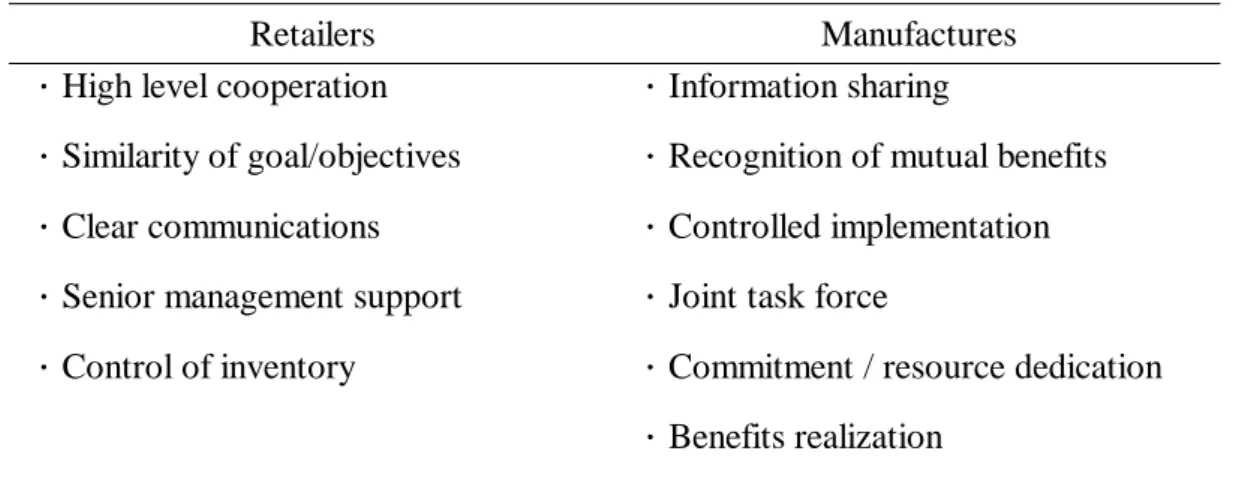
A question still remains outstanding is that what factors will result in successful supply chain relationships. It is also important to identify obstacles that that must be overcome to achieve success. The sidebar summarizes the findings of comprehensive research complete by Rosabeth Moss Kanter. Her study involves more than 500 interviews with managers from 37 firms in 11 different areas and countries that participate in collaborative arrangements. Table 2-2 and Table 2-3 summarize successful factors and common obstacles directly related to supply chain relationships. (Bowersox & Closs, 1996)

Table 2-2: Factors increasing likelihood of supply chain relationship success

Retailers Manufactures ．High level cooperation

．Similarity of goal/objectives ．Clear communications ．Senior management support ．Control of inventory

．Information sharing

．Recognition of mutual benefits ．Controlled implementation ．Joint task force

．Commitment / resource dedication ．Benefits realization

Table 2-3: Common obstacles confronted of supply chain relationships

Retailers Manufactures ．Low-volume stock keeping units

．Resistance of manufactures to change ．Information systems

．Non-compatible data formats

．Lack of communication ．Trust level

．Non-compatible systems

．Understanding of technical issues ．Resistance of customers to change ．Readiness of retailers

2.3 Multiple Criteria Methods for Evaluation

2.3.1 Multiple Criteria Decision-Making

In MCDM, it is assumed that there exist a number of alternatives for the decision-maker to decide, where each alternative is described by its performance on a number of criteria, attributes or objectives. Stewart (1996) defines a criterion that is a particular point of view according to which alternatives may be assessed and rank-ordered. An attribute is a particular feature of the alternative with which a numerical measure can be associated. An objective is a specific direction of preference defined in terms of attribute. The aim of MCDM is to provide support to the decision-maker in the process of making the choice between alternatives and may include the generation of a purposed “optimal” solution and/or some form of preference ranking.

The MCDM problems have two distinct categories: (1) multi-attribute decision analysis is most common applicable to problems with a small number of alternatives in an environment of uncertainty and (2) multiple criteria optimization are most common applied to deterministic problems in which the number of feasible alternative is large. The single objective mathematical programming problems are studied extensively in the past forty years. However, single objective decision-making methods reflect an earlier and simpler era. Almost every important real world problem involves more than one objective, and decision-makers find it imperative to evaluate solution alternatives according to multiple criteria. One may need to extend the single criterion problems to the multiple criteria problems.

Multiple criteria optimization is most commonly applied to deterministic problems, difficult public service policies and less controversial issues in business and government, e.g. nuclear power plant sitting, location of an airport and road construction, etc. The article is most fully covered by Keeney and Raiffa (1976) and Steuer (1986). The success of DEA in the area of performance evaluation together with the formal analogies existing between DEA and MCDM have leaded some authors to use DEA as a tool for MCDM (Doyle & Green; 1993, Stewart, 1994). The equivalence between the notion of “efficiency” in DEA and that of “convex efficiency” in MCDM is discussed in Belton and Vickers (1993) and Stewart (1996).

2.3.2 Multiple Objectives Binary Integer Linear Programming

Liu et al. (2000) and Liu and Lai (2000) first propose the problem defined as follows. Suppose there are K feasible activities, numbered k =1, … , K; each activity consumes varying amounts of m resources to produce s products. Specifically, activity k consumes amounts aik

of resource i, where i =1, … , m. Activity k produces crk of product r, where r =1, … , s. A

possible combination of the K feasible activities is denoted by w=(w1, w2, … , wK)

T

, which is called decision combination unit (DCU) throughout this paper. If the kth activity is performed, set wk=1, otherwise set wk=0. In total, there are 2

K

of possible DCUs. The traditional linear optimization technique solves the problem by formulating it as a MOBILP as following:

Objective function

Maximize yr = cr1w1 + … + crKwK, r = 1, … , s. (2-1)

Minimize xi = ai1w1 + … + aiKwK, i = 1, … , m.

Subject to wk∈B={0, 1}, k = 1, … , K.

In the practical situation, these constants are generally taken to be positive, aik >0 and

crk >0. The m×K matrix of input measures is denoted by A and the s×K matrix of output

measures is denoted by C. It can be expressed in matrix form: Maximize y=Cw

Minimize x=Aw Subject to w∈BK.

Instead of considering optimization of the criteria, they use DEA to develop the envelopment surface on the set of DMUs, Ω_D = {(x, y)| x=Aw, y=Cw, w∈Ω} to characterize efficiencies and inefficiencies where Ω is the set of all possible DCUs.

2.3.3 Data Envelopment Analysis

DEA is an analytical procedure developed for measuring the relative efficiency of DMUs that perform the same types of functions and have identical goals and objectives. Using DEA, the relative efficiency of DMUs that use multiple inputs to produce multiple outputs may be calculated. The weights used for each DMU are those which maximize the ratio between the weighted output and weighted input. DEA is a mathematical programming technique that calculates the relative efficiencies of n DMUs, based on multiple inputs and outputs. Given the data, we measured the efficiency of each DMU once and hence needed n optimizations, one for each DMU to be evaluated. Let the DMUj to be evaluated on any trial

be designated as DMU_o where o ranges from 1 to n. We solved the following fractional programming problem to obtain values for the input weight νi and output weight µr as

variables. 1 1 2 2 1 1 2 2 1 1 2 2 1 1 2 2 Max s.t. 1, 1, , ; 0, 1, , ; 0, 1, , . o o s so o o m mo j j s sj j j m mj i r y y y x x x y y y j n x x x i m r s µ µ µ θ ν ν ν µ µ µ ν ν ν ν µ + + + = + + + + + + ≤ = + + + ≥ = ≥ = K K K K K K K (2-2)

where xij = the units of input i consumed by DMUj, i = 1, … , m; j = 1, … , n.

y_rj = the units of output r produced by DMU_j, r = 1, … , s; j = 1, … , n. ν_i = the weight assigned to input i, i = 1, … , m.

µr = the weight assigned to output r, r = 1, … , s.

The constraints mean that the ratio of “virtual output” v.s. “virtual input” should not exceed 1 for every DMU. The objective is to obtain weights that maximized the ratio of

DMUo; the optimal objective value θ *

is at most 1. We convert this to managerial terms by assuming that all inputs and outputs have some nonzero worth; this is reflected in the weights ν_i and µ_r being assigned some positive value. Weber (1996) applies DEA to evaluate suppliers for an individual product and demonstrate its advantages for such a system. It is found that significant reduction in costs, late deliveries and rejected materials can be achieved if inefficient suppliers became DEA efficient.

DEA is based on mathematical programming and uses for characterizing efficiencies and inefficiencies of DMUs with the same multiple inputs and outputs. The two DEA models are going to be briefly reviewed (Charnes et al. 1991; Ali, 1997; Cooper et al., 2000).

(1) CCR Model

Let us assume that we have n DMUs using m inputs to secure s outputs. Let us denote

xij and yrj the level of the ith input and rth output respectively observed at DMUj. The technical

input model (2-3) first is developed by Charnes, Cooper and Rhodes (1978). They develop a classical model, referred as the CCR model. A nonlinear programming model provides a new definition of efficiency for use in evaluating activities of not-for-profit entities participating in public programs. The CCR model generalizes the single-output and single-input classical engineering-science ratio definition to multiple inputs and outputs without requiring pre-assigned weights.

CCR Model ⎯ Input Orientation Primal Form (CCRP-I)

1 1 1 1 Min s.t. , 1, , ; 0, 1, , ; 0, 1, , ; 0, 1, , ; 0, s m r i r i n j rj r ro j n io j ij i j j r i Z s s y s y r s x x s i m j n s r s s ψ ε ε λ ψ λ λ + − = = + = − = + − ′ = − − − = = − − = = ≥ = ≥ = ≥

∑

∑

∑

∑

K K K K 1, i= _K , m; (2-3) ψ : free in sign.

CCR Model ⎯ Input Orientation Dual Form (CCRD-I)

1 1 1 1 Max s.t. 1; 0, 1, , ; , 1, , ; , 1, , . s r ro r m i io i s m r rj i ij r i i r T y x y x j n i m r s µ ν µ ν ν ε µ ε = = = = ′ = = − ≤ = − ≤ − = − ≤ − =

∑

∑

∑

∑

K K K (2-4)

Several new constructs appear in this CCR model formulation. The variable “ε”, a non-Archimedean (infinitesimal) constant, appears both in the primal objective function and

as a lower bound for the multipliers in the dual problem. The scalar variable ψ*

is the proportional reduction applied to all inputs of DMU_o to improve efficiency. This reduction is applied simultaneously to all inputs and results in a radial movement toward the envelopment surface. The non-Archimedean ε in the primal objective function effectively allows the minimization over ψ*

to preempt the optimization involving the slacks. Thus, the optimization can be computed in a two-stage process with maximal reduction of inputs being achieved first, via the optimal ψ*

. Then, in the second stage, movement onto the efficient frontier is achieved via the slack variable. Evidently, the following two statements are equivalent:

(a) A DMU is efficient if and only if the following two conditions are satisfied. (a´) the optimal ψ*=1,

(b´) all slacks are zero.

(b) A DMU is efficient if and only if T′* =Z′* =1.

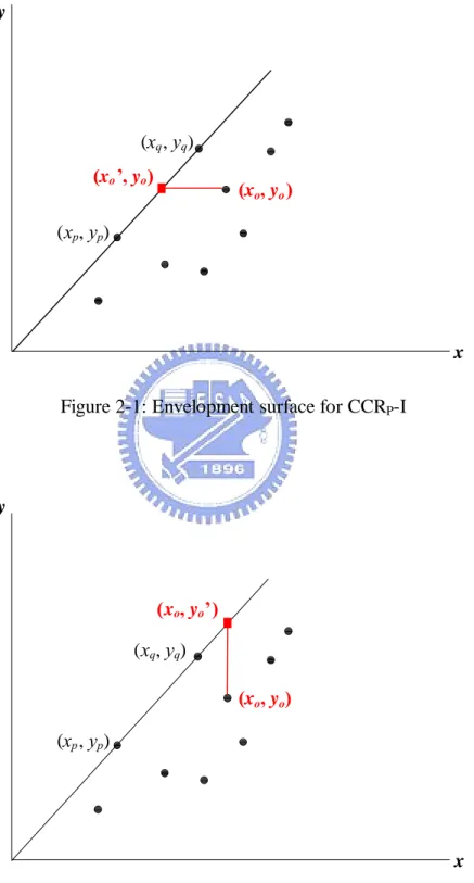
In an output orientated CCR model, the focus is shifted from input resource minimization to the output production maximization without exceeding the given levels. From the output orientated CCR model, maximal output augmentation is again accomplished through the variable φ applied to the output vector of DMUo.

CCR Model ⎯ Output Orientation Primal Form (CCRP-O)

1 1 1 1 Max s.t. , 1, , ; 0, 1, , ; 0, 1, , ; 0, 1, , ; 0, s m r i r i n j ij i io j n ro j rj r j j r i W s s x s x i m y y s r s j n s r s s φ ε ε λ φ λ λ + − = = − = + = + − ′ = + + + = = − + = = ≥ = ≥ = ≥

∑

∑

∑

∑

K K K K i=1, K , m; (2-5) φ: free in sign. If φ*

=1 and all input and output slacks are equal to zero, then DMU_o is efficient and is operating on the frontier; otherwise, if φ*

≠1 or (and) some input and (or) output slacks are nonzero, then DMUo is inefficient and could improve its efficiency by either reducing its

inputs or increasing its outputs over which management has control. A DMU is characterized as efficient in an input orientated CCR model if and only if it is characterized as efficient in the corresponding output orientated CCR model. The interpretation is similar to that applied

in the input orientation model mentioned above. We note in Figure 2-1 and Figure 2-2 that while the envelopment surfaces are identical for both the input and output orientations for the CCR model. An inefficient DMU is projected to different points on the envelopment surface.

x y (xq, yq) (xp, yp) (xo’, yo) (xo, yo)

Figure 2-1: Envelopment surface for CCRP-I

y x (xq, yq) (xp, yp) (xo, yo) (xo, yo’)

(2) BCC Model

Banker, Charnes and Cooper (1984) develop BCC model which separate the inefficiency into technical and scale inefficiencies. A separate variable is introduced which makes it possible to determine whether operations are conducted in regions of increasing, constant and decreasing return-to-scale in multiple inputs and outputs situations.

BCC model also admits both input and output orientations, and the formulation is similar to that for CCR model. The particular point of selected projection is dependent on the employed DEA model and the orientation. For instance, in an input orientated BCC model, one focuses on maximal movement toward the frontier through proportional reduction of inputs, whereas in an output orientation, one focuses on maximal movement via proportional augmentation of outputs. The input orientated BCC model evaluates the efficiency of DMUo

by solving the following linear program and the model is presented below: BCC Model ⎯ Input Orientation Primal Form (BCCP-I)

1 1 1 1 1 Min s.t. , 1, , ; 0, 1, , ; 1; 0, s m r i r i n j rj r ro j n io j ij i j n j j j Z s s y s y r s x x s i m δ ε ε λ δ λ λ λ + − = = + = − = = = − − − = = − − = = = ≥

∑

∑

∑

∑

∑

K K 1, , ; _r 0, 1, , ; _i 0, 1, , ; j₌ n s+_≥ r ₌ s s−_≥ i₌ m K K K (2-6) δ : free in sign.

BCC Model ⎯ Input Orientation Dual Form (BCCD-I)

0 1 1 0 1 1 0 Max s.t. 1; 0, 1, , ; , 1, , ; , 1, , ; : free in si s r ro r m i io i s m r rj i ij r i i r T y u x y x u j n i m r s u µ ν µ ν ν ε µ ε = = = = = − = − − ≤ = − ≤ − = − ≤ − =

∑

∑

∑

∑

K K K gn. (2-7)

In the dual linear programs for input orientated BCC model, we should note that neither the convexity constraint 1

1 =

∑

= n j j

λ nor the variable u0 appears in the formulation CCR

model. The absence of the convexity constraint enlarges the feasible region for CCR from the convex hull considered in BCCmodel to the conical hull of (or the convex cone generated by) DMUs.

As can be seen from the formulation below, the essential difference between the previous input and output orientated BCC model is that the Linear Programming (LP) now maximizes on π to achieve proportional output augmentation. One focuses on maximal movement via proportional augmentation of outputs. If a DMU is characterized as efficient in CCR model, it will also be characterized as efficient with BCC model. In particular, a DMU is characterized as efficient with an output orientation if and only if it is characterized as efficient with an input orientation applied to the same data. BCC model with an output orientation is presented below.

BCC Model ⎯ Output Orientation Primal Form (BCCP-O)

1 1 1 1 1 Max s.t. , 1, , ; 0, 1, , ; 1; 0, s m r i r i n j ij i io j n ro j rj r j n j j j W s s x s x i m y y s r s j π ε ε λ π λ λ λ + − = = − = + = = = + + + = = − + = = = ≥ =

∑

∑

∑

∑

∑

K K 1, _K , ; n s_r+≥0, r =1, _K , ; s s_i−≥0, i=1, _K , ;m (2-8) π : free in sign.

In an output orientation, the objective is to maximize output production while not exceeding the given resource levels. We again emphasize that this proportional output augmentation by itself may not be enough to achieve efficiency. Additional movement to the envelopment surface may be necessary and is accomplished via positive input and/or output slack values.

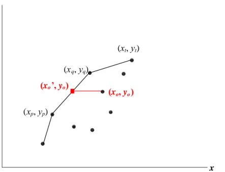
Finally, we should note in Figure 2-3 and Figure 2-4 that while the envelopment surfaces are identical for both the input and output orientations for BCC model. An inefficient DMU is projected to different points on the envelopment surface.

x y (xq, yq) (xp, yp) (xo’, yo) (xo, yo) (xt, yt)

Figure 2-3: Envelopment surface for BCCP-I

y x (xq, yq) (xp, yp) (xo, yo) (xt, yt) (xo, yo’)

Figure 2-4: Envelopment surface for BCCP-O

(3) Specifications of DEA

Two DEA models, BCC model and CCR model, are employed in this study. The first one is variable return-to-scale (VRS) model and the second one is the DEA constant return-to-scale (CRS) model. The essential difference between the VRS model and the CRS

model, input orientated model, is the addition of a new constraint 1 1 =

∑

= n j j

λ . With this added

constraint, the reference set is changed from the cone in the case of the CRS model to convex hull in the case of the VRS models. One result of this change is that the tested DMU is compared against a limited number of combinations. Banker and Thrall (1992) propose alternative method for determining return-to-scale in DEA. The methods for estimating return-to-scale in DEA are developed by Banker et al. (1984), Zhu and Shen (1995) and Banker et al. (1996).

CCR Return-To-Scale (RTS) Theorem (Banker and Thrall, 1992)

(a) If 1 1 * _>

∑

= n j j

λ in any alternate optima, then decreasing return-to-scale prevail.

(b) If 1 1 * =

∑

= n j j

λ in any alternate optima, then constant return-to-scale prevail.

(c) If 1 1 * <

∑

= n j j

λ in any alternate optima, then increasing return-to-scale prevail.

If we have a unique optimal solution in model (2-7), then CRS correspond to * 0

0 =

u ,

DRS correspond to * 0

0 >

u and IRS correspond to * 0

0 <

u considered over all alternate optima and when we are on the efficient production frontier.

To avoid the misclassification, we use the recent result to determine the RTS classification. We employ the output orientated CCR and BCC models to define a scale efficiency measure by _* 1 * = = π φ

τ . If τ =1, DMUo is called scale-efficient; otherwise, if τ >1 a

DMUo is called scale-inefficient. That is, let DMUo solution and λ be an optimal solution *j

associated with φ , then CRS prevail for DMU*

o if and only of φ =* π*, i.e., τ =1; otherwise,

if φ ≠* π*, i.e., τ >1 , then IRS prevail for DMUo if and only of 1

1 * <

∑

= n j j λ , and DRS prevail

for DMU_o if and only of 1

1 * >

∑

= n j j

λ . Using this method, one does not have to worry about

possible misclassification errors from multiple optimal solutions for *

j

λ , and the RTS classifications are readily obtained from the optimal solutions to the models (2-5) and (2-8).

The calculations of economies of scale have a direct interpretation in terms of the underlying dynamic evolution. A firm with decreasing return-to-scale has pushed its expansion too far, and management can be expected to consider the possibility of downsizing, laying off workers and reducing its scale of operations. Conversely, a firm with increasing return-to-scale will typically be engaged in rapid economic growth.

(4) Sensitivity analysis of DEA

Charnes et al. (1985) investigate the sensitivity of CCR model and Charnes and Neralic (1990) explore the sensitivity of the additive model in DEA. Zhu (1996) and Seiford and Zhu (1998) suggest a new approach to sensitivity analysis by using upward proportional variations of inputs and downward proportional variations of outputs on a modified CCR model. This results in sufficient conditions for the changes but does not alter the efficiency of DMUs. An efficient DMU is said to be robust to a given increase of an input, or a given decrease of an output, if the DMU remains efficient after the change.

, 1, 1, , . , 0 1, 1, , . io io ro ro x x i m y y r s ρ ρ ϖ ϖ ′ = ≥ = ⎧ ⎨ ′ = < ≤ = ⎩ K K (2-9)

In model (2-9), x_io and y_ro are the inputs and outputs of DMU_o. ρ and ϖ are the scalar numbers of input and output variables. It is assumed that inputs and outputs of remaining DMUs are unchanged.

3. THE VAHP METHOD FOR SELECTING SUPPLIERS

3.1 Introduction

Supplier selection has received extensive attention in supply chain management. Yahya and Kingsman (1999) integrate collaborative purchasing program where one of the aims is to select suppliers. They illustrate a new approach based on the use of Saaty’s AHP that is developed to assist in multiple criteria decision-making problems. In this section, we compare the appropriate total ranking sum of the selection number of rank vote to figure out the total weights of suppliers for selection, after determining the weights in a selected rank. This investigation presents a novel weighting procedure in replace of AHP’s paired comparison for selecting supplier. We provide a more simple method than AHP that is called Voting Analytic Hierarchy Process (VAHP), but not to lose the systematic approach of deriving the weights to be used and for scoring the performance of suppliers.

The AHP has found widespread application in decision-making problems, which involve multiple criteria in systems of many levels. The strongest features of the AHP are that they generate numerical priorities from the subjective knowledge expressed in the estimates of paired comparison matrices. The method is surely useful in evaluating suppliers’ weights in marketing or in ranking order, for instance. It is, however, difficult to determine suitable weight of each alternative in order. Noguchi et al. (2002) propose a new ordering to solve the weights of ranks by considering feasible solutions of the constraint set in linear program.

3.2 Related Theories and Models

3.2.1 Analytic Hierarchy Process

The multiple criteria aspects of decision analysis arise because outcomes must be evaluated in terms of several objectives. This is stated in terms of properties, either desirable or undesirable, that determine the decision-maker’s preference for the outcomes. The purpose of the value model is to take the various outcomes of the system models, determine the degree to which they satisfy each of the objectives, and then make the necessary trade-offs to achieve at a ranking for the alternatives that correctly expresses the preferences of the decision-maker. The AHP developed by Saaty (1980) is originally applied to uncertain decision problems with

multiple criteria, and has been widely used in solving problems of ranking, selection, optimization and prediction decisions. Generally, the AHP separates the complex decision problems into elements within a simplified hierarchical system. Through the pair-wise comparison of these principal eigenvector is then computed for the priority vector, which provides consistency measure of a decision-maker. The AHP methodology consists of the following four main steps:

(1) Develop the hierarchical structure (missions, criteria and alternatives). (2) Assign relative importance to each selection criterion of the mission. (3) Rank the alternatives under each criterion.

(4) Rank each alternative’s contributions to the mission.

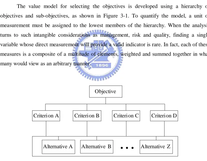
The value model for selecting the objectives is developed using a hierarchy of objectives and sub-objectives, as shown in Figure 3-1. To quantify the model, a unit of measurement must be assigned to the lowest members of the hierarchy. When the analysis turns to such intangible considerations as management, risk and quality, finding a single variable whose direct measurement will provide a valid indicator is rare. In fact, each of these measures is a composite of a multitude of elements, weighted and summed together in what many would view as an arbitrary manner.

Objective

Criterion A Criterion B Criterion C Criterion D

Alternative A Alternative B _{• • •} Alternative Z

Figure 3-1: Summary of three-level hierarchy for alternatives The seven pillars of the AHP are: (Saaty and Vargas, 2001)

(1) Ratio scale, proportionality and normalized ratio scales are central to the generation and synthesis of priorities, whether in the AHP or in any multiple criteria method

that needs to integrate existing ratio scale measurements with its own derived scales; in additional, ratio scales are the only way to generalize a decision theory to the case of dependence and feedback because ratio scales can be both multiplied and added – when they belong to the same scales such as a priority scale.

(2) Reciprocal paired comparison is used to express judgments semantically automatically linking them to a numerical fundamental scale of absolute numbers from which the principal eigenvector of priorities is then derived; the eigenvector shows the dominance of each element with respect to the other elements. The AHP has at least three modes to achieve the ranking of the alternatives: a) Relative, which ranks a few alternatives by comparing them in pairs and is particularly useful in new and exploratory decisions. b) Absolute, which rates an unlimited number of alternatives once at a time on intensity scales constructed separately for each coving criterion and is particularly useful in decisions where there is considerable knowledge to judge the relative importance of the intensities and develop priorities for them. c)

Benchmarking, which ranks alternatives by including a known alternative in the group and

comparing the other against it.

(3) Sensitivity of the principal right eigenvector to perturbation in judgments limits the number of elements in each set of comparisons to be few and requires that they be homogeneous.

(4) Homogeneous and clustering are used to extend the fundamental gradually from cluster to adjacent cluster, eventually enlarging the scale from 1-9 to 1-∞.

(5) Synthesis that can be extended to dependence and feedback is applied to the derived ratio scales to create a uni-dimensional ratio scale for representing the overall outcome. Synthesis of the scales derived in the decision structure can only be made to yield correct outcomes on known scales by additive weighting. It should be carefully noted that additive weighting in a hierarchical structure leads to a multi-linear form and hence is nonlinear.

(6) Rank preservation and reversal can be shown to occur without adding or deleting criteria, such as by simply introducing enough copies of an alternative or for other reasons; it follows that any decision theory must have at least two modes of synthesis.

(7) Group judgment must be integrated once at a time carefully and mathematically, taking into consideration when desired the experience, knowledge and power of each person involved in the decision, without the need to force consensus, or to use majority or other

ordinal ways of voting. The theorem regarding the impossibility of constructing a social utility function from individual utilities that satisfies four reasonable conditions, which found their validity with ordinal preferences, is no longer true when the preferences of cardinal ratio scale are used as in the AHP.

The strength of AHP lies in its ability to structure a complex, multi-person, multi-attribute problem hierarchically, and then to separately investigate each level of the hierarchy, combining results as the analysis progresses. Pair-wise comparison of the factors is undertaken, using a scale indicating the strength for which one higher-level factor dominates a lower-level factor. This scaling process can then be translated into priority weights or scores for ranking the alternatives. An integrated AHP and preemptive goal programming based multiple criteria decision-making methodology is developed to take into account both qualitative and quantitative factors in supplier selection (Partovi et al., 1990; Wang et al., 2004). AHP has been successfully applied in many situations and is designed for multiple criteria decisions, such as allocating order quantities for inventory (Partovi & Hopton, 1994), gauging organization performance (Lee et al., 1995; Rangon, 1996), weapon systems (Cheng, 1996), antivirus software (Mamaghani, 2002), total quality management (Dalu & Deshmukh, 2002), mutual funds (Saraoglu & Detzler, 2002) and project risk management (Dey, 2002).

3.2.2 Vote-Ranking Method

As for ranking of alternatives, one of the most familiar methods is to compare the weighted sum of their votes after the suitable weights of each alternatives has been determined. Cook and Kress (1990) present a procedure by applying data envelopment analysis to the problem of rank ordering the candidates in a preferential election. In such an election, each voter selects a subset of the candidates and places them in rank order; the poll organizer then establishes for each candidate a standing of the number of first, second, third place votes etc. received. And then, Green et al. (1996) develop it by setting specific constraints to weights. In what follow, this procedure is known as the “Green’s method”, which consists of the following two methods to set constraints: (1) the difference of weights between eth place and (e+1)th place for any e is allowed to be zero; (2) the above difference of weight must be strictly larger then zero.

Let us assume that there are more than one, say L (number) criteria for ranking. Next, let g be the number of voters, and E be the number of places. u_le denotes the weight of the eth place with respect to the lth criterion. Every candidate wishes to assign each weight ule in order

to maximize the weighted sum of votes to the lth criterion that is the score θll becomes the

largest. The “Green’s weak ordering” is defined as follows:

1 1 , 1 1 2 Max s.t. 1, 1, , ; ( 1, ) 0, 2, , ; 0. E ll le le e E le pe e l e le l l lE u x u x p L u u d e e E u u u θ ε ε = = − = ≤ = − ≥ − = ≥ = ≥ ≥ ≥ ≥

∑

∑

K K K (3-1)

The “Green’s strong ordering” is defined as follows:

1 1 , 1 1 2 Max s.t. 1, 1, , ; ( , ) 0, 1, , 1; 0. E ll le le e E le pe e le l e l l lE u x u x p L u u d e e E u u u θ ε ε = = + = ≤ = − ≥ = > = − ≥ ≥ ≥ ≥

∑

∑

K K K (3-2)

Here, xle are the total votes of the lth criterion for the eth place by g voters. We will

obtain some number xl1 of votes as first place, xl2 as second place, … , xle as e th

place, l =1, … ,

L, and e =1, … , E. d(e, ε)=ε appearing in model (3-2) constraint stands for the difference in

weights between eth place and (e+1)th place.

The above-mentioned Green’s method, however, has the following shortcoming: (a) application to concrete examples and (b) the change of ε influence the total ranking of objects. Especially, they do not examine (b) at all. The influence of ε can be analyzed by considering the feasible region of solutions (weights) obtained by LP, which is affected by the number of votes to the objects.

Noguchi et al. (2002) examine the application of Green’s method and showed different weights among objects to different results of ranking. Moreover, we do not only apply Noguchi’s strong ordering to a single–purpose problem, but also multi-purposes problem such as the supplier selection problem in a business corporation. In the total ranking method, one wants to set weights a particular constraint, “strong ordering” can be employed, which is characterized by the following constraint:

(a´) ) 1 ( 2 ) 2 1 ( 1 + = + + + = ≥ E gE E g u_le K ε , and

(b´) u_l1 ≥2u_l2 ≥3u_l3 ≥K≥Eu_lE.

Now we explain about the inequalities (a´). First of all, ule should be positive in order

not to lose information about the last place. We add the constraint ule ≥ ε > 0. The difference

in weights between (e−1)th

and eth place should be changed step by step to the last place. These weights should satisfy following inequalities:

0 ) ( ) ( ) (u_l1−u_l2 >_K> u_l,e−1−u_le >_K> u_l,E−1−u_lE > . Then, since _{, 1 , 1} 1 2 + + ₋ − − < − _{le le l e} le u e e u u

u , in order to make the weight of “strong

ordering”, replace > by ≥, i.e., we set

, 1 , 1 , 1 , 1 , 1 , 1 2 1 2 2 (since ) 1 1 ( 1) l e le le l e l e le le le l e l e le l e le e u u u u e e u u u u u e e u u e e u eu − + − + − − − − ≥ − − − ⇒ ≥ − ≥ − ⇒ ≥ − ⇒ − ≥

The value of ε is adjusted by both the number of votes and place. Consequently, we derive inequalities (a´) from the value of ε and inequalities (b´). In this multiple criteria case, the “Noguchi’s strong vote-ranking” is defined as follows:

1 1 , 1 Max s.t. 1, 1, , ; ( 1) , 1, , 1; 2 . ( 1) E ll le le e E le pe e le l e lE u x u x p L e u e u e E u gE E θ ε = = + = ≤ = ≥ + = − ≥ = +

∑

∑

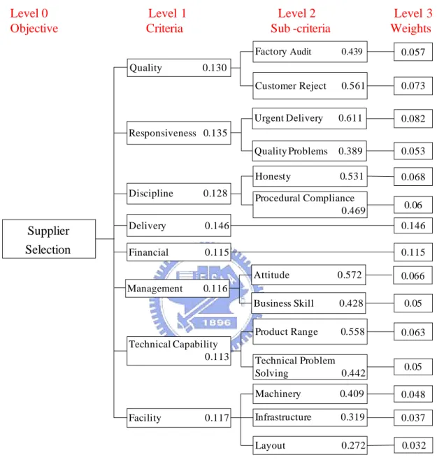
K K (3-3)

3.3 A Example for Umbrella Scheme of Malaysia’s Furniture Industry

Liu and Hai (2005a, 2005c) propose six steps procedure for assessing and selecting suppliers with numerical example for the Umbrella Scheme of Malaysia’s furniture industry that is from the paper of Yahya and Kingsman (1999). The problem is to select one of ten suppliers. The first step is structuring the problem into a hierarchy (see Figure 3-2). We set the objective for selecting suppliers on the top level. On the first level is that eight criteria