股票市場與外匯市場的連動性 - 政大學術集成

全文

(1) . 國立政治大學國際經營與貿易學系碩士論文 . 指導教授: 謝淑貞博士 . 立. 政治大 . ‧ 國. 學. . ‧. 股票市場與外匯市場的連動性. y. Nat. er. io. sit. Stock Prices and Exchange Rates: Evidences from. n. Emerging Markets and G-7 a v. i l C n h e n g c h i U . 研究生: 朱柏誠. 撰. 中華民國九十九年六月. .

(2) 謝辭從來沒料到自己竟然有機會在六月初就可以下筆撰寫謝辭。上學期在荷蘭當了一個很稱職的交換學生，一有機會就到歐洲各地遊山玩水，體驗了歐洲現代與傳統的文化也親眼見到了許多偉大的歷史古蹟以及名勝建築。在享受那樣愜意的生活同時，心中也暗忖回台後勢必得比同學更加努力方能如期畢業。回國後，轉眼間已經過了四個月，這期間順利的完成了碩士論文、碩士論文口試以及十七學分的期中考和期中報告，能熬過來最要感謝的莫過於謝淑貞謝老師，在撰寫論文時為我指明研究方向，在遇到困難時給我許多幫助和鼓勵，也謝謝老. 政治大做更深入的探究，還要感謝老師和我們這些尚未踏入社會的學生們分享寶貴的人立. 師體諒我有時無法如期交稿以及因為時間和能力的限制，沒辦法再針對研究主題. ‧ 國. 學. 生經驗和生活哲學並給予我們諸多建議，學生著實受益良多。亦要感謝口試委員謝德宗老師與葉小蓁老師在論文內容上給予我寶貴的意見。. ‧. 另外要感謝國貿所同學們的關心、鼓勵及幫助。同門師姐經艷、宛瑩和佳莉，謝. sit. y. Nat. 謝你們時常提醒我與老師 meeting 的時間、一起討論論文問題並互相打氣、邀請. al. er. io. 口試委員、佈置口試會場、準備茶點等，祝你們能順利找到心目中理想的工作。. v. n. 還要謝謝孟溢、冠呈、子誠、虹均、宗穎與順延這群國貿所的好哥兒們，提供我. Ch. engchi. i n U. 程式軟體並且熱心地解答我的許多疑問，也感謝你們在這段辛苦的期間陪我聊天、吃飯、打球，和你們相處帶給我很多的樂趣，為我紓解不少壓力。感謝所有陪伴我的同窗好友。最後要感謝一路上默默支持我的父母親和家人，由於你們的體諒與鼓勵使我在學業上沒有後顧之憂，你們對我的疼愛以及所付出的辛苦是我完成這篇論文最大的動力，願將此論文獻給我最愛的家人們，謝謝你們。. 柏誠謹 2010 年 06 月於政大 ii .

(3) 摘要本篇論文使用 Correlation of Coefficient 與 Johansen cointegration test 來探討股票市場與匯率市場之間的連動性。實證結果顯示股票市場與匯率市場之間有高度的相關性，特別是在西元 2000 年之後，全球呈現出集體的連動性。而此兩變數之間的關係亦可在不同的地區或是不同的工業化程度國家下看見不同的結果，歐體以及諸多新興市場等區域內皆呈現出股市與匯市相關係數的一致性。然而，當此研究以 Johansen cointegration test 來分析時，無法在此兩研究變數間發現顯著的長期關係。. 政治大. 關鍵字: Correlation of Coefficient、Johansen cointegration test、Stock prices、. 立. Exchange Rates. ‧. ‧ 國. 學. n. er. io. sit. y. Nat. al. Ch. engchi. iii . i n U. v.

(4) Abstract This study utilized Correlation of Coefficient as well as Johansen cointegration test to investigate the relationship between stock prices and exchange markets. The empirical results show that the two markets of study are highly correlated, especially after the year of 2000. Since then, the stock prices and exchange rates worldwide have presented one common trend, either negative correlation or positive. Different region, such as European Union or East Asian countries exclude Japan, and different level of industrialization lead to diverse relationship between exchange rates and stock prices.. 政治大 by using Johansen cointegration test. 立. Put this relationship in a long-term scope, however, no distinct trend can be discerned. Key words: Correlation of Coefficient、Johansen cointegration test、Stock prices、. ‧ 國. 學. Exchange Rates. ‧. n. er. io. sit. y. Nat. al. Ch. engchi. iv . i n U. v.

(5) Table of Contents 1. Introduction ................................................................................................................ 1 2. Literature Review ....................................................................................................... 4 3. Data and Methodology ............................................................................................. 10 3.1 Data Description ............................................................................................ 10 3.2 Methodology .................................................................................................. 15 3.2.1 Unit-root tests:The ADF test and PP test ............................................ 16 . 政治大 3.2.3. Johansen cointegration test ................................................................ 17 立 3.2.2. Coefficient of Correlation .................................................................. 17 . ‧ 國. 學. 4. Empirical Results ..................................................................................................... 19 4.1 Unit-root tests................................................................................................. 19 . ‧. 4.2 Coefficient of Correlation .............................................................................. 22 . sit. y. Nat. 4.3 Johansen cointegration test ............................................................................ 30 . io. al. er. 5. Conclusions .............................................................................................................. 32 . n. References .................................................................................................................... 33 . Ch. engchi. . i n U. v.

(6) List of Tables Table 4-1: Unit-root Tests at Level........................................................................ 20 Table 4-2: Unit-root Tests at First Differences ..................................................... 21 Table 4-3: Correlation Coefficients of Stock Prices and Exchange Rates ............ 25 Table 4-4: Correlation Coefficient (Entire Sample Period) .................................. 26 Table 4-5: Johansen Cointegration Test (Trace Test Statistics) ............................. 31 . 立. 政治大 Index of Figures. ‧ 國. 學. Figure 3-1: Stock Prices and Exchange Rates ....................................................... 12 . ‧. Figure 4-1: Coefficients of Correlation and Average Stock Prices ....................... 27 . n. er. io. sit. y. Nat. al. Ch. engchi. . i n U. v.

(7) . 1. Introduction Mutual relations between stock prices and exchange rates have attracted much attention of researchers and academics since the beginning of 1990s. Since the last quarter of last century, the world has witnessed significant changes in the international financial system such as the emergence of new capital markets, gradual abolishment of capital inflow barriers and foreign exchange restrictions, or the adoption of more flexible exchange rate arrangements in emerging countries. All the mentioned characteristics have broadened the variety of investment opportunities but, on the. 政治大. other hand, they have also increased the volatility of exchange rates and added a. 立. substantial portion of risk to the overall investment decision and portfolio. ‧ 國. 學. diversification process. Researching on the interaction between stock markets and exchange rates has therefore become more complex and has received more study. ‧. interest than before.. y. Nat. sit. Most of the early empirical literature that has examined the stock prices and. n. al. er. io. exchange rates relationship has focused on examining this relationship for the. i n U. v. developed countries, such as G-7. The focus has not been drawn to emerging. Ch. engchi. countries until 1997 Asian Financial Crisis. The results of these studies are, however, inconclusive. Some studies have found a significant positive relationship between stock prices and exchange rates [for instance, Aggarwal (1981)], while others have reported a significant negative relationship between the two [Ajayi and Mougoue (1996)]. On the other hand, there are some studies that have very weak or no association between the two [Bartov and Bodnor (1994)]. This paper is primarily motivated by several reasons. Firstly, prior studies only focus on either industrialized countries or emerging countries. Hardly have any study focused on both of them. With a larger sample countries including industrialized 1 .

(8) . countries and emerging countries, the mutual relation between stock markets and exchange rates in these countries can be reevaluated. Secondly, unlike developed countries, most developing countries do not adopt a freely floating exchange rate system and have more capital controls. 7(i.e., G-7) out of the 15 economies in this study follows a freely floating exchange rate arrangement. Examining these developed and developing economies enables us to discern the impact of different exchange rate arrangement and degree of financial markets liberalization on the linkages between stock markets and exchange markets.. 政治大 prices and exchange rates are mixed. Many reasons cause the mixed differences, 立 Thirdly, the results of past literatures studying relationship between the stock. involving the selection of the data sample—different countries and different period,. ‧ 國. 學. the methodology employed in the study. Therefore, this research covers more sample. ‧. countries with different degree of industrialization as well as a long-term timeframe to. y. Nat. detect an overall relationship between the two variables for the past decade.. er. io. sit. This research employs 7 developed countries (i.e., G-7), four Asian newly-developed countries—Taiwan, Hong Kong, Singapore and Korea, and BRIC. n. al. (i.e., Brazil, Russia, India. v i n C and China). In this h e n g c h i U study,. we view the four. newly-developed Asian countries as emerging countries as well. Our sample period includes 15-year data starting from 1995 to 2009. This period covers two to three business cycles, that is, bull market or bear market.. By studying the 15 developed. and developing countries in the scope of 15 years, we are able to see a broader observation of the relationship between stock markets and exchange rates geographically and chronologically. Our empirical results show a significant relationship between the two said variables in terms of the country as well as the time. Geographically, there is evidence suggesting that emerging countries possess negative relationship but not all emerging 2 .

(9) . countries do. Taiwan, Singapore, Korea, Brazil, Russia and India are the countries showing more negative relationships. In addition, countries within the same region tend to share a common trend. European countries—Germany, UK, France and Italy, for instance, show the same direction in the relationship for 9 years out of 11 years. Chronologically, 10 countries out of the 15 countries show a negative relationship between stock prices and exchange rates over the entire sample period. Moreover, since 2002, the beginning of another bull market, tendency of the relationship has become more consistent worldwide and the degree of relationship has also become. 政治大 The rest of this paper is organized as follows. Section 2 explains methodological 立. stronger globally.. .. issues. It discusses the theoretical links between the stock and foreign exchange. ‧ 國. 學. markets by calculating coefficients of correlation and employing Johansen. ‧. cointegration test. Section 3 presents the empirical results. Section 4 summarizes the. n. al. er. io. sit. y. Nat. main findings and gives the implications of these findings.. Ch. engchi. 3 . i n U. v.

(10) . 2. Literature Review In the existing literature in finance, the dynamic relationship between stock prices and exchange rates has drawn much attention from financial economists and practitioners since these two macroeconomics variables have influential impact on portfolio combinations for investors in financial markets. Most of the empirical literature examining the stock prices-exchange rates relationship focuses on examining this relationship for developed countries. In the past decade, however, more and more studies have studied this relationship based upon developed and. 政治大 Classical economic theory 立 suggests a relationship between the stock market. emerging markets.. ‧ 國. 學. performance and the exchange rate behavior. For instance, Dornbusch and Fischer (1980) put forward the “flow-oriented” model which suggests that changes in. ‧. exchange rates affect international competitiveness and trade balances, thereby. sit. y. Nat. influencing real income and output. Stock prices, generally interpreted as the present. al. er. io. values of future cash flows of firms, react to exchange rates changes and form the link. v. n. among future income, interest rate innovations, and current investment and. Ch. engchi. i n U. consumption decisions. Contrary to the “flow-oriented” model, Branson (1983) and Frankel (1983) put forward “stock-oriented” models of exchange rates. These models view exchange rates as equating the supply and demand for assets such as stocks and bonds. This approach gives the capital account an important role in determining exchange rate dynamics. Frank and Young (1972) are the first investigation that examines the relationship between the stock prices and exchange rates. They use six different exchange rates and find no significant relationship between these two variables. Employing monthly data, Aggarwal (1981) examines the relationship between US stock market indexes 4 .

(11) . and a trade-weighted value of the dollar for the period 1974-1978. He finds that the stock prices and exchange rates are positively correlated. In contrast, Soenen and Hanniger (1988) employ monthly data on stock prices and effective exchange rates for the period 1980-1986. They discover a strong negative relationship between the value of the US dollar and the change in stock prices. However, when they analyze the above relationship for a different period, they find a statistical significant negative impact of revaluation on stock prices. Solnik (1987) examines the impact of several variables (exchange rates, interest. 政治大 from 9 countries, including US, Japan, Germany, UK, France, Canada, Netherlands, 立 rates and changes in inflationary expectation) on stock prices. He uses monthly data. Belgium and Switzerland. He finds depreciation to have a positive but insignificant. ‧ 國. 學. influence on the US stock market compared to change in inflationary expectation and. ‧. interest rate. Ma and Kao (1990) provide some insights into probable reasons for the. y. Nat. different correlations between stock prices and exchange rates. They include six. er. io. sit. industrial economies to investigate the impact of changes in currency values on stock prices. Their results suggest that for an export-dominant economy, currency. al. n. v i n C hon the stock market, appreciation has a negative impact while currency appreciation engchi U boosts the stock market for an import-dominant country. The above early empirical. studies have focused on the contemporaneous relation between stock returns and exchange rates. Empirical works from the early stage focus on the linkage between the returns in the stock and exchange markets and does not use the levels of the series. Such a limitation was due to econometric assumptions about insufficient stationarity of financial data series. Stationarity is strictly required in regression analysis to avoid spurious inferences. By differencing the variables some information regarding a possible linear combination between the levels of the variables may be lost. The use 5 .

(12) . of cointegration technique overcomes the problem of nonstationarity and allows an investigation of both the levels and differences of exchange rates and stock prices (Phylaktis and Ravazzolo, 2000).. Bahmani-Oskooee and Sohrabian (1992) are. among the first to use cointegration and Granger causality to explain the direction of mutual relationships between the two variables. They analyze the long-run relationship between stock prices and exchange rates using cointegration as well as the causal relationship between the two by using Granger causality test. They employ monthly data on S&P 500 index and effective exchange rate for the period 1973-1988.. 政治大 employs the Granger causality 立. They are unable to find any long-run relationship between these variables. Rittenberg (1993). tests to examine the. relationship between exchange rates changes and price level changes in Turkey. Since. ‧ 國. 學. causality tests are sensitive to lag selection, therefore he employs three different. ‧. specific methods for optimal lag selection. In all cases, he finds that causality runs. y. Nat. from price level change to exchange rate changes but there is no feedback causality. er. io. sit. from exchange rate to price level changes. Bartov and Bodnor (1994) conclude that contemporaneous changes in the dollar have little power in explaining abnormal stock. al. n. v i n returns. In addition, they find aClagged change in theUdollar is negatively associated hengchi with abnormal stock returns. The regression results show that a lagged change in the. dollar has explanatory power with respect to errors in analysts’ forecasts of quarterly earnings. Ajayi and Mougoue (1996) observe significant interactions in eight industrial economies during 1985-1991. More concretely, they reveal a negative short-run and positive long-run effect of increase in domestic stock prices on domestic exchange rates. However, domestic currency depreciation influences the stock market in a negative way in the short-run. Donnelly and Sheehy (1996) document a significant contemporaneous relation between exchange rate and the market value of large UK 6 .

(13) . exporters. They attribute the difference between their findings and those based on US firms to (1) the UK is a more open economy than the US and (2) their focus on export-intensive firms. Yu (1997) employs daily data on markets of Hong Kong, Tokyo and Singapore over the period from January 3, 1983 to June 14, 1994 and detects bidirectional relationship in Tokyo but no causation for the Singapore market. Abdalla and Murinde (1997) apply cointegration approach to examine the long-run relationship between stock prices and real effective exchange rates in four Asian countries—India, Korea,. 政治大 relationship for Pakistan and Korea but does find a long-run relationship for India and 立 Pakistan and Philippines, using data from 1985 to 1994. Their study finds no long-run. Philippines. Since a long-run association is found for India and Philippines, they use. ‧ 國. 學. an error correction modeling approach to examine the causality for these two. ‧. countries. The results show a unidirectional causality from exchange rate to stock. y. Nat. price for India but for Philippines the reverse causation from stock price to exchange. er. io. sit. rate is found. Wu (2000) explores the effects on Singapore stock prices of Singapore-dollar exchange rates. The cointegration analysis suggests that for most of. al. n. v i n C hboth the SingaporeUdollar appreciation against the the selected periods in the 1990s engchi. US dollar and Malaysian ringgit and depreciation against Japanese yen and. Indonesian rupiah have positive long-run effects on stock prices. The influence of exchange rates on stock prices increases in a chronological order in the 1990s. Phylaktis and Ravazzolo (2000) apply the cointegration methodology and multivariate Granger causality tests to a group of Pacific Basin countries over the period 1980 to 1998. Their evidence suggests that stock and foreign exchange markets are positively related and that the US stock market acts as a conduit for these links. And these links are not found to be determined by foreign exchange restrictions. The general increase in international trade and the resultant increase in economic 7 .

(14) . integration have also increased financial integration and reduced the benefit of international diversification. Muhammad and Rasheed (2003) use monthly data from four South Asian countries, Bangladesh, India, Pakistan and Sri Lanka, and employ cointegration and error correction modeling approach to examine whether stock prices and exchange rates are related and the direction of causation if they are related. Their results show no long-run and short-run associations between stock prices and exchange rates for India and Pakistan. And there seems to be a bidirectional long-run causality between. 政治大 explores the nature of. these variables for Bangladesh and Sri Lanka. Yang and Doong (2004). 立. the mean and volatility. transmission mechanism between stock and foreign exchange markets for the G-7. ‧ 國. 學. countries. Evidence shows that movements of stock prices will affect future exchange. ‧. rate movements, but changes in exchange rates have less direct impact on future. y. Nat. changes of stock prices. Stavarek (2004) investigates the nature of the causal. er. io. sit. relationships among sock prices and effective exchange rates in four old EU member countries (Austria, France, Germany and the UK), four new EU member countries. al. n. v i n C hand Slovakia), andUthe United States. The results (Czech Republic, Hungary, Poland engchi show much stronger relationship in countries with developed capital and foreign-exchange market (i.e., old EU member and the US). Pan, Fok and Liu (2007) examine the dynamic linkages between the foreign exchange and stock markets for seven East Asian countries. Their results show a significant causal relation from exchange rates to stock prices for Hong Kong, Japan, Malaysia, and Thailand before 1997 Asian Financial Crisis. They also find a causal relation from the equity market to the foreign exchange market for Hong Kong, Korea and Singapore. Baharom, Habibullah and Royfaizal (2008) investigate the relationship between stock price and exchange rate pre and post Asian Financial Crisis 8 .

(15) . (i.e., January 1988 to June 1997 and July 1998 to December 2006) for Malaysia. By employing Johansen cointegration test, they conclude that there is no evidence of long-run relationship between the two variables of interest in the pre-and post-crisis periods. This study mainly focuses on the long-term relationship between stock prices and exchange rates. Our findings are consistent with Soenen and Hanniger (1988), Ajayi and Mougoue (1996) and Wu (2000), but in contrast to Ma and Kao (1990). Such differences are probably due to the sample period and pattern of data (i.e., daily or monthly).. 立. 政治大. ‧. ‧ 國. 學. n. er. io. sit. y. Nat. al. Ch. engchi. 9 . i n U. v.

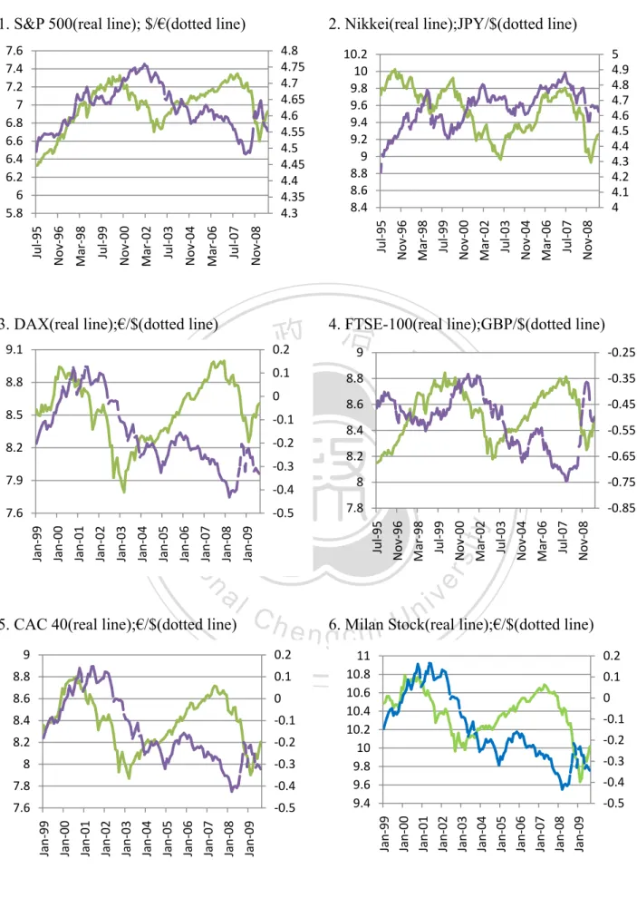
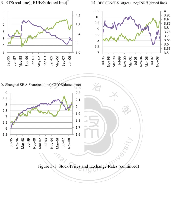
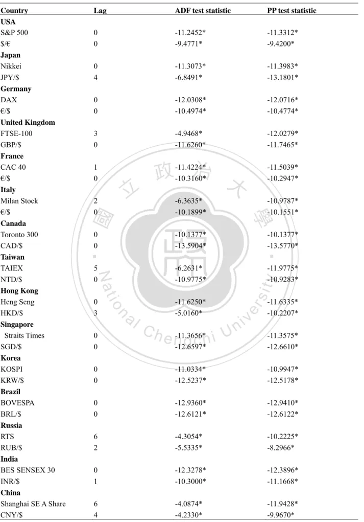
(16) . 3. Data and Methodology 3.1 Data Description Seven developed countries and eight emerging countries are selected for the empirical analysis. They include G-7, the United States of America, Japan, Germany, the United Kingdom, France, Italy and Canada; emerging countries include Taiwan, Hong Kong, Singapore, Korea, and BRIC—Brazil, Russia, India and China. The sample period varies for each country depending on the availability of data. For USA, Japan, UK, Canada, Taiwan, Hong Kong, Singapore, Korea, Brazil, India and China,. 政治大 to the launch of Euro in January of 1999, the sample starts from January 1999 to 立. the sample period is from May 1995 to August 2009. For Germany, France, Italy, due. August 2009. For Russia, the sample is from September 1995 to August 2009. The. ‧ 國. 學. data consists of monthly stock market index prices expressed in local currency, local. ‧. bilateral spot exchange rates prices expressed as domestic currency per U.S. dollar. y. Nat. (for US, Real Effective Exchange Rate based on CPI), and consumer price index. er. io. sit. (2005=100). All the observations are obtained from the International Financial Statistics Database and Browser, Datastream, and Taiwan Economic Journal and are. al. n. v i n end-of-the month observations. C All the series are expressed h e n g c h i U in logarithmic (LN) form.. The stock market index prices used are as follows: the S&P 500 for USA, Nikkei 225 for Japan, DAX for Germany, FTSE-100 for United Kingdom, CAC 40 for France, Milan Stock Index for Italy, Toronto 300 Composite for Canada, TAIEX for Taiwan, Heng Seng Price Index for Hong Kong, Singapore Strait Times Price Index for Singapore, KOSPI for Korea, BOVESPA for Brazil, RTS Index for Russia, BES SENSEX 30 Index for India and Shanghai SE A Share Index for China.. 10 .

(17) . The real exchange rate is defined as1 (1). , where. is the consumer price index for the countries,. exchange rate of each country and. is the consumer price index for US. For the. real exchange rate of US, the CPI of Germany is used.. 立. 政治大. ‧. ‧ 國. 學. n. er. io. sit. y. Nat. al. Ch. engchi. i n U.                                                         1. . is the nominal. The real exchange rate is defined by Phylaktis and Ravazzolo (2000) 11 . v.

(18) . 2. Nikkei(real line);JPY/$(dotted line) 4.8 4.75 4.7 4.65 4.6 4.55 4.5 4.45 4.4 4.35 4.3. ‐0.4. 7.6. ‐0.5. Nov‐08. Jul‐07. Mar‐06. Nov‐04. Jul‐03. Mar‐02. Nov‐00. Jul‐99. Nov‐08. Jul‐07. Mar‐06. Nov‐04. Jul‐03. y Mar‐02. sit. Nov‐00. Jul‐99. Mar‐98. 0 ‐0.1 ‐0.2 ‐0.3 ‐0.4 ‐0.5. Figure 3-1: Stock Prices and Exchange Rates 12 . 0.2 0.1. Jan‐99 Jan‐00 Jan‐01 Jan‐02 Jan‐03 Jan‐04 Jan‐05 Jan‐06 Jan‐07 Jan‐08 Jan‐09. 7.8 Jan‐08. ‐0.3. 11 10.8 10.6 10.4 10.2 10 9.8 9.6 9.4. Jan‐09. 8. Jan‐07. ‐0.2. Jan‐06. 8.2. Jan‐05. ‐0.1. Jan‐04. 8.4. Jan‐03. 0. Jan‐02. 8.6. Jan‐01. 0.1. Jan‐00. ‐0.85. er. n. 8.8. . ‐0.75. v i n Ch line);€/$(dotted line) U e n g6. cMilan h i Stock(real 0.2. Jan‐99. Mar‐98. Jul‐95 Jul‐95. Jan‐09. Jan‐08. io. Jan‐07. Jan‐04. Jan‐03. Jan‐02. Jan‐01. Jan‐00. Jan‐99. 7.8. ‐0.5. 9. ‐0.55 ‐0.65. 8. ‐0.4. 5. CAC 40(real line);€/$(dotted line). ‐0.45. 8.2. ‐0.3. al. 8.6 8.4. ‐0.2. Nat. 7.6. ‐0.1. ‐0.35. ‧. 7.9. Jan‐06. 8.2. Jan‐05. 8.5. 8.8. 學. ‧ 國. 0. Nov‐96. 立. 8.8. 5 4.9 4.8 4.7 4.6 4.5 4.4 4.3 4.2 4.1 4. 4. FTSE-100(real line);GBP/$(dotted line) 治9 政 0.2 ‐0.25 大 0.1. 3. DAX(real line);€/$(dotted line) 9.1. 10.2 10 9.8 9.6 9.4 9.2 9 8.8 8.6 8.4. Nov‐08. Jul‐07. Mar‐06. Nov‐04. Jul‐03. Mar‐02. Nov‐00. Jul‐99. Mar‐98. Nov‐96. Jul‐95. 7.6 7.4 7.2 7 6.8 6.6 6.4 6.2 6 5.8. Nov‐96. 1. S&P 500(real line); $/€(dotted line).

(19) . 7. Toronto 300(real line); CAD/$(dotted line) 0.5. 9.4. 3.7. 0.4. 9.2. 3.6. 9. 3.5. 8.8. 3.4. 8.6. 3.3. 8.4. 3.2. 8.2. 3.1. 0.3 0.2 0.1 0. 8 Nov‐08. Jul‐07. Mar‐06. Nov‐04. Jul‐03. Mar‐02. Nov‐00. Jul‐99. Mar‐98. 3 Jul‐95. Nov‐08. Jul‐07. Mar‐06. Jul‐03. Nov‐04. Mar‐02. Nov‐00. Jul‐99. Mar‐98. Jul‐95. Nov‐96. ‐0.1. Nov‐96. 9.8 9.6 9.4 9.2 9 8.8 8.6 8.4 8.2 8. 8. TAIEX(real line);NTD/$(dotted line). 10. Straits Times(real line);SGD/$(dotted line) 政治 8.4 0.6 大 2.1. 9. Heng Seng(real line);HKD/$(dotted line). 7.6. 0.1. io. Nov‐08. Jul‐07. Mar‐06. er. Nov‐04. 0. Jul‐03. y Mar‐02. 6.4. 0.3. sit. 1.6. Nov‐00. 6.8. Jul‐99. 1.7. 0.4. 0.2. Jul‐95. 7.2. Jul‐95 Nov‐96 Mar‐98 Jul‐99 Nov‐00 Mar‐02 Jul‐03 Nov‐04 Mar‐06 Jul‐07 Nov‐08. Nat. 1.8. Mar‐98. 1.9. ‧. ‧ 國. 0.5. 8. 2. Nov‐96. 立. 學. 10.5 10.3 10.1 9.9 9.7 9.5 9.3 9.1 8.9 8.7 8.5. al. n. v i n Ch 11. KOSPI (real line);KRW/$(dotted line) e n g12.cBOVESPA h i U (real line);BRL/$(dotted line). Figure 3-1: Stock Prices and Exchange Rates (continued) 13 . Nov‐08. Jul‐07. Mar‐06. Nov‐04. Jul‐03. Nov‐08. Jul‐07. Mar‐06. Nov‐04. 6.4 Jul‐03. 5.4 Mar‐02. 6.6 Nov‐00. 5.8 Jul‐99. 6.8. Mar‐98. 6.2. Nov‐96. 7. Jul‐95. 6.6. Mar‐02. 7.2. Nov‐00. 7. Jul‐99. 7.4. 1.8 1.6 1.4 1.2 1 0.8 0.6 0.4 0.2. Mar‐98. 7.4. 11.5 11 10.5 10 9.5 9 8.5 8 7.5 7. Nov‐96. 7.6. Jul‐95. 7.8.

(20) . 13. RTS(real line); RUB/$(dotted line)2. 14. BES SENSEX 30(real line);INR/$(dotted line) 10.5. 9 4.2. 8. 3.8. 7. 4 3.95 3.9 3.85 3.8 3.75 3.7 3.65 3.6 3.55 3.5. 10 9.5 9. 6. 3.4. 5 3. 4. 8 7.5 7 Jul‐95 Nov‐96 Mar‐98 Jul‐99 Nov‐00 Mar‐02 Jul‐03 Nov‐04 Mar‐06 Jul‐07 Nov‐08. Jan‐09. Sep‐07. May‐06. Jan‐05. Sep‐03. May‐02. Jan‐01. Sep‐99. Sep‐95. May‐98. 2.6 Jan‐97. 3. 8.5. 治政 2.2 大. 15. Shanghai SE A Share(real line);CNY/$(dotted line) 9. 立. 8.5. 2.1. 8. y. sit. io. al. Nov‐08. Jul‐07. 1.6. er. 1.7 Mar‐06. Nov‐00. Jul‐99. Mar‐98. Nov‐96. Jul‐95. 1.8. Nat. 5.5. Nov‐04. 6. 1.9. ‧. 6.5. Jul‐03. 7. Mar‐02. ‧ 國. 2. 學. 7.5. n. v i n Figure 3-1: StockC Prices Rates (continued) h eand n gExchange chi U.                                                        . 2. . Following the literature, all data series have been taken natural logarithms. 14 .

(21) . 3.2 Methodology Generally speaking, most of the time series variables possess the characteristic of nonstationarity. A time series variable is stationary under the condition that this variable’s mean, variance and function of autocorrelation will not vary in accordance with the change of the time. Such condition, however, will be violated by the fluctuations over time. If we employ the traditional econometric models and methods in dealing with time series data having the characteristic of nonstationarity, the residuals we get may be non-stationary due to the high autocorrelation within the. 政治大 help us understand the true relationship among the variables. Stock prices and 立. residuals. Then, we may end up producing one spurious regression which will not. exchange rates employed in this study are typically non-stationary. In order to cope. ‧ 國. 學. with non-stationary economic and financial time series analysis, Granger (1986),. ‧. Engle & Granger (1987) and Johansen (1988, 1991) put forward the cointegration test.. y. Nat. This model provides a solution to the problem of spurious regression.. er. io. sit. In the beginning, this research employs unit-root tests including Augmented Dickey-Fuller (ADF) test and Phillips-Perron (PP) test, and Johansen cointegration. al. n. v i n C hIn addition to these test as the primary methodologies. two tests, the correlation of engchi U. coefficients between stock prices and exchange rates will be calculated annually. By employing these methodologies, whether the long-term relationship exists between. stock prices and exchange markets in the countries of interest will be tested and observed. The process of this study begins with the unit-root tests on each country’s samples. After determining the time series order Ι (*), we proceed to Johansen cointegration test to determine the optimal cointegration vector. The methodologies are explained as follows:. 15 .

(22) . 3.2.1 Unit-root tests: The ADF test and PP test Granger and Newbold (1974) firstly point out that using non-stationary macroeconomic variables in time series analysis causes superiority problems in regression. The issue of unit-root of such variables is empirically demonstrated in Nelson and Plosser (1982) and since then this important property of macroeconomic and financial data series has been generally accepted. Many studies have lately shown that majority of time series variables are non-stationary or integrated of order 1. Thus, a unit-root test should precede any empirical study employing such variables. There. 政治大 principally Augmented Dickey-Fuller test and Phillips-Perron test have been widely 立. have been a variety of proposed methods for implementing stationarity test and. used in econometric data. Also this study, as a first step, executes both unit-root tests. ‧ 國. 學. to investigate whether the time series of stock prices and exchange rates are stationary. ‧. or not. ADF unit-root test (Dickey and Fuller 1979) is often used to determine the. n. al. where ∆. :. 0. :. 0. . i n U. v. (2). e n g c h i is the white noise.. is the first difference of variable X,. ADF test uses. If. Ch. sit. ∆. er. io. ∆. y. Nat. time series order Ι (*). Its unit-root test regression is:. to establish the null and alternative hypothesis:. is significant different from zero, null hypothesis will be rejected, which means. the variable does not have a unit-root. Although ADF test takes the problem of autocorrelation into consideration, the characteristic of homoscedasticity in time series exists. Phillips and Perron (1988) made a more relaxed assumption on the basis of ADF test and this leads to the 16 .

(23) . development of PP test. The test is robust with respect to unspecified autocorrelation and heteroscedasticity in the disturbance process of the test equation. 3.2.2. Coefficient of Correlation Correlation coefficient is a measure of the degree of association between two variables. Its definition is: ∑ ∑ ∑. ∑ ∑. (3) ∑. 政治大 . This is also known. 立. as sample correlation. ‧ 國. 學. coefficient.. ∑ ∑. ∑ ,. where. ∑. 3.2.3. Johansen cointegration test. ‧. According to the concept of cointegration, two or more non-stationary time. ~. ,. ,…,. follow:. ,…,. component. of. the. vector. v. are considered to be cointegrated of order d, b, denoted. Ch. i n U. e n g care h i stationary. if first, all the component. integrated of order d and noted as ,. the. sit. y. al. as. er. expressed. n. ,. is. io. framework. Nat. series share a common trend, then they are said to be cointegrated. The theoretical. ~. after n difference, or. ; second, presence of a vector. in such that linear combination. where the vector β in named the cointegrating vector. Some noteworthy characteristics of this model are that the cointegration relationship obtained indicates a linear combination of non-stationary variables, in which all variables must be integrated of the same order and moreover if there are n series of variables, there may be as many as n-1 linearly independent cointegrating vectors. Johansen’s (1991) cointegration test is adopted to determine whether the linear 17 .

(24) . combination of the series possesses a long-run equilibrium relationship. The numbers of significant cointegrating vectors in non-stationary time series are tested by using and λ. the maximum likelihood based on λ. introduced by Johansen and. Juselius (1990). The advantage of this test is that it utilizes test statistic that can be used to evaluate cointegration relationship among a group of two or more variables. Therefore, it is a superior test as it can deal with two or more variables that may be more than one cointegrating vector in the system. In the Johansen procedure, it involves the identification of rank of the n x n matrix Π in the specification given by:. 立. ∆. 政治大 ∆. (4). ‧ 國. 學. where Yt is a column vector of the n variables, Δ is the difference operator, Γ and Π. ‧. are the coefficient matrices, k denotes the lag length and δ is a constant. In the absence. sit. y. Nat. of cointegrating vector, Π is a singular matrix, which means that the cointegrating. io. er. vector rank is equal to zero. On the other hand, in a cointegrated scenario, the rank of Π could be anywhere between zero.. al. n. v i n C h test providesUa test for the rank of Π, namely The Johansen Maximum likelihood engchi. the trace test (λ (λ. ). The. ), on which this study focuses, and the maximum eigenvalue test statistic tests the null hypothesis that the number of distinct. cointegrating vectors is less than or equal to r against alternative hypothesis. The test statistic is given as follow: 1. (5). where p is the number of separate series to be analyzed, T is the number of usable observations and. is the estimated eigenvalues. 18 . .

(25) . 4. Empirical Results 4.1 Unit-root tests Before proceeding to the cointegration test, unit root tests are performed on each of the national stock indices and the exchange rate series to determine the order of cointegration of these series. We employed the Augmented Dickey-Fuller test3 and the Phillips-Perron test to conduct the unit root tests. The tests are performed for the entire sample on both the level and first difference of the stock indices and exchange rates series. Table 4-1 and Table 4-2 report the results of these tests.. 政治大 be rejected in the stock prices 立 and exchange rates of all countries in the study. This Table 4-1 reveals that the null hypothesis of a unit-root in the level series cannot. ‧ 國. 學. indicates that both the series are non-stationary in all countries. Table 4-2 reports that the null hypothesis of a unit-root in the first difference of stock prices and exchanges. ‧. series is rejected for all the countries. Therefore, all the series of USA, Japan,. sit. y. Nat. Germany, United Kingdom, France, Italy, Canada, Taiwan, Hong Kong, Korea,. al. er. io. Singapore, Brazil, Russia, India and China are integrated for order one, i.e., Ι(1). This. v. n. means we can apply cointegration test for these countries to examine the long-run. Ch. engchi. relationship between stock prices and exchange rates.. i n U.                                                         3. . The optimal lag length is selected based on Akaike’s information criterion (AIC). 19 .

(26) . Table 4-1: Unit-root Tests at Level Country. Lag. ADF test statistic. PP test statistic. USA S&P 500. 1. -2.7305. -2.6577. $/€. 1. -1.1861. -1.2390. Nikkei. 1. -1.5880. -1.6042. JPY/$. 0. -3.2491. -3.4064. DAX. 0. -2.1884. -2.2471. €/$. 1. -0.5684. -0.3465. FTSE-100. 4. -2.3634. -2.2868. GBP/$. 0. -1.5494. -1.8590. CAC 40. 1. -2.2677. -2.1918. €/$. 0. Japan. Germany. United Kingdom. France. Italy. 立. -2.0953. -1.8424. -0.6677. -0.7360. 7. -2.9127. NTD/$. 1. -1.8799. Heng Seng. Nat. 學. TAIEX. y. 0. 1. -2.0522. sit. 8. €/$. -0.8881. ‧ 國. Milan Stock. 政 -0.8280治大. HKD/$. 13. Toronto 300 CAD/$. Hong Kong. -2.0036. 0. -1.0321. 2. SGD/$. 0. -1.5969. n. Straits Times. io. Singapore. al. Ch. i U e n-2.1688 h c g -2.2608. -1.8450 -1.0925. ‧. Taiwan. 1. -2.7451. -2.2184. er. Canada. v ni. -1.8866 -0.1914 -1.9683 -2.2704. Korea KOSPI. 1. -1.4360. -1.2757. KRW/$. 0. -2.4031. -2.4547. BOVESPA. 0. -1.3362. -1.3499. BRL/$. 0. -1.5177. -1.5378. RTS. 7. -1.5904. -1.5374. RUB/$. 3. -1.2329. -0.9596. BES SENSEX 30. 0. -0.1983. -0.3629. INR/$. 2. -0.8266. -1.2259. Brazil. Russia. India. China Shanghai SE A Share. 7. -2.7423. -1.8854. CNY/$. 1. -2.4913. -3.0117. *and ** denote the rejection of unit-root hypothesis at 1% and 5% significance levels, respectively. 20 .

(27) . Table 4-2: Unit-root Tests at First Differences Lag. ADF test statistic. PP test statistic. 0 0. -11.2452* -9.4771*. -11.3312* -9.4200*. 0 4. -11.3073* -6.8491*. -11.3983* -13.1801*. 0 0. -12.0308* -10.4974*. -12.0716* -10.4774*. 3 0. -4.9468* -11.6260*. -12.0279* -11.7465*. 5 0. -6.2631* -10.9775*. 0 3. -11.6250* -5.0160*. io. n. 0 0. al. Ch. e n-11.3656* gchi -12.6597*. -10.1377* -13.5770*. -11.9775* -10.9283*. y. ‧ 國. -10.1377* -13.5904*. ‧. 0 0. -10.9787* -10.1551*. 學. -6.3635* -10.1899*. -11.5039* -10.2947*. sit. 立. 2 0. 治政 -11.4224* -10.3160* 大. er. 1 0. Nat. Country USA S&P 500 $/€ Japan Nikkei JPY/$ Germany DAX €/$ United Kingdom FTSE-100 GBP/$ France CAC 40 €/$ Italy Milan Stock €/$ Canada Toronto 300 CAD/$ Taiwan TAIEX NTD/$ Hong Kong Heng Seng HKD/$ Singapore Straits Times SGD/$ Korea KOSPI KRW/$ Brazil BOVESPA BRL/$ Russia RTS RUB/$ India BES SENSEX 30 INR/$ China Shanghai SE A Share CNY/$. i n U. v. -11.6335* -10.2207* -11.3575* -12.6610*. 0 0. -11.0334* -12.5237*. -10.9947* -12.5178*. 0 0. -12.9360* -12.6121*. -12.9410* -12.6122*. 6 2. -4.3054* -5.5335*. -10.2225* -8.2966*. 0 1. -12.3278* -10.3000*. -12.3896* -11.1668*. 6 4. -4.0874* -4.2330*. -11.9428* -9.9670*. *and ** denote the rejection of unit-root hypothesis at 1% and 5% significance levels, respectively.. 21 .

(28) . 4.2 Coefficient of Correlation Prior to testing for cointegration, the dynamic correlation coefficients for each country will be calculated and discussed. Coefficient of correlation measures the direction, i.e., negative, zero or positive and its magnitude of the two variable’s relationship in this study. From evidences in table 4-3, we can observe several characteristics of the relationship depending on the country and the time. First, we find substantial differences in the power of coefficients of correlation between two geographical areas. For G-7 countries, Japan, UK and Canada separately. 政治大 years. This indicates that when pound appreciates against US dollar and when 立 have 6 years, 8 years and 11 years of negative coefficient of correlation out of 15. Canadian dollar appreciates against US dollar, the domestic stock markets tend to rise. ‧ 國. 學. in these two countries. On the other hand, the stock markets tend to fall while. ‧. Japanese yen appreciates against US dollar. The number of negative coefficients. y. Nat. between US dollar and S&P 500 are 10. This means when US dollar appreciates, S&P. er. io. sit. 500 is likely to fall. For Eurozone countries, Germany, France and Italy each has 7 years, 5 years and 5 years of negative coefficient of correlation in 11 years, which. al. n. v i n C h the US dollar, German means when euro appreciates against stock market tends to rise engchi U but Italian and French stock markets tend to fall. We also can see the high unification of financial markets among the four European countries. The evidence is that 9 years out of the 11-year sample period from 1999 to 2009, these countries share the same trend in the relation of stock markets and exchange rates. Contrary to the inconsistent frequency of negative correlation coefficients among G-7 countries, the emerging countries appear to be more uniform. For Taiwan, Singapore, Korea, Brazil, Russia and India, it is 13 years, 13 years, 12 years, 12 years, 12 years and 9 years out of 15-year sample period. This signifies that when the currencies in these countries appreciate against US dollar, the stock markets tend to 22 .

(29) . rise. One of the main factors in explaining why the above countries have a uniform result is that the foreign capital plays an essential role in these countries’ stock markets. Thus, when the international capital flows into these countries for the purpose of investing in the stock markets, the exchange rates will appreciate in advance of the rise in stock markets. Secondly, concerning the time point of view, the first business cycle from 1995 to 2001, the frequency of negative correlation coefficient between stock markets and exchange rates is steady. In 1995, 5 countries out of the 15 countries in the sample. 政治大 countries, 7 countries, 7 countries and 7 countries, respectively. In 2000 and 2001, the 立. have negative correlation coefficients; for 1996, 1997, 1998 and 1999, the number is 8. number increases to 10 countries.. ‧ 國. 學. The second business cycle, from 2002 to 2009, however, the aggregate numbers. ‧. of negative correlation coefficients vary dramatically. The number decreases greatly. y. Nat. from 10 in 2001 to 4 in 2002. During this period comes the bottom of the economic. er. io. sit. cycle. Countries utilize depreciation policy to stimulate their export and at the same time protect its domestic market from foreign competition. The evidence is that only 4. al. n. v i n C hStarting from 2003, countries had negative coefficients. another start of a bull market, engchi U the stock markets increase year by year except for year of 2005. In 2003 and 2004, 13 countries and 14 countries--the highest of all, have negative coefficients. This means appreciation in local currency along with the rise in the stock market or the depreciation of local currency along with the fall in the stock market could be observed almost worldwide. The countries with negative coefficients increase to 12 in 2006 from 3 in 2005. And starting from 2006 to 2009, the countries in the sample show a consistent performance of negative relationship between exchange rates and. stock markets. Moreover, the scenario from 2001 to 2003 occurs once again 23 .

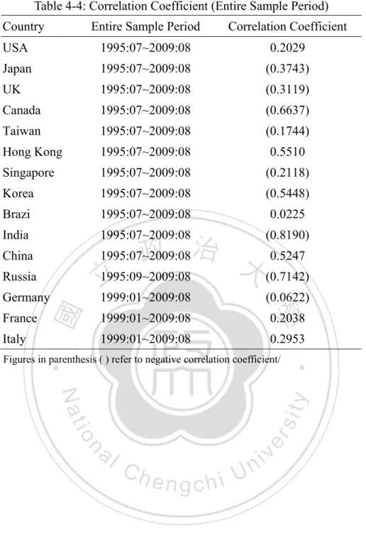
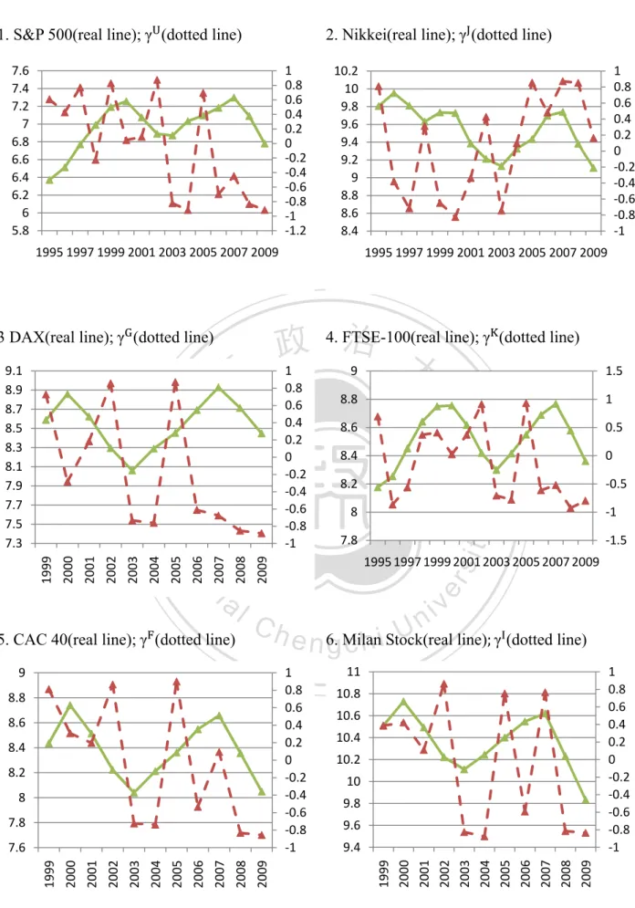
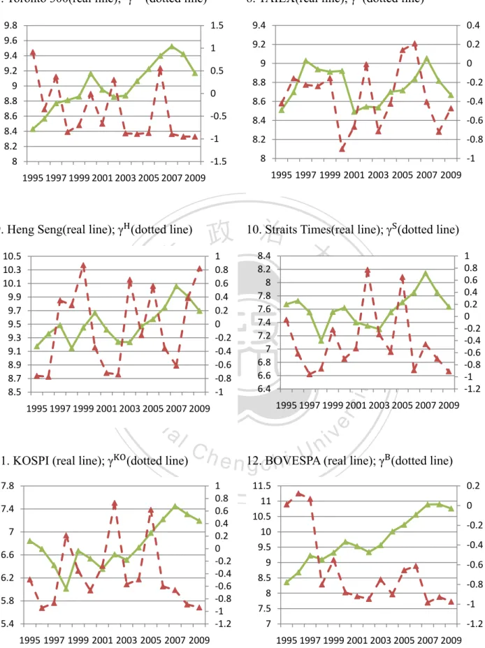
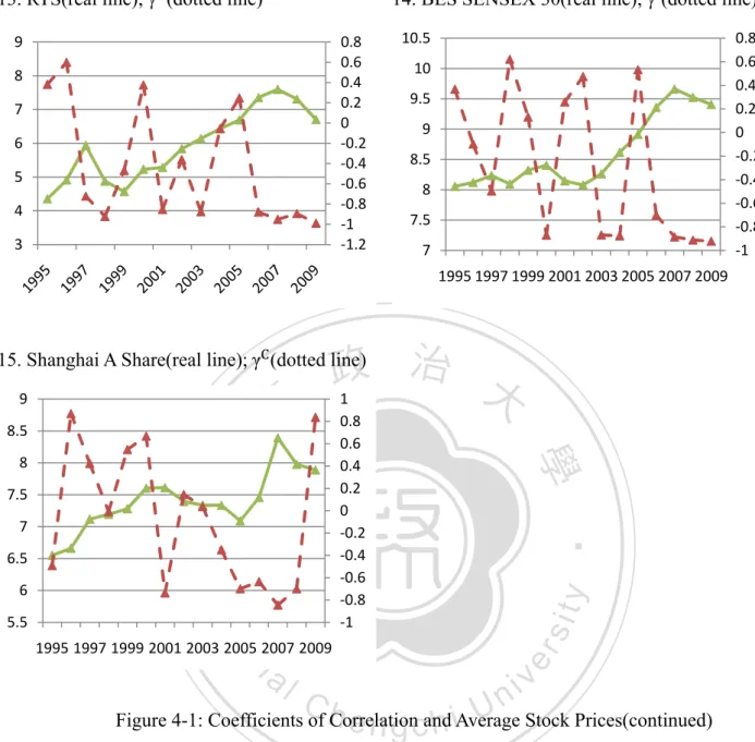
(30) . beginning in 2007 to 2009. That is, the stock markets plunge while the currencies depreciate. More tendencies can be observed if the entire 15-year sample period is taken into consideration. Before 2000, the global tendency in the relationship between exchange rates and stock markets is not clear. Nevertheless, since 2000, the integration of global tendency has been more observable and convincing. This is mainly thanks to financial globalization resulting from the freer worldwide trade and electronic trading system after the Millennium. Moreover, we can notice another long-term trend from table 4-4.. 政治大 developed countries and emerging countries are not conclusive. 5 countries including 立. Results shown in table 4-4 indicate that the coefficients of correlation between. France, Italy, Hong Kong, Brazil and China have shown positive coefficients of. ‧ 國. 學. correlation, while the other nine countries—USA, Japan, Germany, UK, Canada,. ‧. Taiwan, Singapore, Korean, Russia and India, have shown negative.. y. Nat. Lastly, we draw the attention back to table 4-3 and figure 4-1. Since the. er. io. sit. beginning of a bull market in 2002, the coefficients of correlation between stock markets and exchange rates in these countries have become stronger. The frequency of. al. n. v i n negative correlation coefficientsCsmaller than minus 5U h e n g c h i in 2002 is 2. Afterwards, it has increased from 12 countries in 2003 to 13 in 2008 and 11 in 2009. The numbers are. closely in accordance with that of negative coefficients. This implies a highly powerful relationship between the two variables. We also can discern the volatility of correlation coefficients for each country from figure 4-1. The vigorous fluctuations occur in almost every country except Brazil. In other words, the coefficients’ great volatility and the same direction of their fluctuations across countries reveal another evidence of worldwide integration in financial markets.. 24 .

(31) . Table 4-3: Correlation Coefficients of Stock Prices and Exchange Rates (Annually) 1995. 1996. 1997. 1998. 1999. 2000. 2001. 2002. USA. 0.8145. 0.0804. 0.6066. (0.7302) (0.0957) (0.3580) (0.3731) 0.8082. Japan. 0.8106. (0.3801) (0.7165) 0.3122. 2003. 2004. 2005. 2006. 2007. 2008. 2009. No. of ( ). γ < -0.5. (0.9362) (0.8031) 0.7628. (0.5921) (0.5543) (0.9445) (0.9219). 10. 7. (0.6495) (0.8249) (0.3368) 0.4273. (0.7443) 0.0975. 0.4814. 6. 4. 0.7277. (0.2838) 0.1835. 0.8565. (0.7335) (0.7616) 0.8710. (0.6113) (0.6766) (0.8522) (0.8826). 7. 6. 0.4102. 0.0254. 0.3703. 0.9134. France. 0.8110. 0.3078. Italy. 0.3867. 0.4225. UK. 0.6943. (0.8665) (0.5623) 0.3698. 0.8524. 0.1640. (0.6125) (0.5198) (0.9264) (0.7978). 8. 8. 0.1976. (0.5342) 0.0941. (0.8310) (0.8559). 5. 5. 0.1103. 0.8647. (0.5925) 0.7664. (0.8147) (0.8350). 5. 5. (0.8938) (0.9498) (0.9488). 11. 9. (0.4053) (0.7198) (0.4722). 13. 4. 8. 5. (0.8472) (0.6974) (0.0069) (0.6652) 0.3022. (0.8263) (0.8752) 0.7525. 學. 0.9148. Taiwan. (0.4212) (0.1570) (0.2252) (0.2400) (0.1554) (0.8999) (0.6671) (0.0092) (0.7142) (0.4242) 0.1406. 0.2098. HK. (0.7611) (0.7738) 0.3511. (0.3532) (0.6104) 0.3844. Singapore. (0.0544) (0.6150) (0.9561) (0.8644) (0.2193) (0.7020) (0.5283) 0.7722. (0.2942) (0.5872) 0.6536. (0.8891) (0.4592) (0.6987) (0.9075). 13. 9. Korea. (0.4917) (0.9462) (0.8658) 0.2120. (0.5689) (0.4899) 0.6206. (0.6012) (0.6601) (0.8911) (0.9384). 12. 8. Brazil. 0.0115. 0.1232. 0.0676. (0.8000) (0.5508) (0.8804) (0.9189) (0.9461) (0.7493) (0.9001) (0.6553) (0.6118) (0.9832) (0.9262) (0.9746). 12. 12. Russia. 0.3818. 0.5999. (0.7207) (0.9221) (0.4691) 0.3758. (0.8782) (0.9507) (0.8944) (0.9882). 11. 8. India. 0.3672. (0.0982) (0.4957) 0.6208. (0.6992) (0.8853) (0.9118) (0.9218). 9. 7. China. (0.4914) 0.8694. 0.4234. (0.0089) 0.5474. 0.6677. (0.7366) 0.1456. 0.0366. (0.3504) (0.6993) (0.6357) (0.8455) (0.6992) 0.8366. 8. 5. No. of ( ). 5. 8. 7. 7. 8. 10. 10. 4. 13. 14. 3. 12. 12. 13. 12. 138. γ < -0.5. 1. 4. 5. 5. 3. 6. 7. 2. 12. 9. 3. 11. 10. 13. 11. 102. (0.3415) (0.7175) (0.7403) 0.6553. Nat. io. (0.3531) (0.6672) (0.2748) 0.7310. n. al. 0.1314. Ch. engchi. i n U. (0.8704) 0.2587. 0.4746. (0.8685) (0.8758) 0.5328. 25 . 0.8219. v. (0.8530) (0.3607) (0.8755) (0.0545) 0.2482. Figures in parenthesis ( ) refer to negative correlation coefficient.. . (0.1607) 0.5626. y. 0.8702. sit. 0.2799. (0.8781) (0.8906) (0.8705) 0.5594. ‧. Canada. er. (0.3474) 0.3718. 0.8723. 治 (0.7797) 0.9323 政 (0.7070) 大 0.8649 (0.7246) (0.7378) 0.8998. 立. ‧ 國. Germany. 0.8556. 102.

(32) . Table 4-4: Correlation Coefficient (Entire Sample Period) Entire Sample Period. Correlation Coefficient. USA. 1995:07~2009:08. 0.2029. Japan. 1995:07~2009:08. (0.3743). UK. 1995:07~2009:08. (0.3119). Canada. 1995:07~2009:08. (0.6637). Taiwan. 1995:07~2009:08. (0.1744). Hong Kong. 1995:07~2009:08. 0.5510. Singapore. 1995:07~2009:08. (0.2118). Korea. 1995:07~2009:08. (0.5448). Brazi. 1995:07~2009:08. 0.0225. India. 1995:07~2009:08. (0.8190). 1999:01~2009:08. (0.0622). 1999:01~2009:08. 學. Country. 1999:01~2009:08. 0.2953. 政治大 0.5247 1995:07~2009:08 1995:09~2009:08 (0.7142) 立. China Russia France Italy. 0.2038. Figures in parenthesis ( ) refer to negative correlation coefficient/. n. er. io. sit. y. Nat. al. Ch. engchi. 26 . ‧. ‧ 國. Germany. i n U. v.

(33) . 1. S&P 500(real line); γU (dotted line). 2. Nikkei(real line); γJ (dotted line) 1 0.8 0.6 0.4 0.2 0 ‐0.2 ‐0.4 ‐0.6 ‐0.8 ‐1 ‐1.2. 7.6 7.4 7.2 7 6.8 6.6 6.4 6.2 6 5.8 1995 1997 1999 2001 2003 2005 2007 2009. K. 8.4. 8 7.8. 8.2 8 7.8. v. 11. 1 0.8 0.6 0.4 0.2 0 ‐0.2 ‐0.4 ‐0.6 ‐0.8 ‐1. 10.8 10.6 10.4 10.2 10 9.8 9.6 9.4. Figure 4-1: Coefficients of Correlation and Average Stock Prices 27 . ‐1. er. i n U. 2009. 2008. 2007. 2006. 2005. 2004. 2003. 2002. 2001. 2000. 1999. 7.6. ‐1.5. 1999 2000 2001 2002 2003 2004 2005 2006 2007 2008 2009. 8.4. ‐0.5. y. 8.2. n. 8.6. 0. e n 6.gMilan c h iStock(real line); γI(dotted line). 1 0.8 0.6 0.4 0.2 0 ‐0.2 ‐0.4 ‐0.6 ‐0.8 ‐1. 8.8. 0.5. 1995 1997 1999 2001 2003 2005 2007 2009. Ch. 9. 1. 8.6. 2009. 2008. 2007. 2006. 2005. 2004. 2003. 2002. 2001. 2000. io. 5. CAC 40(real line); γF (dotted line). 1.5. ‧. Nat. al. 8.8. 學. ‧ 國. 0.8 0.6 0.4 0.2 0 ‐0.2 ‐0.4 ‐0.6 ‐0.8 ‐1. sit. 立. 1999. 1995 1997 1999 2001 2003 2005 2007 2009. FTSE-100(real line); γ (dotted line) 政 4. 治大 1 9. 3 DAX(real line); γG (dotted line) 9.1 8.9 8.7 8.5 8.3 8.1 7.9 7.7 7.5 7.3. 1 0.8 0.6 0.4 0.2 0 ‐0.2 ‐0.4 ‐0.6 ‐0.8 ‐1. 10.2 10 9.8 9.6 9.4 9.2 9 8.8 8.6 8.4.

(34) . 8. TAIEX(real line); γT (dotted line). 7. Toronto 300(real line); γCA (dotted line) 9.8 9.6 9.4 9.2 9 8.8 8.6 8.4 8.2 8. 1.5. 9.4. 0.4. 1. 9.2. 0.2. 8.8. ‐0.2. 8.6. ‐0.4. ‐0.5. 8.4. ‐0.6. ‐1. 8.2. ‐0.8. 0. 1995 1997 1999 2001 2003 2005 2007 2009. 1995 1997 1999 2001 2003 2005 2007 2009. Straits Times(real line); γ (dotted line) 政 10.治大 8.4 1 1 S. er. n. 7 6.6 6.2 5.8 5.4. i n U. v. (real line); γB (dotted line) e n 12. hi g cBOVESPA. 1 0.8 0.6 0.4 0.2 0 ‐0.2 ‐0.4 ‐0.6 ‐0.8 ‐1 ‐1.2. 7.4. y. ‧ 國 io. Ch. 7.8. ‧. Nat. 11. KOSPI (real line); γKO (dotted line). 0.2. 11.5 11 10.5 10 9.5 9 8.5 8 7.5 7. 1995 1997 1999 2001 2003 2005 2007 2009. 0 ‐0.2 ‐0.4 ‐0.6 ‐0.8 ‐1 ‐1.2 1995 1997 1999 2001 2003 2005 2007 2009. Figure 4-1: Coefficients of Correlation and Average Stock Prices(continued) 28 . 0.8 0.6 0.4 0.2 0 ‐0.2 ‐0.4 ‐0.6 ‐0.8 ‐1 ‐1.2. 1995 1997 1999 2001 2003 2005 2007 2009. 1995 1997 1999 2001 2003 2005 2007 2009. al. 學. 8.2 8 7.8 7.6 7.4 7.2 7 6.8 6.6 6.4. 0.8 0.6 0.4 0.2 0 ‐0.2 ‐0.4 ‐0.6 ‐0.8 ‐1. sit. 立. 10.5 10.3 10.1 9.9 9.7 9.5 9.3 9.1 8.9 8.7 8.5. ‐1. 8. ‐1.5. 9. Heng Seng(real line); γH (dotted line). 0. 9. 0.5.

(35) . 13. RTS(real line); γR (dotted line). 14. BES SENSEX 30(real line); γI (dotted line). 9. 0.8 0.6 0.4 0.2 0 ‐0.2 ‐0.4 ‐0.6 ‐0.8 ‐1 ‐1.2. 8 7 6 5 4 3. 0.8 0.6 0.4 0.2 0 ‐0.2 ‐0.4 ‐0.6 ‐0.8 ‐1. 10.5 10 9.5 9 8.5 8 7.5 7 1995 1997 1999 2001 2003 2005 2007 2009. 政治大 1. 15. Shanghai A Share(real line); γC (dotted line). 7.5. 6.5. Nat. 6 5.5. ‧. 7. y. 8. 學. 0.8 0.6 0.4 0.2 0 ‐0.2 ‐0.4 ‐0.6 ‐0.8 ‐1. ‧ 國. 8.5. io. sit. 立. 9. n. al. er. 1995 1997 1999 2001 2003 2005 2007 2009. Ch. engchi. i n U. v. Figure 4-1: Coefficients of Correlation and Average Stock Prices(continued). 29 .

(36) . 4.3 Johansen cointegration test Since the series are of the same order, i.e., Ι (1), as we have tested in the unit-root test, we proceed to test the existence of cointegrating relations among the stock prices and exchange rates using the Johansen cointegration test. The lag length is chosen by applying the Akaike Info Criterion (AIC) on the unrestricted VAR. Between Johansen’s two likelihood ratio tests for cointegration, the trace test shows more robustness to both skewness and kurtosis (i.e., normality) in residuals than the maximum eigenvalue test4. Thus, we employ only the trace test to perform the. 政治大 The results are reported in table 4-5. As can be seen in the table, for G-7 and 立. cointegration test... some emerging countries, except Russia and China, the null hypothesis of no. ‧ 國. 學. cointegration cannot be rejected using a 5 percent significance level. Analyzed. ‧. financial markets in all developed countries do not share the same stochastic trend and. y. Nat. consequently no stable long-term linkages between the variable exist. However, the. relationship between stock prices and exchange rates.. al. v i n C hequilibrium relationship long-run engchi U. n. Our findings of no. er. io. sit. results for emerging markets are mixed. Both Russia and China demonstrate stronger. between two financial. variables are in contrast with Ajayi and Mougoué (1996), but mostly consistent with those of Bahmani-Oskooee and Sohrabian (1992) and Baharom, Habibullah and Royfaizal (2008)..                                                        . 4. See Cheung and Lai (1993) for details. 30 . .

(37) . Table 4-5: Johansen Cointegration Test (Trace Test Statistics) Country. HO. H. Eigenvalue. Statistic. USA 1995:07~2009:8. ρ=o. ρ≥0. 0.0483. 9.4183. ρ=1. ρ≥1. 0.0069. 1.1520. ρ=o. ρ≥0. 0.0478. 12.5875. ρ=1. ρ≥1. 0.0256. 4.3614. ρ=o. ρ≥0. 0.0334. 6.5206. ρ=1. ρ≥1. 0.0175. 2.2282. ρ=o. ρ≥0. 0.0356. 10.2000. ρ=1. ρ≥1. 0.0244. 4.1333. 政 ρ≥1 治大0.0123. 6.2350. Japan 1995:07~2009:8 Germany 1999:01~2009:8 United Kingdom 1995:07~2009:8 France 1999:01~2009:8. ρ=o. ρ≥0. ρ=1 Italy. 1995:07~2009:8. ρ=1. ρ≥1. 0.0097. 1.2307. ρ=o. ρ≥0. 0.0551. 10.4060. ρ=1. ρ≥1. 0.0056. 0.9402. ρ=o. ρ≥0. 0.0564. ρ=1. ρ≥1. 0.0260. ρ≥0. 0.0625. ρ=o. n. al. y. sit. i n U. v. 4.4229 14.5883. 0.0226. 3.8126. 0.0621. 15.2738. ρ≥1. 0.0264. 4.4998. ρ=o. ρ≥0. 0.0600. 12.1133. ρ=1. ρ≥1. 0.0110. 1.8305. ρ=o. ρ≥0. 0.0564. 12.0566. ρ=1. ρ≥1. 0.0140. 2.3567. ρ=o. ρ≥0. 0.1104. 22.8223*. ρ=1. ρ≥1. 0.0212. 3.5283. ρ=o. ρ≥0. 0.0386. 8.4636. ρ=1. ρ≥1. 0.0112. 1.8823. ρ=o. ρ≥0. 0.1758. 35.2353*. ρ=1. ρ≥1. 0.0187. 3.1334. ρ=1 Singapore 1995:07~2009:8. 14.1734. er. Hong Kong. 6.0308. Nat. 1995:07~2009:8. 0.0374. ‧. Taiwan. ρ≥0. ‧ 國. 1995:07~2009:8. 立. 學. Canada. ρ=o. 1.5598. io. 1999:01~2009:8. 0.0364. ρ=o ρ=1. Ch. ρ≥1. e nρ≥0g c h i. Korea 1995:07~2009:8 Brazil 1995:07~2009:8 Russia 1995:09~2009:8 India 1995:07~2009:8 China 1995:07~2009:8. * denotes the rejection of null hypothesis at 5% significance level. 31 .

(38) . 5. Conclusions In this study, we examine the correlation and cointegration between stock markets and exchange markets for G-7 and 8 emerging countries, including USA, Japan, Germany, UK, France, Italy, Canada, Taiwan, Hong Kong, Singapore, Korea, Brazil, Russia, India and China. Our empirical results show a significant correlation between. the. two. said. variables. chronologically,. especially. after. 2000.. Geographically, emerging countries tend to possess negative correlations but the results in this study are mixed. Yet, we can observe an obvious regional tendency, for. 政治大. instance, in the European countries and among Asian’s trade-led countries such as. 立. Taiwan, Singapore and Korea. These countries in the same region and have the same. ‧ 國. 學. pattern of trade tend to share common trend of correlations. Further, our findings of Johansen cointegration test for these 15 countries are also consistent. Cointegration of. Nat. y. ‧. stock prices and exchange rates does not exist in 13 countries.. sit. There has been an overall co-movement for the world since the beginning of this. n. al. er. io. century. This paper postulates that the contrast in the findings between the advanced. i n U. v. and emerging countries put forward by earlier literature are due to the differences in. Ch. engchi. the structure and characteristics of financial markets between the groups before 2000. As the level of integration in the worldwide financial markets as well as the rapid development of electronic trading system, it is inevitable that even a local problem could be contagious and may affect the whole world. We believe this is the reason why the Greece’s economic crisis has great impact on the world economy and should be dealt with immediately and properly.. 32 .

(39) . References Abdalla, I. S. A. and V. Murinde, 1997, “Exchange Rate and Stock Price Interactions in Emerging Financial Markets: Evidence on India, Korea, Pakistan, and Philippines.” Applied Financial Economics 7, 25–35. Aggarwal, R., 1981, “Exchange Rates and Stock Prices: A Study of U.S. Capital Market under Floating Exchange Rates,” Akron Business and Economic Review, 7–12. Ajayi, R. A. and M. Mougoue. 1996, “On the Dynamic Relation between. 政治大 Baharom, A.H. and M.S. Habibullah 立 and R.C., Royfaizal, 2008, "Pre and Post Crisis. Stock Prices and Exchange Rates,” Journal of Financial Research 19, 193–207.. ‧ 國. Paper 12445, University Library of Munich, Germany.. 學. Analysis of Stock Price and Exchange Rate: Evidence from Malaysia," MPRA. ‧. Bahmani-Oskooee, M. and A. Sohrabian, 1992, “Stock Prices and the Effective. sit. y. Nat. Exchange Rate of the Dollar,” Applied Economics 24, 459–464.. al. er. io. Bartov, E. and G. M. Bodnar, 1994, “Firm Valuation, Earnings Expectations, and. v. n. The Exchange-Rate Exposure Effect,” Journal of Finance 49, 1755–1785.. Ch. engchi. i n U. Branson, W. H., 1983, “Macroeconomic Determinants of Real Exchange Risk,” in Managing Foreign Exchange Risk, R. J. Herring ed., Cambridge: Cambridge University Press Cheung, Y. W. and K. S. Lai., 1993, “Finite Sample Sizes of Johansen’s Likelihood Ratio Tests for Cointegration,” Oxford Bulletin of Economics and Statistics 55: 3, 313–328. Donnelly, R. and E. Sheehy, 1996, “The share price reaction of U.K. exporters to exchange rate movements: An empirical study,” Journal of International Business Studies 27, 157−165. 33 .

(40) . Dornbusch, R. and S. Fisher, 1980, "Exchange Rates and the Current Account," American Economic Review 70, 960-971. Franck, P. and A. Young, 1972, “Stock Price Reaction of Multinational Firms to Exchange Realignments,” Financial Management 1, 1972, 66–73. Frankel, J.A., 1983, "Monetary and Portfolio Balance Models of Exchange Rate Determination", in J.S. Bhandari and B. H. Putnam (eds) "Economic Interdependence and Flexible Exchange Rates," MIT Press, Cambridge, MA. Granger, C.W.J. and I. Newbold, 1974, “Spurious regressions in econometrics,”. 政治大 Johansen, S., 1991, “Estimation and Hypothesis Testing of Cointegrating Vectors in 立 Journal of Econometrics 2, 111-120.. Gaussian Vector Autoregressive Models,” Econometrica 59: (November), 1551–. ‧ 國. 學. 1580.. ‧. Johansen, S. and K. Juselius, 1990, “Maximum Likelihood Estimation and Inference. y. Nat. on Cointegration with Application to the Demand for Money,” Oxford Bulletin of. er. io. sit. Economics and Statistics 52, 169–210.. Ma, C. K. and G. W. Kao, 1990, “On Exchange Rate Changes and Stock Price. al. n. v i n C h Finance and Accounting, Reactions,” Journal of Business 17(3), 441-450. engchi U. Muhammad, N. and A. Rasheed, 2003, “Stock Prices and Exchange Rates: Are they Related? Evidence from South Asian Countries”, Paper presented at the 18th Annual General Meeting and Conference of the Pakistan Society of Development Economists, January 2003. Pan, M.S., R.C.W. Fok and Y.A. Liu, 2007, “Dynamic Linkages between Exchange Rates and Stock Prices: Evidence from East Asian Markets”, International Review of Economics and Finance 16, 2007, 503-520. Phylakits, K. and Ravazzolo, F., 2000, “Stock Prices and Exchange Rate Dynamics,” Paper presented at the EFMA 2000 Meeting in Athens, May 2000. 34 .

(41) . Rittenberg, L., 1993, “Exchange Rate Policy and Price Level Changes: Causality Tests for Turkey in the Post-Liberalisation Period”, the Journal of Development Studies 29:2, 321–332. Smith, C., 1992, “Stock Market and the Exchange Rate: A Multi-Country Approach,” Journal of Macroeconomics 14, 607–629. Soenen, L.A. and E.S. Hennigar, 1988, "An Analysis of Exchange Rates and Stock Prices - The US Experience between 1980 and 1986," Akron Business and Economic Review:(Winter), 7-16.. 政治大 Journal of Finance, 42(1), 141-149. 立. Solnik, B., 1987, “Using Financial Prices to Test Exchange Rate Models: A Note,”. Stavarek, D., 2004, “Stock Prices and Exchange Rates in the EU and the USA:. ‧ 國. 學. Evidence of their Mutual Interactions,” MPRA Paper 7297, University Library of. ‧. Munich, Germany.. y. Nat. Yang, S.Y. and S.C. Doong, 2004, “Price and Volatility Spillovers between Stock. er. io. sit. Prices and Exchange Rates: Empirical Evidence from the G-7 Countries,” International Journal of Business and Economics 3, 2004, 139-153.. al. n. v i n CExchange Yu, Q., 1997, “Stock Prices and Experience in Leading East Asian U h e n gRates: i h c Financial Centres: Tokyo, Hong Kong and Singapore”, Singapore Economic Review 41, 47–56. Wu, Y., 2000, “Stock Prices and Exchange Rates in a VEC Model—the Case of Singapore in the 1990s,” Journal of Economics and Finance 24, 260-274.. 35 .

(42)